The Poisson binomial distribution – Old & New
Abstract.
This is an expository article on the Poisson binomial distribution. We review lesser known results and recent progress on this topic, including geometry of polynomials and distribution learning. We also provide examples to illustrate the use of the Poisson binomial machinery. Some open questions of approximating rational fractions of the Poisson binomial are presented.
Key words : Distribution learning, geometry of polynomials, Poisson binomial distribution, Poisson/normal approximation, optimal transport, stochastic ordering, strongly Rayleigh property.
1. Introduction
The binomial distribution is one of the earliest examples a college student encounters in his/her first course in probability. It is a discrete probability distribution of a sum of independent and identically distributed (i.i.d.) Bernoulli random variables, modeling the number of occurrence of some events in repeated trials. An integer-valued random variable is called binomial with parameters , denoted as , if , . It is well known that if is large, the distribution is approximated by the Poisson distribution for small ’s, and is approximated by the normal distribution for larger values of . See e.g. [77] for an educational tour.
Poisson [81] considered a more general model of independent trials, which allows heterogeneity among these trials. Precisely, an integer-valued random variable is called Poisson binomial, and denoted as if
where are independent Bernoulli random variables with parameters . It is easily seen that the probability distribution of is
| (1.1) |
where the sum ranges over all subset of of size .
The Poisson binomial distribution has a variety of applications such as reliability analysis [16, 57], survey sampling [29, 104], finance [40, 92], and engineering [44, 100]. Though this topic has been studied for a long time, the literature is scattered. For instance, the Poisson binomial distribution has different names in various contexts: Pólya frequency (PF) distribution, strongly Rayleigh distribution, convolutions of heterogenous Bernoulli, etc. Researchers often work on some aspects of this subject, and ignore its connections to other fields. In late 90’s, Pitman [78] wrote a survey on the Poisson binomial distribution with focus on probabilizing combinatorial sequences. Due to its applications in modern technology (e.g. machine learning [25, 89], causal inference (Example 3.4)) and links to different mathematical fields (e.g. algebraic geometry, mathematical physics), we are motivated to survey recent studies on the Poisson binomial distribution. While most results in this paper are known in some form, several pieces are new (e.g. Section 4). The aim of this paper is to provide a guide to lesser known results and recent progress of the Poisson binomial distribution, mostly post 2000.
The rest of the paper is organized as follows. In Section 2, we review distributional properties of the Poisson binomial distribution. In Section 3, various approximations of the Poisson binomial distribution are presented. Section 4 is concerned with the Poisson binomial distribution and polynomials with nonnegative coefficients. There we discuss the problem of approximating rational fractions of Poisson binomial. Finally in Section 5, we consider some computational problems related to the Poisson binomial distribution.
2. Distributional properties of Poisson binomial variables
In this section, we review a few distributional properties of the Poisson binomial distribution. For , we have
| (2.1) |
where . It is easily seen that by keeping (or ) fixed, the variance of is increasing as the set of probabilities gets more homogeneous, and is maximized as . There is a simple interpretation in survey sampling: taking samples from different communities (stratified sampling) is better than taking from the same group (simple random sampling).
The above observation motivates the study of stochastic orderings for the Poisson binomial distribution. The first result of this kind is due to Hoeffding [53], claiming that among all Poisson binomial distributions with a given mean, the binomial distribution is the most spread-out.
Theorem 2.1.
[53] (Hoeffding’s inequalities) Let , and .
- (1)
There are inequalities
and
- (2)
For any convex function in the sense that , , we have
where the equality holds if and only if .
The part (2) in Theorem 2.1 indicates that among all Poisson binomial distributions, the binomial is the largest one in convex order. This result was extended to the multidimensional setting [9], and to non-negative random variables [8, Proposition 3.2]. See also [68] for interpretations. Next we give several applications of Hoeffding’s inequalities.
Examples 2.2.
- (1)
Monotonicity of binomials. Fix . By taking , we get for and ,
Similarly, by taking , we get for and ,
These inequalities were used in [3] to derive the monotonicity of error in approximating the binomial distribution by a Poisson distribution. By letting and , they proved is positive if and is negative if . The result quantifies the error of confidence levels in hypothesis testing when approximating the binomial distribution by a Poisson distribution.
- (2)
Darroch’s rule. It is well known that a Poisson binomial variable has either one, or two consecutive modes. By an argument in the proof of Hoeffding’s inequalities, Darroch [32, Theorem 4] showed that the mode of the Poisson binomial distribution differs from its mean by at most . Precisely, he proved that
(2.2) This result was reproved in [91]. See also [60] for a similar result concerning the median.
- (3)
Azuma-Hoeffding inequality. By the Azuma-Hoeffding inequality [5, 54], for independent random variables such that ,
(2.3) where . Now we show how to derive a version of (2.3) via a Poisson binomial trick. Given , let be independent Bernoulli with parameter and . We have
(2.4) Given , is Poisson binomial with mean greater than . According to Hoeffding’s inequality,
(2.5) for some universal constant . Combining (2.4) and (2.5) yields . Note that is Poisson binomial with mean . Applying Hoeffding’s inequality to with bounds for binomial tails [71], we get
(2.6) As a consequence, which achieves the same rate as in (2.3) up to a constant factor.
The original proof of Theorem 2.1 was brute-force, and it was soon generalized by using the idea of majorization and Schur convexity. To proceed further, we need some vocabularies. Let be the order statistics of .
Definition 2.3.
The vector is said to majorize the vector , denoted as , if
See [66] for background and development on the theory of majorization and its applications. The following theorem gives a few lesser known variants of Hoeffding’s inequalities.
Theorem 2.4.
The proof of Theorem 2.4 relies on the fact that implies the components of are more spread-out than those of . For example in part (1), it boils down to proving if , is a Schur concave function in , meaning its value increases as the components of are less dispersed. The part (3) gives a sufficient condition of stochastic orderings for the Poisson binomial distribution. A simple necessary and sufficient condition remains open. See also [15, 16, 18, 52, 93, 107] for further results.
3. Approximation of Poisson binomial distributions
In this section, we discuss various approximations of the Poisson binomial distribution. Pitman [78, Section 2] gave an excellent survey on this topic in the mid-90’s. We complement the discussion with recent developments. In the sequel, denotes the distribution of a random variable .
Poisson approximation. Le Cam [64] gave the first error bound for Poisson approximation of the Poisson binomial distribution. The following theorem is an improvement of Le Cam’s bound.
Theorem 3.1.
It is easily seen from (3.1) that the Poisson approximation of the Poisson binomial is good if , or equivalently . There are two cases:
- •
For small , the upper bound in (3.1) is sharp.
- •
For large , the approximation error is of order .
As pointed out in [59], the constant in the lower bound can be improved to . See [6] for a book-length treatment, and [86] for sharp bounds. A powerful tool to study the approximation of the sum of (possibly dependent) random variables is Stein’s method of exchangeable pairs, see [26]. For instance, a simple proof of the upper bound in (3.1) was given in [26, Section 3] via the Stein machinery.
The Poisson approximation can be viewed as a mean-matching procedure. The failure of the Poisson approximation is due to a lack of control in variance. A typical example is where all ’s are bounded away from , so that is large and is of constant order. To deal with these cases, Röllin [85] proposed a mean/variance-matching procedure. To present further results, we need the following definition.
Definition 3.2.
An integer-valued random variable is said to be translated Poisson distributed with parameters , denoted as , if , where is the fraction part of a positive number.
It is easy to see that a random variable has mean , and variance which is between and . The following theorem gives an upper bound in total variation between a Poisson binomial variable and its translated Poisson approximation.
Theorem 3.3.
Note that if all ’s are bounded away from and , the approximation error is of order which is optimal. See [70] for the most up-to-date results of the Poisson approximation. Now we give an application of translated Poisson approximation in observational studies.
Example 3.4.
Sensitivity analysis. In matched-pair observational studies, an sensitivity analysis accesses the sensitivity of results to hidden bias. Here we follow a modern approach of Rosenbaum [88, Chapter 4]. Precisely, the sample consists of matched pairs and units in each pair are indexed by . Each pair is matched on a set of observed covariates , and only one unit in each pair receives the treatment. Let be the treatment assignment, so . Common test statistics for matched pairs are sign-score statistics of the form: , where and . For simplicity, we take and the statistics of interest are
| (3.3) |
where is Bernoulli distributed with parameter with . So . For , let , which equals to if there is no hidden bias.
The goal is to make inference on with different choices of and understand which choices explain away the conclusion we draw from the null hypothesis (i.e. there is no hidden bias). Thus, we are interested in the set
on the boundary of which the conclusion assuming no hidden bias is turned over. However, direct computation of seems hard. A routine way to solve this problem is to approximate by a regular shape. To this end, we consider the following optimization problem:
| (3.4) |
where is a constraint region. For instance, corresponds to the worst-case sensitivity analysis. By the translated Poisson approximation, the quantity can be evaluated by the following problem which is easy to solve.
| (3.5) |
Normal approximation. The normal approximation of the Poisson binomial distribution follows from Lyapunov or Lindeberg central limit theorem, see e.g. [11, Section 27]. Berry and Esseen independently discovered an error bound in terms of the cumulative distribution function for the normal approximation of the sum of independent random variables. Subsequent improvements were obtained by [72, 75, 94, 102] via Fourier analysis, and by [27, 28, 67, 101] via Stein’s method.
Let be the probability density function of the standard normal, and be its cumulative distribution function. The following theroem provides uniform bounds for the normal approximation of Poisson binomial variables.
Theorem 3.5.
Other than uniform bounds (3.6)-(3.7), several authors [14, 49, 84] studied error bounds for the normal approximation in other metrics. For , two probability measures, consider
- •
metric
- •
Wasserstein’s metric
where the infimum runs over all probability measures on with marginals and .
Specializing these bounds to the Poisson binomial distribution, we get the following result.
Theorem 3.6.
Goldstein [49] proved bound (3.8) for with . The general case follows from the inequality together with Goldstein’s bound and the uniform bound (3.7). By the Kantorovich-Rubinstein duality, . So the bound (3.9) holds for with . For general , the bound (3.9) is a consequence of the fact that for with ’s independent, and ,
This result was proved in [84] for , and generalized to all in [14].
Binomial approximation. The binomial approximation of the Poisson binomial is lesser known. The first result of this kind is due to Ehm [41] who proved that for ,
| (3.10) |
Elm’s approach was extended to a Krawtchouk expansion in [87]. The advantage of the binomial approximation over the Poisson approximation is justified by the following result due to Choi and Xia [31].
Theorem 3.7.
Let , and . For , let . Then for sufficiently large,
| (3.11) |
4. Poisson binomial distributions, polynomials with nonnegative coefficients and optimal transport
In this section, we discuss aspects of the Poisson binomial distribution related to polynomials with nonnegative coefficients. For , the probability generating function (PGF) of is
| (4.1) |
It is easy to see that is a polynomial with all nonnegative coefficients, and all of its roots are real negative. The story starts with the following remarkable theorem, due to Aissen, Endrei, Schoenberg and Whitney [1, 2].
Theorem 4.1.
[1, 2] Let be a sequence of nonnegative real numbers, with associated generating polynomial . The following conditions are equivalent:
- (1)
The polynomial has only real roots.
- (2)
The sequence is the probability distribution of a distribution for some . The real roots of are for with .
- (3)
The sequence is a Pólya frequency (PF) sequence, i.e. the Toeplitz matrix is totally nonnegative.
See [4] for background on total positivity. From a computational aspect, the condition (3) amounts to solving a system of polynomial inequalities [42, 46]. Theorem 4.1 justifies the alternative name ‘PF distribution’ for the Poisson binomial distribution. Standard references for PF sequences are [22, 96]. See also [78] for probabilistic interpretations for polynomials with only negative real roots, and [55] for various extensions of Theorem 4.1 by linear algebra.
A polynomial is called stable if it has no roots with positive imaginary part, and a stable polynomial with all real coefficients is called real stable [19, 20]. In [21], a discrete distribution is said to be strongly Rayleigh if its PGF is real stable. It was also shown that the strong Rayleigh property enjoys all virtues of negative dependence. The following result is a simple consequence of Theorem 4.1.
Corollary 4.2.
A random variable for some if and only if is strongly Rayleigh on .
In the sequel, we use the terminologies ‘Poisson binomial’ and ‘strongly Rayleigh’ interchangeably. Call a polynomial with strongly Rayleigh if it satisfies one of the conditions in Theorem 4.1.
For , it is hopeless to get any ‘simple’ necessary and sufficient condition for to be strongly Rayleigh due to Abel’s impossibility theorem. A necessary condition for to be strong Rayleigh is the Newton’s inequality:
| (4.2) |
The sequence satisfying (4.2) is also said to be ultra-logconcave [74]. Consequently, is logconcave and unimodal. A lesser known sufficient condition is given in [58, 63]:
| (4.3) |
See also [50, 61] for various generalizations. As observed in [62], the inequality (4.3) cannot be improved since the sequence defined by decreases from to its limit approximately .
In recent work [47], the authors considered the multivariate CLT from strongly Rayleigh property. They raised the following question: if is a strong Rayleigh, or Poisson binomial random variable, how well can one approximate for each by a strong Rayleigh, or Poisson binomial random variable ? A good approximation combined with the Crámer-Wold device proves the CLT for multivariate strongly Rayleigh variables. The case was solved in that paper.
Theorem 4.3.
[47] Let be a strongly Rayleigh random variable. Then is strongly Rayleigh for each , where is the integer part of .
The key to the proof of Theorem 4.3 is [47, Theorem 4.3]: For a polynomial of degree and , write , with a polynomial of degree . The theorem asserts that if is strongly Rayleigh, then so are ’s with interlacing roots. In fact, the real-rootedness follows from the fact that
for each and . This result is well known, see [1, Theorem 7] or [22, Theorem 3.5.4]. But the root interlacing seems less obvious by Pólya frequency sequences.
A natural question is whether is strongly Rayleigh for each . It turns out that can be far away from being strongly Rayleigh. In fact, one can prove the following theorem.
Theorem 4.4.
Let , and be the roots of the probability generating function of . Then
| (4.4) |
where is the imaginary part of .
The reason why some roots of the PGF of have large positive imaginary parts is due to the unbalanced allocation of probability weights to even and odd numbers: while . So the Newton’s inequality (4.2) is not satisfied.
Optimal transport. For simplicity, we consider . The goal is to find a coupling which is strongly Rayleigh on such that is as small as possible. Now we provide a formulation of this problem via optimal transport. For , two probability measures, define
| (4.5) |
where is the set of couplings of and . The metric is known as the -Wasserstein distance, see [103]. A coupling which achieves the infimum (4.5) is called an optimal transference plan. By abuse of notation, write for , . We want to solve the following optimization problem:
| (4.6) |
Here stands for the accuracy of strongly Rayleigh approximations to . So the smaller the value of is, the better the approximation is. In [47], it was conjectured that . The problem (4.6) can be divided into two stages:
- (1)
Given the distribution of , find an optimal transference plan with possibly random . This is the Monge(-Kantorovich) problem.
- (2)
Find among all strongly Rayleigh distributions on which achieves the infimum of .
It might be difficult to solve the problem (4.6) explicitly, but one can obtain a good upper bound by constructing a suitable transference plan. For example, the transference plan below shows that for , the variable can be approximated by with . This implies that for . In Appendix A, we compute with for small ’s.

In the part (1) of the program, one question is how well a random variable for any can approximate . Unfortunately, the approximation is not so good as proved in the following proposition.
Proposition 4.5.
Let , and for . Then there exists such that
| (4.7) |
Proof.
The extreme cases are straightforward. Assume that . Consider transfer from to with probability mass . By definition of ,
It is well known that for any , , where . It follows from standard analysis that for , , where is the unique solution on to the equation . Similarly by considering transfer from to with probability mass , we get for , , where is the unique solution on to the equation . We take to be for , and for . ∎
The problem requires finding such that is small. By Proposition 4.5, the values of cannot be all too small or too large. Precisely, there exist such that , and such that . This suggests to consider the equidistributed sequence for . By letting , we get and . A similar argument as in Proposition 4.5 shows that
where is the unique solution on to the equation . Still the approximation is not good, but much better than the approximation.
Open problem 4.6.
Is there a random variable such that is of order ? What is the lower bound of ?
Coefficients of Poisson binomial PGF. For simplicity, we take . As mentioned, the most obvious approximation does not satisfy the Newton’s inequality. It is interesting to ask the following: can we find such that
| (4.8) |
and the polynomial has all real roots ? If we are able to find such , then which is a desired result. Note that the sequence must satisfy the Newton’s inequality and thus is unimodal. See also [90] for higher order Newton’s inequalities.
According to (4.8), , meaning that for some . If , then the condition implies that . Further the condition gives that . Consequently, which contradicts the fact that . So we have and . A similar argument shows that for any fixed , . It can be shown that for any fixed . But the choice for the bulk terms such as is a more subtle issue since the terms , and are comparable.
In Appendix A, we see that for , and for . Further we get,
- •
: , achieved by a strongly Rayleigh variable with PGF
- •
: , achieved by a strongly Rayleigh variable with PGF
- •
: , achieved by a strongly Rayleigh variable with PGF
From small cases, we speculate there is a strongly Rayleigh polynomial whose coefficients satisfy (4.8) and the symmetric/self-reciprocal condition:
| (4.9) |
Such polynomials are instances of -polynomials [23], whose coefficients are symmetric and unimodal. In general, for each there exist a set of at most polynomials such that the polynomial with real coefficients has only real roots if and only if for each . These ’s can be constructed as the leading coefficients of the Sturm’s sequence of , see e.g. [99, Section 1.3]. They are also the subresultants of the Sylvester matrix of and up to sign changes. In other words, we try to find whether the set
is empty or not. The set is semi-algebraic. According to Stengle’s Positivstellensatz [98], the non-emptiness of is equivalent to
where is the cone and is the ideal. However, the size of the polynomials grows very fast, and hence exact computations become impossible. See also [69, 83] for related discussions.
Hurwitz stability. Recently, Liggett [65] proved an interesting result of for a strongly Rayleigh variable.
Theorem 4.7.
[65] Let be a strongly Rayleigh random variable. Then the PGF of is Hurwitz stable. That is, all its roots have negative real parts.
The idea is to write the PGF of as , where and have interlacing roots. By the Hermite-Biehler theorem [10, 51], such polynomials are Hurwitz stable. This means that the PGF of can be factorized into polynomials with positive coefficients of degrees no greater than . Thus, is a Poisson multinomial variable, that is the sum of independent random variables with values in . In general, it can be shown that is expressed as
| (4.10) |
where have simple interlacing roots. We conjecture the following.
Conjecture 4.8.
Let be a strong Rayleigh random variable. Then is the sum of independent random variables with values in . Equivalently, the PGF of can be factorized into polynomials with positive coefficients of degrees no greater than .
Let be the set of polynomials with positive coefficients which can be factorized into polynomials with positive coefficients of degrees no greater than , and be the set of polynomials which satisfies (4.10). From the above discussion, and . But neither implication between and is true, as the following examples in [65] show:
- •
Let . The roots of are , , , and with values , and . We have , so . But the roots of , , are , , respectively, so .
- •
Let , which is in , However, since the roots of , , are , , respectively.
See also [24, 106, 108] for discussion of positive factorizations of small degree polynomials.
5. Computations of Poisson binomial distributions
In this section we discuss a few computational issues of learning and computing the Poisson binomial distribution.
Learning the Poisson binomial distribution. Distribution learning is an active domain in both statistics and computer science. Following [36], given access to independent samples from an unknown distribution , an error control and a confidence level , a learning algorithm outputs an estimation such that . The performance of a learning algorithm is measured by its sample complexity and its computational complexity.
For , this amounts to finding a vector defining such that is small with high probability. This is often called proper learning of Poisson binomial distributions. Building upon previous work [12, 35, 85], Daskalakis, Diakonikolas and Servedio [34] established the following result for proper learning of Poisson binomial distributions.
Theorem 5.1.
[34] Let with unknown ’s. There is an algorithm such that given , it requires
- •
(sample complexity) independent samples from ,
- •
(computational complexity) operations,
to construct a vector satisfying for .
The key to the algorithm is to find subsets covering all Poisson binomial distributions, and each of these subsets is either ‘sparse’ or ‘heavy’. Applying Birgé’s algorithm [12] to sparse subsets, and the translated Poisson approximation (Theorem 3.3) to heavy subsets give the desired algorithm. Note that the sample complexity in Theorem 5.1 is nearly optimal, since samples are required to distinguish from which differ by in total variation. See also [39] for further results on learning the Poisson binomial distribution, and [33, 37, 38] for the integer-valued distribution.
Computing the Poisson binomial distribution. Recall the probability distribution of from (1.1). A brute-force computation of this distribution is expensive for large . Approximations in Section 3 are often used to estimate the probability distribution/CDF of the Poisson binomial distribution. Here we focus on the efficient algorithms to compute exactly these distribution functions. There are two general approaches: recursive formulas and discrete Fourier analysis.
In [29], the authors presented several recursive algorithms to compute (1.1). For , define
So . Now the problem is to find efficient ways to compute . Two recursive algorithms are proposed:
- •
- •
[45] For ,
(5.2)
In another direction, [43, 56] used a Fourier approach to evaluate the probability distribution/CDF of Poisson binomial distributions. They provided the following explicit formulas:
| (5.3) |
and
| (5.4) |
where and . In particular, the r.h.s of (5.3) is the discrete Fourier transform of which can be easily computed by Fast Fourier Transform. See also [13] for a related approach.
Appendix A Accuracy of for small
Recall the definition of from (4.6). We compute the values of with for .
- •
: Let , where is a Bernoulli variable with parameter . It is easy to see that
That is, the weight is transferred to , and the weight is transferred to .
- •
: Let . We have
So the weight is transferred to , and the weight is transferred to .
- •
: suppose that for some integer-valued variable . Then the weight is transferred to , the weight is transferred to , and the weight is transferred to . The PGF of is , which has two distinct real roots . Thus,
- •
: if for some integer-valued , then the PGF of is . This PGF has one real root and two imaginary roots, so cannot be strongly Rayleigh. There are many ways to construct a strongly Rayleigh variable such that . For instance, the weight is transferred to , the weight is transferred to and the weight is transferred to . So
In fact, we can find all strongly Rayleigh such that . There are two cases:
- (1)
The range of is . Suppose with of is transferred to , and with of is transferred to . Then the PGF of is
So is strongly Rayleigh if and only if . Figure (Left) shows the valid region of .
- (2)
The range of is . Assume the same as in , and in addition with of is transferred to . Then the PGF of is
The discriminant of the cubic equation is . According to a well known result of Cardano, the cubic equation has three real roots if and only if [105]. Specializing to our case gives
Figure (Right) shows the valid region of .
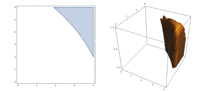
Figure 2. Left: Valid region of . Right: Valid region of .
- (1)
- •
: a similar argument as in the case shows that for each strongly Rayleigh variable . Again there are many ways to construct a strongly Rayleigh variable such that . For instance, the weight is transferred to , the weight is transferred to , the weight is transferred to , and the weight is transferred to . The PGF of is then . It is easily seen that the coefficients of the above PGF satisfy the Hutchinson-Kurtz condition (4.3). So . It is more difficult to find all strongly Rayleigh variables such that , since the conditions for a quartic function to have all real roots are more complicated [82].
- •
: consider the transference plan in Figure 3.
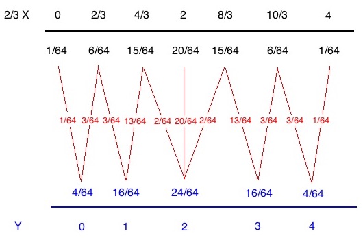
Figure 3. A transference plan from to . It is easy to see that the PGF of is , so and .
References
- [1] M. Aissen, A. Edrei, I. J. Schoenberg, and A. Whitney. On the generating functions of totally positive sequences. Proc. Nat. Acad. Sci. U. S. A., 37:303–307, 1951.
- [2] M. Aissen, I. J. Schoenberg, and A. Whitney. On the generating functions of totally positive sequences. I. J. Analyse Math., 2:93–103, 1952.
- [3] T. W. Anderson and S. M. Samuels. Some inequalities among binomial and Poisson probabilities. In Proc. Fifth Berkeley Sympos. Math. Statist. and Probability (Berkeley, Calif., 1965/66), pages Vol. I: Statistics, pp. 1–12. Univ. California Press, Berkeley, Calif., 1967.
- [4] T. Ando. Totally positive matrices. Linear Algebra Appl., 90:165–219, 1987.
- [5] K. Azuma. Weighted sums of certain dependent random variables. Tohoku Math. J. (2), 19:357–367, 1967.
- [6] A. Barbour, L. Holst, and S. Janson. Poisson approximation. 1992.
- [7] A. D. Barbour and P. Hall. On the rate of Poisson convergence. Math. Proc. Cambridge Philos. Soc., 95(3):473–480, 1984.
- [8] D. Berend and T. Tassa. Improved bounds on Bell numbers and on moments of sums of random variables. Probab. Math. Statist., 30(2):185–205, 2010.
- [9] P. J. Bickel and W. R. van Zwet. On a theorem of Hoeffding. In Asymptotic theory of statistical tests and estimation (Proc. Adv. Internat. Sympos., Univ. North Carolina, Chapel Hill, N.C., 1979), pages 307–324. Academic Press, New York-London-Toronto, Ont., 1980.
- [10] R. Biehler. Sur une classe d’équations algébriques dont toutes les racines sont réelles. J. Reine Angew. Math., 87:350–352, 1879.
- [11] P. Billingsley. Probability and measure. Wiley Series in Probability and Mathematical Statistics. John Wiley & Sons, Inc., New York, third edition, 1995.
- [12] L. Birgé. Estimation of unimodal densities without smoothness assumptions. Ann. Statist., 25(3):970–981, 1997.
- [13] W. Biscarri, S. D. Zhao, and R. J. Brunner. A simple and fast method for computing the Poisson binomial distribution function. Comput. Statist. Data Anal., 122:92–100, 2018.
- [14] S. G. Bobkov. Berry-Esseen bounds and Edgeworth expansions in the central limit theorem for transport distances. Probab. Theory Related Fields, 170(1-2):229–262, 2018.
- [15] P. J. Boland. The probability distribution for the number of successes in independent trials. Comm. Statist. Theory Methods, 36(5-8):1327–1331, 2007.
- [16] P. J. Boland and F. Proschan. The reliability of out of systems. Ann. Probab., 11(3):760–764, 1983.
- [17] P. J. Boland, H. Singh, and B. Cukic. Stochastic orders in partition and random testing of software. J. Appl. Probab., 39(3):555–565, 2002.
- [18] P. J. Boland, H. Singh, and B. Cukic. The stochastic precedence ordering with applications in sampling and testing. J. Appl. Probab., 41(1):73–82, 2004.
- [19] J. Borcea and P. Brändén. Applications of stable polynomials to mixed determinants: Johnson’s conjectures, unimodality, and symmetrized Fischer products. Duke Math. J., 143(2):205–223, 2008.
- [20] J. Borcea and P. Brändén. Pólya-Schur master theorems for circular domains and their boundaries. Ann. of Math. (2), 170(1):465–492, 2009.
- [21] J. Borcea, P.r Brändén, and T. M. Liggett. Negative dependence and the geometry of polynomials. J. Amer. Math. Soc., 22(2):521–567, 2009.
- [22] F. Brenti. Unimodal, log-concave and Pólya frequency sequences in combinatorics. Mem. Amer. Math. Soc., 81(413):viii+106, 1989.
- [23] F. Brenti. Unimodal polynomials arising from symmetric functions. Proc. Amer. Math. Soc., 108(4):1133–1141, 1990.
- [24] W. E. Briggs. Zeros and factors of polynomials with positive coefficients and protein-ligand binding. Rocky Mountain J. Math., 15(1):75–89, 1985.
- [25] T. Broderick, J. Pitman, and M. I. Jordan. Feature allocations, probability functions, and paintboxes. Bayesian Anal., 8(4):801–836, 2013.
- [26] S. Chatterjee, P. Diaconis, and E. Meckes. Exchangeable pairs and Poisson approximation. Probab. Surv., 2:64–106, 2005.
- [27] L. H. Y. Chen and Q-M Shao. A non-uniform Berry-Esseen bound via Stein’s method. Probab. Theory Related Fields, 120(2):236–254, 2001.
- [28] L. H. Y. Chen and Q-M Shao. Stein’s method for normal approximation. In An introduction to Stein’s method, volume 4 of Lect. Notes Ser. Inst. Math. Sci. Natl. Univ. Singap., pages 1–59. Singapore Univ. Press, Singapore, 2005.
- [29] S. X. Chen and J. S. Liu. Statistical applications of the Poisson-binomial and conditional Bernoulli distributions. Statist. Sinica, 7(4):875–892, 1997.
- [30] X-H Chen, A. P. Dempster, and J. S. Liu. Weighted finite population sampling to maximize entropy. Biometrika, 81(3):457–469, 1994.
- [31] K. P. Choi and A-H Xia. Approximating the number of successes in independent trials: binomial versus Poisson. Ann. Appl. Probab., 12(4):1139–1148, 2002.
- [32] J. N. Darroch. On the distribution of the number of successes in independent trials. Ann. Math. Statist., 35, 1964.
- [33] C. Daskalakis, I. Diakonikolas, R. O’Donnell, R. A. Servedio, and L-Y Tan. Learning sums of independent integer random variables. In Foundations of Computer Science (FOCS), 2013 IEEE 54th Annual Symposium, pages 217–226, 2013.
- [34] C. Daskalakis, I. Diakonikolas, and R. A. Servedio. Learning Poisson binomial distributions. Algorithmica, 72(1):316–357, 2015.
- [35] C. Daskalakis and C. Papadimitriou. Sparse covers for sums of indicators. Probab. Theory Related Fields, 162(3-4):679–705, 2015.
- [36] L. Devroye and G. Lugosi. Combinatorial methods in density estimation. Springer Series in Statistics. Springer-Verlag, New York, 2001.
- [37] I. Diakonikolas, D. M. Kane, and A. Stewart. The Fourier transform of Poisson multinomial distributions and its algorithmic applications. In STOC’16—Proceedings of the 48th Annual ACM SIGACT Symposium on Theory of Computing, pages 1060–1073. ACM, New York, 2016.
- [38] I. Diakonikolas, D. M. Kane, and A. Stewart. Optimal learning via the Fourier transform for sums of independent integer random variables. In Conference on Learning Theory, pages 831–849, 2016.
- [39] I. Diakonikolas, D. M. Kane, and A. Stewart. Properly learning Poisson binomial distributions in almost polynomial time. In Conference on Learning Theory, pages 850–878, 2016.
- [40] D. Duffie, L. Saita, and K. Wang. Multi-period corporate default prediction with stochastic covariates. Journal of Financial Economics, 83(3):635–665, 2007.
- [41] W. Ehm. Binomial approximation to the Poisson binomial distribution. Statist. Probab. Lett., 11(1):7–16, 1991.
- [42] S. Fallat, C. R. Johnson, and A. D. Sokal. Total positivity of sums, Hadamard products and Hadamard powers: results and counterexamples. Linear Algebra Appl., 520:242–259, 2017.
- [43] M. Fernández and S. Williams. Closed-form expression for the poisson-binomial probability density function. IEEE Transactions on Aerospace and Electronic Systems, 46(2):803–817, 2010.
- [44] M. F. Fernandez and T. Aridgides. Measures for evaluating sea mine identification processing performance and the enhancements provided by fusing multisensor/multiprocess data via an M-out-of-N voting scheme. In Detection and Remediation Technologies for Mines and Minelike Targets VIII, volume 5089, pages 425–436, 2003.
- [45] M. H. Gail, J. H. Lubin, and L. V. Rubinstein. Likelihood calculations for matched case-control studies and survival studies with tied death times. Biometrika, 68(3):703–707, 1981.
- [46] M. Gasca and J. M. Peña. Total positivity and Neville elimination. Linear Algebra Appl., 165:25–44, 1992.
- [47] S. Ghosh, T. M. Liggett, and R. Pemantle. Multivariate CLT follows from strong Rayleigh property. In 2017 Proceedings of the Fourteenth Workshop on Analytic Algorithmics and Combinatorics (ANALCO), pages 139–147. SIAM, Philadelphia, PA, 2017.
- [48] L. J. Gleser. On the distribution of the number of successes in independent trials. Ann. Proba., 3:182–188, 1975.
- [49] L. Goldstein. Bounds on the constant in the mean central limit theorem. Ann. Probab., 38(4):1672–1689, 2010.
- [50] D. Handelman. Arguments of zeros of highly log concave polynomials. Rocky Mountain J. Math., 43(1):149–177, 2013.
- [51] C. Hermite. Sur le nombre des racines d’une équation algébrique comprises entre des limites données. J. Reine Angew. Math., 52:39–51, 1856.
- [52] E. Hillion and O. Johnson. A proof of the Shepp-Olkin entropy concavity conjecture. Bernoulli, 23(4B):3638–3649, 2017.
- [53] W. Hoeffding. On the distribution of the number of successes in independent trials. The Annals of Mathematical Statistics, 27(3):713–721, 1956.
- [54] W. Hoeffding. Probability inequalities for sums of bounded random variables. J. Amer. Statist. Assoc., 58:13–30, 1963.
- [55] O. Holtz and M. Tyaglov. Structured matrices, continued fractions, and root localization of polynomials. SIAM Rev., 54(3):421–509, 2012.
- [56] Y-L Hong. On computing the distribution function for the Poisson binomial distribution. Comput. Statist. Data Anal., 59:41–51, 2013.
- [57] Y-L Hong, W. Q. Meeker, and J. D. McCalley. Prediction of remaining life of power transformers based on left truncated and right censored lifetime data. Ann. Appl. Stat., 3(2):857–879, 2009.
- [58] J. I. Hutchinson. On a remarkable class of entire functions. Trans. Amer. Math. Soc., 25(3):325–332, 1923.
- [59] S. Janson. Coupling and Poisson approximation. Acta Appl. Math., 34(1-2):7–15, 1994.
- [60] K. Jogdeo and S. M. Samuels. Monotone convergence of binomial probabilities and a generalization of Ramanujan’s equation. Ann. Math. Statist., 39(4):1191–1195, 1968.
- [61] O. M. Katkova and A. M. Vishnyakova. A sufficient condition for a polynomial to be stable. J. Math. Anal. Appl., 347(1):81–89, 2008.
- [62] V. P. Kostov and B. Shapiro. Hardy-Petrovitch-Hutchinson’s problem and partial theta function. Duke Math. J., 162(5):825–861, 2013.
- [63] D. C. Kurtz. A sufficient condition for all the roots of a polynomial to be real. Amer. Math. Monthly, 99(3):259–263, 1992.
- [64] L. Le Cam. An approximation theorem for the Poisson binomial distribution. Pacific J. Math., 10:1181–1197, 1960.
- [65] T. M. Liggett. Approximating multiples of strong Rayleigh random variables. 2018. Unpublished manuscript.
- [66] A. W. Marshall, I. Olkin, and B. C. Arnold. Inequalities: theory of majorization and its applications. Springer Series in Statistics. Springer, New York, second edition, 2011.
- [67] K. Neammanee. On the constant in the nonuniform version of the Berry-Esseen theorem. Int. J. Math. Math. Sci., (12):1951–1967, 2005.
- [68] J. Nedelman and T. Wallenius. Bernoulli trials, Poisson trials, surprising variances, and Jensen’s inequality. Amer. Statist., 40(4):286–289, 1986.
- [69] C. P. Niculescu. Interpolating Newton’s inequalities. Bull. Math. Soc. Sci. Math. Roumanie (N.S.), 47(95)(1-2):67–83, 2004.
- [70] S. Y. Novak. Poisson approximation. Probab. Surv., 16:228–276, 2019.
- [71] M. Okamoto. Some inequalities relating to the partial sum of binomial probabilities. Ann. Inst. Statist. Math., 10:29–35, 1958.
- [72] L. Paditz. On the analytical structure of the constant in the nonuniform version of the Esseen inequality. Statistics, 20(3):453–464, 1989.
- [73] E. A. Peköz, A. Röllin, V. Čekanavičius, and M. Shwartz. A three-parameter binomial approximation. J. Appl. Probab., 46(4):1073–1085, 2009.
- [74] R. Pemantle. Towards a theory of negative dependence. volume 41, pages 1371–1390. 2000. Probabilistic techniques in equilibrium and nonequilibrium statistical physics.
- [75] V. V. Petrov. A bound for the deviation of the distribution of a sum of independent random variables from the normal law. Dokl. Akad. Nauk SSSR, 160:1013–1015, 1965.
- [76] V. V. Petrov. Sums of independent random variables. Springer-Verlag, New York-Heidelberg, 1975. Translated from the Russian by A. A. Brown, Ergebnisse der Mathematik und ihrer Grenzgebiete, Band 82.
- [77] J. Pitman. Probability. Springer Texts in Statistics. Springer-Verlag New York, 1993.
- [78] J. Pitman. Probabilistic bounds on the coefficients of polynomials with only real zeros. J. Combin. Theory Ser. A, 77(2):279–303, 1997.
- [79] M. L. Platonov. Combinatorial numbers of a class of mappings and their applications. “Nauka”, Moscow, 1979.
- [80] G. Pledger and F. Proschan. Comparisons of order statistics and of spacings from heterogeneous distributions. In Optimizing methods in statistics (Proc. Sympos., Ohio State Univ., Columbus, Ohio, 1971), pages 89–113, 1971.
- [81] S. D. Poisson. Recherches sur la probabilité des jugements en matière criminelle et en matière civile. Bachelier, 1837.
- [82] E. L. Rees. Graphical Discussion of the Roots of a Quartic Equation. Amer. Math. Monthly, 29(2):51–55, 1922.
- [83] K. Rietsch. Totally positive Toeplitz matrices and quantum cohomology of partial flag varieties. J. Amer. Math. Soc., 16(2):363–392, 2003.
- [84] E. Rio. Upper bounds for minimal distances in the central limit theorem. Ann. Inst. Henri Poincaré Probab. Stat., 45(3):802–817, 2009.
- [85] A. Röllin. Translated Poisson approximation using exchangeable pair couplings. Ann. Appl. Probab., 17(5-6):1596–1614, 2007.
- [86] B. Roos. Asymptotic and sharp bounds in the Poisson approximation to the Poisson-binomial distribution. Bernoulli, 5(6):1021–1034, 1999.
- [87] B. Roos. Binomial approximation to the Poisson binomial distribution: the Krawtchouk expansion. Teor. Veroyatnost. i Primenen., 45(2):328–344, 2000.
- [88] P. R. Rosenbaum. Observational studies. Springer Series in Statistics. Springer-Verlag, New York, second edition, 2002.
- [89] E. Rosenman. Some new results for Poisson binomial models. 2018. arXiv:1907.09053.
- [90] S. Rosset. Normalized symmetric functions, Newton’s inequalities and a new set of stronger inequalities. Amer. Math. Monthly, 96(9):815–819, 1989.
- [91] S. M. Samuels. On the number of successes in independent trials. Ann. Math. Statist., 36:1272–1278, 1965.
- [92] N. Schumacher. Binomial option pricing with nonidentically distributed returns and its implications. Mathematical and computer modelling, 29(10-12):121–143, 1999.
- [93] L. A. Shepp and I. Olkin. Entropy of the sum of independent Bernoulli random variables and of the multinomial distribution. In Contributions to probability, pages 201–206. Academic Press, New York-London, 1981.
- [94] I. S. Shiganov. Refinement of the upper bound of a constant in the remainder term of the central limit theorem. In Stability problems for stochastic models (Moscow, 1982), pages 109–115. Vsesoyuz. Nauchno-Issled. Inst. Sistem. Issled., Moscow, 1982.
- [95] Max Skipper. A Pólya approximation to the Poisson-binomial law. J. Appl. Probab., 49(3):745–757, 2012.
- [96] R. P. Stanley. Log-concave and unimodal sequences in algebra, combinatorics, and geometry. In Graph theory and its applications: East and West (Jinan, 1986), volume 576 of Ann. New York Acad. Sci., pages 500–535. New York Acad. Sci., New York, 1989.
- [97] C. Stein. Application of Newton’s identities to a generalized birthday problem and to the Poisson binomial distribution, 1990. Technical Report 354, Department of Statistics, Stanford University.
- [98] G. Stengle. A nullstellensatz and a positivstellensatz in semialgebraic geometry. Math. Ann., 207:87–97, 1974.
- [99] B. Sturmfels. Solving systems of polynomial equations, volume 97 of CBMS Regional Conference Series in Mathematics. Published for the Conference Board of the Mathematical Sciences, Washington, DC; by the American Mathematical Society, Providence, RI, 2002.
- [100] A. Tejada and J. Arnold. The role of Poisson’s binomial distribution in the analysis of TEM images. Ultramicroscopy, 111(11):1553–1556, 2011.
- [101] P. Thongtha and K. Neammanee. Refinement on the constants in the non-uniform version of the Berry-Esseen theorem. Thai J. Math., 5(1):1–13, 2007.
- [102] P. van Beek. An application of Fourier methods to the problem of sharpening the Berry-Esseen inequality. Z. Wahrscheinlichkeitstheorie und Verw. Gebiete, 23:187–196, 1972.
- [103] C. Villani. Optimal transport: Old and new, volume 338 of Grundlehren der Mathematischen Wissenschaften [Fundamental Principles of Mathematical Sciences]. Springer-Verlag, Berlin, 2009.
- [104] Y. H. Wang. On the number of successes in independent trials. Statist. Sinica, 3(2):295–312, 1993.
- [105] Wikipedia. Cubic function. https://en.wikipedia.org/wiki/Cubicfunction.
- [106] B. Xia and L. Yang. A new result on the -irreducibility of binding polynomials. Comput. Math. Appl., 48(12):1811–1817, 2004.
- [107] M-C Xu and N. Balakrishnan. On the convolution of heterogeneous Bernoulli random variables. J. Appl. Probab., 48(3):877–884, 2011.
- [108] L-H Zhi and Z-J Liu. -irreducibility of binding polynomials. Comput. Math. Appl., 38(2):1–10, 1999.