KMT-2016-BLG-1836Lb: A Super-Jovian Planet From A High-Cadence Microlensing FieldpySIS (Albrow et al. 2009), pyDIA (doi:10.5281/zenodo.268049), emcee (Foreman-Mackey et al. 2013), DoPhot (Schechter et al. 1993)

A standard binary lens model has seven parameters to calculate the magnification, $A(t)$. Three ($t_{0}$, $u_{0}$, $t_{\rm E}$) of these parameters describe a point-lens event (Paczyński 1986): the time of the maximum magnification, the minimum impact parameter in units of the angular Einstein radius $\theta_{\rm E}$, and the Einstein radius crossing time. The next three ($q$, $s$, $\alpha$) define the binary geometry: the binary mass ratio, the projected separation between the binary components normalized to the Einstein radius, and the angle between the source trajectory and the binary axis in the lens plane. The last parameter is the source radius normalized by the Einstein radius, $\rho=\theta_{*}/\theta_{\rm E}$. In addition, for each data set $i$, two flux parameters ($f_{{\rm S},i}$, $f_{{\rm B},i}$) represent the flux of the source star and the blend flux. The observed flux, $f_{i}(t)$, calculated from the model is

We locate the $\chi^{2}$ minima by a searching over a grid of parameters ($\log s,\log q,\alpha$). The grids consist of 21 values equally spaced between $-1\leq\log s\leq 1$, 10 values equally spaced between $0^{\circ}\leq\alpha<360^{\circ}$, and 51 values equally spaced between $-5\leq\log q\leq 0$. For each set of ($\log s,\log q,\alpha$), we fix $\log q$, $\log s$, $\rho=0.001$, and free $t_{0},u_{0},t_{\rm E},\alpha$. We find the minimum $\chi^{2}$ by Markov chain Monte Carlo (MCMC) $\chi^{2}$ minimization using the emcee ensemble sampler (Foreman-Mackey et al. 2013). The upper panel of Figure 2 shows the $\chi^{2}$ distribution in the ($\log s,\log q$) plane from the grid search, which indicates the distinct minima are within $-0.3\leq\log s\leq 0.3$ and $-5\leq\log q\leq-1$. We therefore conduct a denser grid search, which consists of 61 values equally spaced between $-0.3\leq\log s\leq 0.3$, 10 values equally spaced between $0^{\circ}\leq\alpha<360^{\circ}$, and 41 values equally spaced between $-5\leq\log q\leq-1$. As a result, we find four distinct minima and label them as “A”, “B”, “C” and “D” in the lower panel of Figure 2. We then investigate the best-fit model with all free parameters. Table 1 shows best-fit parameters of the four solutions from MCMC. The MCMC results show that the solution “B” is the best-fit model, while the solution “A” is disfavored by $\Delta\chi^{2}\sim 16$. We note that these two solutions are related by the so-called close-wide degeneracy and approximately take $s\leftrightarrow s^{-1}$ (Griest & Safizadeh 1998; Dominik 1999), so we label them by “Close” (solution B, $s<1$) and “Wide” (solution A, $s>1$) in the following analysis. The solutions “C” and “D” are disfavored by $\Delta\chi^{2}\sim 474$ and $\Delta\chi^{2}\sim 235$, respectively, so we exclude these two solutions. For both the solutions “Close” and “Wide”, the data are consistent with a point-source model within $\sim 2\sigma$ level, and the upper limit for $\rho$ is $2.0\times 10^{-3}$ for the solution “Close” and $2.8\times 10^{-3}$ for the solution “Wide”. The best-fit model curves for the two solutions are shown in Figure 1, and their magnification maps are shown in Figure 3.

In addition, we check whether the fit further improves by considering the microlens-parallax effect,

where $(\pi_{\rm rel},\bm{\mu}_{\rm rel})$ are the lens-source relative (parallax, proper motion), which is caused by the orbital acceleration of Earth (Gould 1992). We also fit $u_{0}>0$ and $u_{0}<0$ solutions to consider the “ecliptic degeneracy” (Skowron et al. 2011). To facilitate the further discussion of these solutions, we label them by $C_{\pm}$ or $W_{\pm}$. The letter stands for “Close” ($s<1$) or “Wide” ($s>1$), while the subscript refers to the sign of $u_{0}$. The addition of parallax to the model does not significantly improve the fit, providing an improvement of $\Delta\chi^{2}<3.0$ for the $C_{\pm}$ solutions and $\Delta\chi^{2}<1.7$ for the $W_{\pm}$ solutions. However, we find that the east component of the parallax vector $\pi_{\rm E,E}$ is well constrained for all the solutions, while the constraint on the north component $\pi_{\rm E,N}$ is considerably weaker. Table 2 shows best-fit parameters of the standard binary-lens model, $C_{\pm}$ and $W_{\pm}$ solutions, and Figure 4 shows the likelihood distribution of $(\pi_{\rm E,N},\pi_{\rm E,E})$ from MCMC.

The total magnification of a binary-source event is the superposition of two point-lens events,

where $f_{{\rm i},\lambda}$ (${\rm i}=1,2$) is the flux at wavelength $\lambda$ of each source and $A_{\lambda}$ is total magnification. We search for 1L2S solutions using MCMC, and the best-fit model is disfavored by $\Delta\chi^{2}\sim 38$ compared to the binary-lens “Wide” model (see Table 3). Figure 5 presents their cumulative distribution of $\chi^{2}$ differences, which shows the $\chi^{2}$ differences are mainly from $\pm 20$ days from the peak, rather than outliers. We also consider the microlens-parallax effect, but the improvement is very minor with $\Delta\chi^{2}\sim 1.4$. Thus, we exclude the 1L2S solution.

To further estimate the angular Einstein radius $\theta_{\rm E}=\theta_{*}/\rho$, we estimate the angular radius $\theta_{*}$ of the source by locating the source on a CMD (Yoo et al. 2004). We calibrate the KMTC02 pyDIA reduction to the OGLE-III star catalog (Szymański et al. 2011) and construct a $V-I$ versus $I$ CMD using stars within a $2^{\prime}\times 2^{\prime}$ square centered on the event (see Figure 6). The red giant clump is at $(V-I,I)_{\rm cl}=(2.64\pm 0.01,16.30\pm 0.02)$, whereas the source is at $(V-I,I)_{\rm S}=(2.40\pm 0.07,22.12\pm 0.05)$ for the Wide solution and $(V-I,I)_{\rm S}=(2.40\pm 0.07,22.01\pm 0.05)$ for the Close solution. We adopt the intrinsic color and de-reddened magnitude of the red giant clump $(V-I,I)_{\rm cl,0}=(1.06,14.42)$ from Bensby et al. 2013 and Nataf et al. 2016, and then we derive the intrinsic color and de-reddened brightness of the source as $(V-I,I)_{\rm S,0}=(0.82\pm 0.08,20.24\pm 0.06)$ for the Wide solution and $(V-I,I)_{\rm S,0}=(0.82\pm 0.08,20.13\pm 0.06)$ for the close solution. These values suggest the source is either a late-G or early-K type main-sequence star. Using the color/surface-brightness relation for dwarfs and sub-giants of Adams et al. 2018, we obtain

For KMT-2016-BLG-1836, the microlens source is too faint to measure its proper motion either from Gaia (Li et al. 2019, e.g.,) or from ground-based data (Shvartzvald et al. 2019, e.g.,). However, we can still estimate the source proper motion by the proper-motion distribution of “bulge” stars in the Gaia DR2 catalog (Gaia Collaboration et al. 2016; Gaia Collaboration et al. 2018). We examine a Gaia CMD using the stars within 1 arcmin and derive the proper motion (in the Sun frame) of red giant branch stars ($G<18.6;B_{p}-R_{p}>2.2$). We remove one outlier and obtain (in the Sun frame)

For a lensing object, the total mass is related to $\theta_{\rm E}$ and $\pi_{\rm E}$ by (Gould 1992; Gould 2000)

and its distance by

where $\kappa\equiv 4G/(c^{2}\mathrm{AU})=8.144$ mas$/M_{\odot}$, $\pi_{\rm S}=\mathrm{AU}/D_{\rm S}$ is the source parallax, and $D_{\rm S}$ is the source distance. In the present case, neither $\theta_{\rm E}$ nor $\pi_{\rm E}$ is unambiguously measured, so we conduct a Bayesian analysis to estimate the physical parameters of the lens systems.

For each solution of $C_{\pm}$ and $W_{\pm}$, we first create a sample of $10^{9}$ simulated events from the Galactic model of Zhu et al. 2017. We also choose the initial mass function of Kroupa 2001 and $1.3M_{\odot}$ for the upper end of the initial mass function. The only exception is that we draw the source proper motions from a Gaussian distribution with the parameters that were derived in Section IV.2. For each simulated event $i$ of solution $k$, we then weight it by

where $\Gamma_{i,k}\varpropto\theta_{{\rm E},i,k}\times\mu_{{\rm rel},i,k}$ is the microlensing event rate, $\mathcal{L}_{i,k}(t_{\rm E}),\mathcal{L}_{i,k}(\bm{\pi}_{\rm E})$ are the likelihood of its inferred parameters $(t_{\rm E},\bm{\pi}_{\rm E})_{i,k}$ given the error distributions of these quantities derived from the MCMC for that solution

$b_{m,n}^{k}$ is the inverse covariance matrix of $\bm{\pi}_{{\rm E},k}$, and $(m,n)$ are dummy variables ranging over ($N,E$), and $\mathcal{L}_{i,k}(\theta_{\rm E})$ is the likelihood derived from the minimum $\chi^{2}$ for the lower envelope of the ($\chi^{2}$ vs. $\rho$) diagram from MCMC and the measured source angular radius $\theta_{*}$ from Section IV.1. Finally, we weight each solution by ${\rm exp}(-\Delta\chi^{2}_{k}/2)$, where $\Delta\chi^{2}_{k}$ is the $\chi^{2}$ difference between the $k$th solution and the best-fit solution.

Table 4 shows the resulting lens properties and relative weights for each solution, and the combined results. We find that the “Wide” solutions are significantly favored because they are preferred by a factor of $\sim{\rm exp}(14/2)\sim 10^{3}$ from the $\chi^{2}$ weight, while the “Wide” solutions also have slightly higher Galactic model likelihood. The net effect is that the resulting combined solution is basically the same as the wide solution. The Bayesian analysis yields a host mass of $M_{\rm host}=0.49_{-0.25}^{+0.38}~M_{\odot}$, a planet mass of $M_{\rm planet}=2.2_{-1.1}^{+1.9}~M_{J}$, and a host-planet projected separation $r_{\perp}=3.5_{-0.9}^{+1.1}~{\rm AU}$, which indicates the planet is a super-Jovian planet well beyond the snow line of an M/K dwarf star (assuming a snow line radius $r_{\rm SL}=2.7(M/M_{\odot})$ AU, Kennedy & Kenyon 2008). For each solution, the resulting distributions of the lens host-mass $M_{\rm host}$ and the lens distance $D_{\rm L}$ are shown in Figures 7 and 8, respectively. The resulting combined distributions of the lens properties are shown in Figure 9.

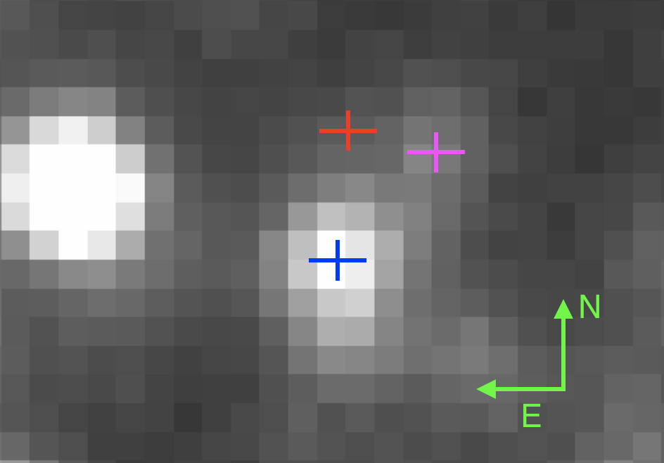
The light curve analysis shows the blended light for the pySIS light curve is $I_{\rm B}\sim 18.25$. To investigate the blend, we check the higher-resolution $i$-band images (pixel scale $0.185^{\prime\prime}$, FWHM $\sim 0.6^{\prime\prime}$) taken from the Canada-France-Hawaii Telescope (CFHT) located at the Maunakea Observatories in 2018 (Zang et al. 2018b). We identify the source position in the CFHT images from an astrometric transformation of the highly magnified KMTC02 images. We use DoPhot (Schechter et al. 1993) to identify nearby stars and do photometry. As a result, DoPhot identifies two stars within $1^{\prime\prime}$ (see Figure 10): an $I=18.18\pm 0.02$ star offset from the source by $0.88^{\prime\prime}$, and an $I=19.43\pm 0.05$ star offset by $0.61^{\prime\prime}$. Thus, the blend of pySIS light curve is from unrelated ambient stars. In addition, the total brightness of the source and the lens is fainter than the nearby $I=19.43\pm 0.05$ star.

From the CMD analysis and the Bayesian analysis, the source is a late-G or early-K dwarf and the lens is probably an M/K dwarf. Thus, the lens and source may have approximately equal brightness in the near-infrared, therefore follow-up adaptive-optics (AO) observations can potentially strongly constrain the lens brightness and thus the mass and distance of the planetary system (Batista et al. 2015; Bennett et al. 2015; Bhattacharya et al. 2018). In addition, our Bayesian analysis shows that the lens-source relative proper motion is $\mu_{\rm rel}=3.3_{-0.9}^{+1.5}{\rm mas\,yr^{-1}}$, so the lens and source will be separated by about 40 mas by 2028. Thus, the source and lens can be resolved by the first AO light on next-generation (30 m) telescopes, which have a resolution $\theta\sim 14(D/30{\rm m})^{-1}$ mas in $H$ band.

References

- Adams et al. (2018) Adams, A. D., Boyajian, T. S., & von Braun, K. 2018, MNRAS, 473, 3608
- Alard & Lupton (1998) Alard, C., & Lupton, R. H. 1998, ApJ, 503, 325
- Albrow et al. (2009) Albrow, M. D., Horne, K., Bramich, D. M., et al. 2009, MNRAS, 397, 2099
- Batista et al. (2015) Batista, V., Beaulieu, J.-P., Bennett, D. P., et al. 2015, ApJ, 808, 170
- Bennett et al. (2008) Bennett, D. P., Bond, I. A., Udalski, A., et al. 2008, ApJ, 684, 663
- Bennett et al. (2015) Bennett, D. P., Bhattacharya, A., Anderson, J., et al. 2015, ApJ, 808, 169
- Bensby et al. (2013) Bensby, T., Yee, J. C., Feltzing, S., et al. 2013, A&A, 549, A147
- Bhattacharya et al. (2018) Bhattacharya, A., Beaulieu, J. P., Bennett, D. P., et al. 2018, AJ, 156, 289
- Bond et al. (2004) Bond, I. A., Udalski, A., Jaroszyński, M., et al. 2004, ApJ, 606, L155
- Calchi Novati et al. (2015) Calchi Novati, S., Gould, A., Udalski, A., et al. 2015, ApJ, 804, 20
- Calchi Novati et al. (2018) Calchi Novati, S., Skowron, J., Jung, Y. K., et al. 2018, AJ, 155, 261
- Calchi Novati et al. (2019) Calchi Novati, S., Suzuki, D., Udalski, A., et al. 2019, AJ, 157, 121
- Dominik (1999) Dominik, M. 1999, A&A, 349, 108
- Foreman-Mackey et al. (2013) Foreman-Mackey, D., Hogg, D. W., Lang, D., & Goodman, J. 2013, PASP, 125, 306
- Gaia Collaboration et al. (2016) Gaia Collaboration, Prusti, T., de Bruijne, J. H. J., et al. 2016, A&A, 595, A1
- Gaia Collaboration et al. (2018) Gaia Collaboration, Brown, A. G. A., Vallenari, A., et al. 2018, A&A, 616, A1
- Gaudi (1998) Gaudi, B. S. 1998, ApJ, 506, 533
- Gould (1992) Gould, A. 1992, ApJ, 392, 442
- Gould (2000) —. 2000, ApJ, 542, 785
- Gould et al. (2013) Gould, A., Carey, S., & Yee, J. 2013, Spitzer Microlens Planets and Parallaxes, Spitzer Proposal, ,
- Gould et al. (2014) —. 2014, Galactic Distribution of Planets from Spitzer Microlens Parallaxes, Spitzer Proposal, ,
- Gould et al. (2016) —. 2016, Galactic Distribution of Planets Spitzer Microlens Parallaxes, Spitzer Proposal, ,
- Gould & Horne (2013) Gould, A., & Horne, K. 2013, ApJ, 779, L28
- Gould & Loeb (1992) Gould, A., & Loeb, A. 1992, ApJ, 396, 104
- Gould et al. (2015a) Gould, A., Yee, J., & Carey, S. 2015a, Degeneracy Breaking for K2 Microlens Parallaxes, Spitzer Proposal, ,
- Gould et al. (2015b) —. 2015b, Galactic Distribution of Planets From High-Magnification Microlensing Events, Spitzer Proposal, ,
- Gould et al. (2018) Gould, A., Yee, J., Carey, S., & Shvartzvald, Y. 2018, The Galactic Distribution of Planets via Spitzer Microlensing Parallax, Spitzer Proposal, ,
- Gould et al. (2019) Gould, A., Ryu, Y.-H., Calchi Novati, S., et al. 2019, arXiv e-prints, arXiv:1906.11183
- Griest & Safizadeh (1998) Griest, K., & Safizadeh, N. 1998, ApJ, 500, 37
- Han (2002) Han, C. 2002, ApJ, 564, 1015
- Han et al. (2017a) Han, C., Udalski, A., Gould, A., et al. 2017a, AJ, 154, 133
- Han et al. (2017b) —. 2017b, AJ, 154, 223
- Han et al. (2018a) Han, C., Bond, I. A., Gould, A., et al. 2018a, AJ, 156, 226
- Han et al. (2018b) Han, C., Hirao, Y., Udalski, A., et al. 2018b, AJ, 155, 211
- Han et al. (2019a) Han, C., Udalski, A., Gould, A., et al. 2019a, arXiv e-prints, arXiv:1911.11953
- Han et al. (2019b) Han, C., Bennett, D. P., Udalski, A., et al. 2019b, AJ, 158, 114
- Han et al. (2019c) Han, C., Lee, C.-U., Udalski, A., et al. 2019c, arXiv e-prints, arXiv:1909.04854
- Han et al. (2019d) Han, C., Yee, J. C., Udalski, A., et al. 2019d, AJ, 158, 102
- Henderson et al. (2014) Henderson, C. B., Gaudi, B. S., Han, C., et al. 2014, ApJ, 794, 52
- Henderson et al. (2016) Henderson, C. B., Poleski, R., Penny, M., et al. 2016, PASP, 128, 124401
- Holtzman et al. (1998) Holtzman, J. A., Watson, A. M., Baum, W. A., et al. 1998, AJ, 115, 1946
- Hwang et al. (2018a) Hwang, K. H., Kim, H. W., Kim, D. J., et al. 2018a, Journal of Korean Astronomical Society, 51, 197
- Hwang et al. (2018b) Hwang, K.-H., Udalski, A., Shvartzvald, Y., et al. 2018b, AJ, 155, 20
- Hwang et al. (2019) Hwang, K.-H., Ryu, Y.-H., Kim, H.-W., et al. 2019, AJ, 157, 23
- Ida & Lin (2004) Ida, S., & Lin, D. N. C. 2004, ApJ, 604, 388
- Jung et al. (2018a) Jung, Y. K., Hwang, K.-H., Ryu, Y.-H., et al. 2018a, AJ, 156, 208
- Jung et al. (2018b) Jung, Y. K., Udalski, A., Gould, A., et al. 2018b, AJ, 155, 219
- Jung et al. (2019a) Jung, Y. K., Gould, A., Zang, W., et al. 2019a, AJ, 157, 72
- Jung et al. (2019b) Jung, Y. K., Gould, A., Udalski, A., et al. 2019b, AJ, 158, 28
- Kennedy & Kenyon (2008) Kennedy, G. M., & Kenyon, S. J. 2008, ApJ, 673, 502
- Kim et al. (2018a) Kim, D.-J., Kim, H.-W., Hwang, K.-H., et al. 2018a, AJ, 155, 76
- Kim et al. (2018b) Kim, H.-W., Hwang, K.-H., Kim, D.-J., et al. 2018b, ArXiv e-prints, arXiv:1804.03352
- Kim et al. (2018c) —. 2018c, AJ, 155, 186
- Kim et al. (2016) Kim, S.-L., Lee, C.-U., Park, B.-G., et al. 2016, Journal of Korean Astronomical Society, 49, 37
- Kroupa (2001) Kroupa, P. 2001, MNRAS, 322, 231
- Li et al. (2019) Li, S. S., Zang, W., Udalski, A., et al. 2019, MNRAS, 488, 3308
- Mao & Paczynski (1991) Mao, S., & Paczynski, B. 1991, ApJ, 374, L37
- Mróz et al. (2017) Mróz, P., Han, C., and, et al. 2017, AJ, 153, 143
- Mróz et al. (2019) Mróz, P., Udalski, A., Skowron, J., et al. 2019, ApJS, 244, 29
- Nataf et al. (2016) Nataf, D. M., Gonzalez, O. A., Casagrande, L., et al. 2016, MNRAS, 456, 2692
- Paczyński (1986) Paczyński, B. 1986, ApJ, 304, 1
- Ryu et al. (2018) Ryu, Y.-H., Yee, J. C., Udalski, A., et al. 2018, AJ, 155, 40
- Ryu et al. (2019a) Ryu, Y.-H., Navarro, M. G., Gould, A., et al. 2019a, arXiv e-prints, arXiv:1905.04870
- Ryu et al. (2019b) Ryu, Y.-H., Hwang, K.-H., Gould, A., et al. 2019b, AJ, 158, 151
- Ryu et al. (2019c) Ryu, Y.-H., Udalski, A., Yee, J. C., et al. 2019c, arXiv e-prints, arXiv:1905.08148
- Schechter et al. (1993) Schechter, P. L., Mateo, M., & Saha, A. 1993, PASP, 105, 1342
- Shin et al. (2019) Shin, I. G., Ryu, Y. H., Yee, J. C., et al. 2019, AJ, 157, 146
- Shvartzvald et al. (2017) Shvartzvald, Y., Yee, J. C., Calchi Novati, S., et al. 2017, ApJ, 840, L3
- Shvartzvald et al. (2019) Shvartzvald, Y., Yee, J. C., Skowron, J., et al. 2019, AJ, 157, 106
- Skowron et al. (2011) Skowron, J., Udalski, A., Gould, A., et al. 2011, ApJ, 738, 87
- Skowron et al. (2018) Skowron, J., Ryu, Y.-H., Hwang, K.-H., et al. 2018, Acta Astron., 68, 43
- Street et al. (2016) Street, R. A., Udalski, A., Calchi Novati, S., et al. 2016, ApJ, 819, 93
- Sumi et al. (2013) Sumi, T., Bennett, D. P., Bond, I. A., et al. 2013, ApJ, 778, 150
- Suzuki et al. (2016) Suzuki, D., Bennett, D. P., Sumi, T., et al. 2016, ApJ, 833, 145
- Suzuki et al. (2018) Suzuki, D., Bennett, D. P., Ida, S., et al. 2018, ApJ, 869, L34
- Szymański et al. (2011) Szymański, M. K., Udalski, A., Soszyński, I., et al. 2011, Acta Astron., 61, 83
- Udalski et al. (2005) Udalski, A., Jaroszyński, M., Paczyński, B., et al. 2005, ApJ, 628, L109
- Udalski et al. (2018) Udalski, A., Ryu, Y.-H., Sajadian, S., et al. 2018, Acta Astron., 68, 1
- Yoo et al. (2004) Yoo, J., DePoy, D. L., Gal-Yam, A., et al. 2004, ApJ, 603, 139
- Zang et al. (2018a) Zang, W., Hwang, K.-H., Kim, H.-W., et al. 2018a, AJ, 156, 236
- Zang et al. (2018b) Zang, W., Penny, M. T., Zhu, W., et al. 2018b, PASP, 130, 104401
- Zhu et al. (2017) Zhu, W., Udalski, A., Calchi Novati, S., et al. 2017, AJ, 154, 210