todoGreenrgb0.0, 0.5, 0.0
From canyons to valleys: Numerically continuing sticky hard sphere clusters to the landscapes of smoother potentials
Abstract
We study the energy landscapes of particles with short-range attractive interactions as the range of the interactions increases. Starting with the set of local minima for hard spheres that are “sticky”, i.e. they interact only when their surfaces are exactly in contact, we use numerical continuation to evolve the local minima (clusters) as the range of the potential increases, using both the Lennard-Jones and Morse families of interaction potentials. As the range increases, clusters merge, until at long ranges only one or two clusters are left. We compare clusters obtained by continuation with different potentials and find that for short and medium ranges, up to about 30% of particle diameter, the continued clusters are nearly identical, both within and across families of potentials. For longer ranges the clusters vary significantly, with more variation between families of potentials than within a family. We analyze the mechanisms behind the merge events, and find that most rearrangements occur when a pair of non-bonded particles comes within the range of the potential. An exception occurs for nonharmonic clusters, those that have a zero eigenvalue in their Hessian, which undergo a more global rearrangement.
I Introduction
Metastable states of a system of interacting particles determine much of the system’s behaviour, yet they can be difficult to study because they are sensitive to the interaction potential between the particles potentialsAS; potentials2; Wales:2003. For mesoscale particles like colloids, the interaction potential is not always well known, because it depends on a combination of factors that occur on a much smaller scale than the particles, such as electrostatic interactions, van der Waals interactions, the presence of impurities in solution, complex surface interactions created by tethered polymers, and other physical effects. Experimentally, the interaction potential is hard to measure because the particles typically interact over a distance much smaller than their diameters manoColloid. To model attractions between such particles one typically chooses an interaction potential from a canonical family such as Morse, Lennard-Jones, or square-well potentials, and chooses parameters to fit aspects of experimental data. Yet, even for these families of potentials it is not known how sensitive the metastable states are to the choice of potential or parameters, nor how the metastable states for different choices are related to each other.
Conveniently, it has been shown that when particles have short or even medium-ranged attractive interactions, aspects of their phase behaviour are insensitive to the exact shape of the interaction potential, but rather depend on a single parameter characterizing the potential, the second virial coefficient noro. The same is true of the set of metastable states, provided the range is short enough FELAHS; Perry:2015ku; singularC. This observation has motivated studying the energy landscape in the sticky limit when the range of the potential goes to zero and the depth goes to infinity, in such a way that the partition function approaches a delta-function at the point of contact BaxterSHS; HCgeometrical. In this limit, the metastable states of a system of identical spherical particles are the set of sphere packings that have the most pairs of spheres in contact. Finding these Sticky Hard Sphere (SHS) clusters is a problem in geometry that has been addressed using several techniques, both analytical and numerical ArkusSP; Hoy:2012cr; Hoy:2015hz; clusters, and the resulting data has given insight into a variety of physical properties of mesoscale particles PatrickRoyall:2008fz; Malins:2009dt; FELAHS; Perry:2015ku. However, real experimental colloidal systems do not always lie close enough to the sticky limit for it to be quantitatively accurate, and discrepancies from the predictions of the sticky limit have been observed even for systems as small as particles FELAHS.
We seek to understand how sensitive the metastable states are to the choice of potential when a system is near, but not exactly at, the sticky limit. Starting with the sticky-sphere landscape, which is thought to be the most rugged and to contain the most local minima, we apply numerical continuation to follow local minima as we slowly increase the range within a family of potentials for systems of spheres. This procedure finds most of the local minima for smooth potentials, and in particular all the known deep local minima. We compare clusters that come from the same SHS cluster using different potentials, and find that clusters are nearly for short ranges, up to about of particle diameter, but vary significantly for longer ranges. We keep track of bifurcation events, where local minima split, merge, or disappear, and show that most bifurcations involving rearrangements occur when a pair of non-bonded particles comes within the range of the potential. An exception are bifurcations involving nonharmonic SHS clusters (those whose Hessian has a zero eigenvalue which does not extend into a finite floppy mode), which undergo a more global rearrangement whose location cannot be predicted from the starting SHS cluster.
Our study builds on others that have examined how energy landscapes vary as the range of the pair potential is varied. Wales walesFold argued that catastrophe theory gives a quantitative relationship between local minima and the nearest saddle points when close to a bifurcation, and empirically showed this relationship holds reasonably well even away from the bifurcation. Trombach et al SHStoLJ performed a local optimization in a Lennard-Jones potential with varying (varying range) at fixed energy, using SHS clusters as an initial condition for the optimization, and found most of the local minima on the Lennard-Jones landscapes; they showed the ones not found were from a small set of initial “seeds”. Trombach et al Trombach:2018ie followed a similar approach to study the “kissing problem,” which asks how to arrange 12 spheres on the surface of a central sphere, in a family of Lennard-Jones potentials. The latter two approaches are the closest to ours; however these studies performed a one-step optimization for each value of range, hence could only compare the number of clusters found. In contrast, we vary the range parameter slowly, using the previously-found cluster as the next initial condition, so we can additionally find and study bifurcations.
II Methods

We begin with a set of SHS clusters that is thought to be nearly complete, likely missing only a small number of high-energy, nonharmonic clusters clusters. This set was produced using an algorithm to enumerate clusters that starts with a single rigid cluster, breaks a contact, and follows the one-dimensional transition path until a new contact is formed, producing a new rigid cluster. Iterating over all bonds and then all rigid clusters in the evolving list gives the dataset clusters. We consider how each of these clusters evolves as we slowly smooth out the pair potential into either a Morse or Lennard-Jones potential, given respectively by
| (1) | ||||
| (2) |
Here is the inter-particle distance, is the well depth, and are parameters governing the inverse range of the potential, and is the equilibrium bond distance; we choose units so that .
We perform continuation on the set of SHS clusters as follows. We set the initial range parameters to be , and choose a corresponding energy parameter . At each step of the continuation we decrease the range parameter by , which slowly increases the range, and we update in a way we describe momentarily. We then minimize the potential energy (either or ) under the new parameter values using the conjugate gradient algorithm, with the clusters obtained at the previous step as an initial condition (see Appendix VI.1 for details.) These steps are repeated until the range parameter becomes .
Figure 1 illustrates the continuation procedure using a Morse potential for . There are two SHS clusters, which we will call the polytetrahedron and the octahedron. The octahedron remains the same throughout the continuation process. The polytetrahedron remains nearly the same for range parameters , with inter-particle distances varying by less than about . As decreases below 5, the central bond in the polytetrahedron (between the blue and cyan particles) stretches slightly, and then the outer bonds (pink-yellow and red-green) stretch slightly too, by about 10%, as the red and pink particles come slightly closer together. At , the cluster suddenly rearranges, in one optimization step, when the red and pink particles come together to form the octahedron. For , there is only one Morse cluster, which is identical to the original octahedron.
During the optimization step, it is possible to reach a saddle point rather than a local minimum. This possibility is checked by computing the eigenvalues of a Hessian matrix. If a negative eigenvalue is found, a re-optimization procedure is performed in which the critical point is displaced in both directions along the corresponding eigenvector to obtain new starting points for the conjugate gradient algorithm. The algorithm could then produce two distinct local minima and we keep track of any such splitting events.
After constructing these lists of clusters, we compare each cluster pairwise to determine whether they are unique up to translations, rotations, and permutations (see Appendix VI.2 for details.) If two clusters are not unique we say their “parent” clusters from the previous step have “merged.” For each family of potentials and each choice of energy parameters, we construct a bifurcation diagram showing how clusters merge and split as a function of the range parameter. It is this bifurcation diagram that we study in the remainder of the text.
During the continuation we must decide how to vary the energy as a function of the range parameters . We don’t believe this choice is terribly important to the results. We decided to try to keep the equilibrium distributions for systems along a single continuation path roughly comparable, so we chose so the partition function for a bond between a pair of particles on a line remains approximately constant. That is, define the one-dimensional pair partition function to be , where is a cutoff beyond which and is the inverse of Boltzmann’s constant times the temperature. The partition function is proportional to the time that a pair of one-dimensional particles in isolation spend within a distance of of each other, when the system is in thermal equilibrium. The parameter is known as the sticky parameter, because it measures how sticky the particles are – larger means the particles spend more of their time nearly in contact with each other HCgeometrical. It can be shown (see Appendix VI.3) that the sticky parameter is a linear function of the second virial coefficient, , which characterizes thermodynamic properties of a system through the Law of Corresponding States noro.
The sticky parameter can be approximated using Laplace asymptotics for a potential with a deep and narrow attractive well as (see Appendix VI.3 for details). Evaluating this expression for the Morse and Lennard-Jones potentials and non-dimensionalizing the energy using units of (so we may set in the above formulas) gives
| (3) |
Although these expressions are meaningful only for very short-ranged potentials, we use them to determine the relationship between the range parameters and the energy parameter at all ranges. Notice that the parameters both measure the inverse range, and they appear in the formulas above in the same way, so we will use these parameters interchangeably hereafter.
We perform continuation for each of , , and for each of three different values of the sticky parameter, , , and . At each step of the continuation we solve (3) for using Newton’s method. This gently increases as or decreases (the range increases.)
III Results
III.1 Completeness of the Set of Continued Clusters
| 6 | 2 | 2 | 2 | 0 | 2 | 2 | 0 |
|---|---|---|---|---|---|---|---|
| 7 | 5 | 4 | 4 | 0 | 4 | 4 | 0 |
| 8 | 13 | 10 | 10 | 0 | 8 | 8 | 0 |
| 9 | 52 | 30 | 31 | 1 | 17 | 19 | 2 |
| 10 | 263 | 151 | 170 | 19 | 57 | 61 | 4 |
| 11 | 1659 | 866 | 1127 | 259 | 161 | 170 | 9 |
| 11980 | 5684 | 8059 | 2375 | 489 | 506 | 17 |
First we ask whether this continuation procedure produces all the local minima for a given landscape. We compare the set of Morse clusters obtained by continuation for and to the local minima found by a basin-hopping technique in morseClusters. The number of unique local minima in each set is given in Table 1. Our method finds all local minima in the basin-hopping dataset for , but for larger it misses a few. Upon inspection, the unmatched clusters are mostly high energy clusters: each unmatched cluster has energy greater than and usually close to , whereas a typical matched cluster has energy between and . Figure 2 compares the energy distributions of the clusters we find at and the basin-hopping data. A smaller fraction of clusters are missing at longer range: at the method missed 11%, 23% for respectively, whereas for the method missed 6.5%, 5.3% respectively. The continuation procedure did not find any structures that were not present in the basin-hopping data set.
Our results are comparable to those of Trombach et al. SHStoLJ, which computed Lennard-Jones clusters with () by performing a one step optimization from a SHS cluster. For their method failed to find 2/64 (3.1%) and 5/170 (2.9%) for respectively, slightly smaller numbers than ours. They also found that most missing clusters were high energy.
If missing clusters are high energy, this suggests that as the range increases, local minima are created on the flat, higher energy parts of the sticky-sphere landscape, from configurations corresponding to floppy clusters with one or more internal degrees of freedom. Such creation of local minima cannot be detected by our procedure. Because we obtain better agreement at longer ranges, we hypothesize that these high-energy local minima disappear at larger ranges. Typically one is interested in low-energy minima, so we feel confident using our dataset going forward to understand bifurcations in the low-energy parts of the landscape.
As a brief application of our nearly-complete data we show how statistical and geometric properties of the clusters evolve as a function of the range. Figure 3 shows how the Morse potential energy and symmetry number (order of the point group) vary with range. The average potential energy decreases as the range of the potential increases, presumably because particles can interact attractively with neighbours that are farther away. The average symmetry number increases as the range increases: clusters for longer-ranged potentials are more symmetric, on average. Interestingly, the symmetry number does not always increase monotonically following a particular cluster; occasionally a cluster acquires lower symmetry as the range increases.
III.2 Visualizing bifurcations in the energy landscape

Next we examine bifurcations in the energy landscape, and compare bifurcation diagrams for different potentials and parameters. There are two kinds of bifurcations we can detect: merging events, when two or more local minima become the same cluster (like when the poytetrahedron and octahedron merge in Figure 1), and splitting events, when one local minimum splits into two or more.
We find many merging events as the range parameter decreases. Interestingly, we find no nonisomorphic splitting events. Splitting events are possible when a cluster hits a saddle point in the optimization. This only happened when we tracked nonharmonic clusters, the smallest of which occurs at . These clusters hit a saddle point initially, and then continued to hit saddle points every so often until . However, every time we hit a saddle point and searched both directions of the negative eigenvector, we always found two local minima that were the same up to a rigid rotation or a permutation of the particle labels, hence, which are identified as the same cluster. This result was unexpected – our original hypothesis was that nonharmonic clusters would lead to nontrivial splitting events – and we do not have an explanation for why we see none.
Because we find only merging events, our data can be represented as a graph with a tree structure. The top row contains all SHS clusters, and clusters which merge are connected at a branch in the tree, with a node representing the cluster they merge into. When two or more clusters merge into one, we call the clusters before the merge the “parents” and the cluster just after the merge the “child.”
The simplest merging tree is the one for (Figure 1.) The topology of the merging tree is the same for all potentials and all parameter values we considered. The single merge event occurs at slightly shorter range for the Morse potential () than for the Lennard-Jones potential ().
For the merging trees continue to have the same topology for all potentials and parameters, while the range at which the merges occur depends on the potential (Figure 4.) Lennard-Jones clusters usually merge at smaller values of the range parameter (longer range) than Morse clusters, although for the single merge at large range parameter (), the Lennard-Jones cluster merged first. Similar observations hold for (see Appendix VI.5 Figure 15): the trees are all topologically the same, but the ranges where merges occur differ slightly between the two potentials.
How do the clusters of merge? In each merge there is always one parent cluster that does not change, and one that rearranges significantly. We speculate on the mechanism of the more dramatic rearrangement by inspecting the clusters. In the first merge in Figure 4, the red and yellow particles of cluster 1 (counting clusters from the left) begin to interact with each other and pull toward the center of mass, pushing the central particles apart to form the more symmetric child cluster. This child cluster has a ring of outer particles that are slightly farther apart than they were in the smoothly-varying parent SHS cluster, cluster 2, presumably because spreading apart the ring allows the central blue and brown particles to come closer together. The second and third merges are like the merge: clusters 3 and 5 each contain a polytetrahedron, which suddenly rearranges into an octahedron, a sub-structure of cluster 4 that they each merge with. The merges occur at slightly different ranges; one reason could be that clusters 4 and 5 in the second merge both have six symmetries, so they are more similar to begin with than clusters 3 and 4 in the third merge, which have two and six symmetries respectively. In the final merge, the square base of the rightmost cluster absorbs the red particle to become a pentagon. Overall, only one SHS cluster, cluster 2, evolves smoothly throughout the whole continuation process; this cluster happens to be the one with the most symmetries initially.
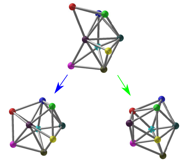
For the topology of the merging trees varies with both parameters and potential. The Morse trees are identical for short range, but not for long range (Figure 5.) The first difference occurs at , where a single cluster merges with two distinct clusters depending on the value of . The SHS cluster as well as these two continuation possibilities are shown in Figure 6. The SHS parent cluster is built from cluster 1 of by adding two extra particles, red and pink, along non-adjacent edges of the pentagon. The leftmost child cluster looks similar and can be formed by pulling the red and pink particles toward the center of mass, close enough to bond. The rightmost child cluster is quite different, containing an octahedron fragment the others do not. In addition to the red and pink particles being pulled closer together in this cluster, the dark purple particle seems to get pushed away from the center of the cluster. This child cluster is the only remaining cluster when the range becomes , and has lower energy than the leftmost child cluster. We are not sure why the sticky parameter affects the result in this way or if there is physical intuition behind it. One possibility is that slight perturbations in the potential energy caused the optimization algorithm to find a deeper minimum.
For , merging trees continue to depend on sticky parameter and potential, although the upper portions of the trees are still independent of parameters. For both potentials the trees are exactly the same for and , respectively, though the differences for , corresponding to a range of about % of particle diameter, in both cases are minimal; a difference of between to nodes.
| Morse | Lennard-Jones | Comparison | |||||||
| L-M | M-H | L-H | L-M | M-H | L-H | L | M | H | |
| 6 | 0 | 0 | 0 | 0 | 0 | 0 | 0 | 0 | 0 |
| 7 | 0 | 0 | 0 | 0 | 0 | 0 | 0.7 | 0.7 | 0.7 |
| 8 | 0 | 0 | 0 | 0 | 0 | 0 | 4.1 | 4.1 | 4.1 |
| 9 | 0.6 | 0.6 | 0.1 | 0.6 | 0.1 | 0.6 | 12 | 11 | 12 |
| 10 | 14 | 13 | 21 | 21 | 22 | 18 | 125 | 128 | 132 |
| 11 | 67 | 65 | 63 | 74 | 78 | 76 | 702 | 713 | 711 |
For these larger values of , it is hard to compare the topology of the trees quantitatively, so instead we compare the geometry of the individual clusters. Suppose we wish to compare two sets of clusters at a given range, where each set is obtained by performing continuation with different well-depth parameters or potential. There is a one-to-one mapping between the sets of clusters, because each cluster comes from a unique SHS cluster. We use this mapping to compare clusters: for each pair that comes from the same SHS cluster, we compute the root mean square deviation (RMSD; see Appendix VI.2 for details.) We then sum the RMSD over all clusters to obtain a metric comparing the sets, which we call the total RMSD. We compute the total RMSD as a function of the range parameter .
Figure 7 shows the total RMSD as a function of for , for clusters from different potentials or different (different well-depths , since the ranges at which they are compared is the same.) Remarkably, the total RMSD is nearly zero for all comparisons until relatively long ranges, roughly , or about 35% of particle diameter. This means that not only are the topologies of the merging trees nearly the same up to longer ranges, but, the geometries of the clusters themselves are also nearly the same – in other words, for a fixed range, it doesn’t matter whether you use a Morse or a Lennard-Jones potential, or what you choose for the well-depth (within the limits we considered); the metastable states are nearly identical.
For longer ranges, the total RMSD increases the most for clusters from different potentials: the geometry of the metastable states is sensitive to the choice of potential. The total RMSD increases only a little bit for clusters from the same family of potential but with different well-depths; here the clusters have a much more similar geometry. The differences could be caused by slight differences in geometry, or by merging at slightly different ranges; we cannot tell the difference using this metric. Table 2 shows a more extensive comparison than is contained in the figure, and supports the observation that there is more variety between families of potentials than within a single family.
Finally, we return to the observation that for merges at small , exactly one parent transitioned smoothly, and we ask whether this holds true for larger as well. We consider every merge event for and compute the RMSD between each cluster just before and just after it merged. For each group of merging clusters, we find exactly one cluster with a small RMSD, and all the others have much larger RMSDs (Figure 8.) Therefore, up to there is a unique smoothly-varying parent cluster for each merge event. This observation also suggests that the merges occur as fold bifurcations, in which a local maximum and local minimum annihilate, leaving no extrema. The annihilated local minimum then jumps abruptly in configuration space upon optimization past the bifurcation. The merges do not appear to occur as pitchfork bifurcations, in which two local minima separated by a local maximum smoothly coalesce into a single local minimum; such a bifurcation would give two smoothly-varying parents.
III.3 Predicting merge events




Next we ask whether there is a geometric criterion that governs when clusters merge. Intuitively, we expect that a cluster rearranges when the range of the pair potential becomes comparable to the distance between a pair of non-bonded particles.
To make this hypothesis quantitative, we define a function to be the minimum inter-particle distance that is greater than 1, for cluster at range parameter . Our hypothesis is that merges depend on in some way.
To investigate how the function behaves, we plot it as a function of in Figure 9 for two Morse clusters at , clusters and in clusters. The SHS clusters have . As decreases, decreases smoothly past , whereas jumps at , from to , when the cluster rearranges and becomes identical to cluster 9.
This behavior is the same for all merges that occur at for . In each merge, the cluster that rearranges has and the cluster that varies smoothly has . Just before the merge, the values are also the same across all merges: . Interestingly, the cluster that transitions smoothly is always the one that has the largest minimum eigenvalue in the Hessian at .
One might guess from this data that , the minimum gap in the SHS cluster, directly determines the value at which a cluster first rearranges. Unfortunately, the story is not so simple: among clusters with , there are clusters with , with values of ranging from to . To show this non-uniqueness, a scatter plot of vs. is shown in Figure 14 in Appendix VI.4.
What is true is that , the minimum distance for non-bonded particles just before the rearrangement, determines . Figure 10 shows a scatter plot of versus for all clusters that rearrange, for both potentials. The data is very well fit by the curve , which we obtained using nonlinear least squares to fit the data with a function of the form . Since the width of the attractive well of the potential scales with as , where is a constant, this fit is strong support for the hypothesis that a cluster’s first rearrangement occurs when the closest non-contacting pair comes within the range of the pair potential. The distance of this non-contacting pair can change during the continuation, which is why the distance in the SHS cluster does not determine the range at which the cluster rearranges (it does seem to determine it approximately, since the distance doesn’t usually change too much during the continuation. See Appendix VI.4.) What is useful about our formula is that it gives a specific number with which to measure the width of the potential – it tells us that when the gap between particles is closer than , their interaction starts to matter.
This formula does not hold for the smoothly-transitioning parents, which comprise about 1/3 of the clusters, and initially merge without rearranging. If we applied the formula to these clusters anyways, approximating , it would falsely predict a large (short range for rearrangement.) Some of these smoothly-transitioning parents do rearrange in later merges. We tried to find a relationship between for these clusters, and the value of at which they first rearrange discontinuously, but we could not find any relationship.
Another exception to this behavior occurs for the nonharmonic clusters, which rearrange at much shorter ranges than predicted by the formula above. Every non-harmonic SHS cluster for has , so the formula above would predict they merge via re-arrangement at ; using actual distances when they rearrange, which are closer to , gives . However, most non-harmonic clusters undergo a large rearrangement at , well before the minimum gap is within the range of the potential.
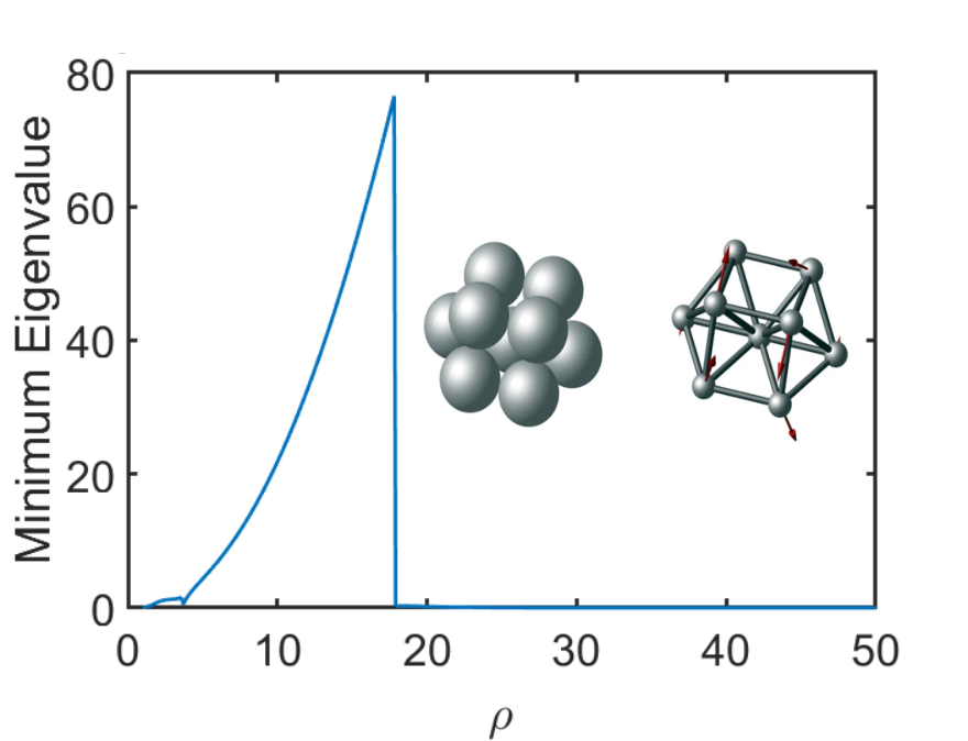
This suggests that nonharmonic clusters rearrange by a more global mechanism. To explore this mechanism, recall that nonharmonic clusters reach saddle points during the minimization for larger values of and a re-optimization procedure is performed. The result of the re-optimization is a cluster that is structurally very similar to the starting non-harmonic cluster, with a non-zero but very small minimum eigenvalue. The cluster stays close to this configuration until , when it rearranges and merges with harmonic clusters. As an example, Figure 11, which plots the minimum eigenvalue in the Hessian of the energy for the non-harmonic cluster. As decreases, the minimum eigenvalue slowly increases from until a jump occurs near , at which point the cluster merges with a harmonic cluster. Similar behavior is exhibited for all non-harmonic clusters except for 4 (of 35) non-harmonic clusters at : they are nearly constant, with a small minimum eigenvalue, until they rapidly rearrange at . The exceptions at had a minimum eigenvalue that moved away from zero before the cluster merged.
We examine the non-harmonic cluster for in detail. This cluster, as well as most others, has a planar or near planar set of particles that attach to each other in a ring and to a seventh central particle. This cluster stays nearly the same until when the particles on the outer ring begin to separate. This outer ring then begins to be pulled downward until where the cluster rearranges and merges with another cluster. Various stages of this process are shown in Figure 12. This general rearrangement mechanism occurred for most of the non-harmonic clusters.


Despite being able to often predict when a cluster will merge based on its geometry, we have not found a way to predict which clusters will merge together. One idea was to compute an adjacency matrix for each cluster representing the pairs of particles whose distances are comparable to the minimum distance between non-bonded particles, and then to compare adjacency matrices. This doesn’t work unfortunately; a counterexample is shown in Figure 13.
IV Conclusion
We used numerical continuation to study the evolution of sticky hard sphere clusters as the range of interaction increased, for Morse and Lennard-Jones potentials. This procedure finds most local minima of the smoother energy landscapes; the relatively few unmatched clusters were higher-energy clusters. This suggests that a similar technique could be used to find deep minima of larger systems, since SHS clusters with a maximal number of contacts can sometimes be found theoretically Bezdek:2012if; Bezdek:2018vt, but exploring short-range energy landscapes numerically is a challenge because the potential develops very high gradients.
As the range of interaction increased, distinct clusters merged together, so the total number of unique clusters decreased. Interestingly, we found no non-trivial splitting events, where one cluster split into two unrelated by rotations or permutations. We analyzed the mechanism behind individual merge events in details for small clusters. Many larger clusters contain these smaller clusters as sub-units, so these simple merge events provide insight into how larger clusters merge.
We found that all merges involved one cluster that varied smoothly, hence whose structure did not change, while the other clusters rearranged significantly during the merge. This suggests that all merges in our data were fold bifurcations. In addition, we found that the clusters that rearranged, did so when the range of the interaction potential became comparable to the minimum distance between particles that were not yet bonded. We found a specific formula to measure the relevant range: when the pairwise distance became about , these clusters rearranged. This formula may be useful for simulations or experiments that wish to use a threshhold distance for saying particles are bonded.
An exception to this formula occurred for the non-harmonic clusters, which rearranged by a more global mechanism.
We compared sets of clusters obtained by continuation for different potentials and different parameters, and found the corresponding clusters to be nearly identical for short and medium ranges, roughly 30% of particle diameter, but varied quite a lot for longer ranges. There was more variation when we changed the family of potentials, than when we changed parameters within the same family of potentials.
Our observations show that for short-ranged interactions, up to about % of particle diameter, the exact choice of pair potential and parameters have a negligible effect on the number of accessible ground states and the structure of local minima on the energy landscape; however, these states do differ from SHS clusters beyond a range of about % (for the values of considered.) For longer range potentials, greater than about % of particle diameter, the particular choice of interaction potential can affect the structure of these states. An intriguing extension would be to study the dynamics as the range increases, and to find a continuation procedure to study transition rates and paths between local minima or other dynamical quantities. Are they also similarly insensitive to the choice of potential?
V Acknowledgements
The authors would like to thank John Morgan for sharing data, Maria Cameron for providing code to determine point group order, and Dennis Shasha for helpful discussions. This work was supported by the United States Department of Energy under Award no. DE-SC0012296, and the Research Training Group in Modeling and Simulation funded by the National Science Foundation via grant RTG/DMS – 1646339. M. H.-C. acknowledges support from the Alfred P. Sloan Foundation.
References
- [1] D.W. Brenner. The art and science of an analytic potential. Physica Status Solidi (b), 217(1):23–40, 2000.
- [2] D. Padmavathi. Potential energy curves and material properties. Materials Sciences and Applications, 2(2):97–104, 2011.
- [3] David Wales. Energy Landscapes. Applications to Clusters, Biomolecules and Glasses. Cambridge University Press, 2003.
- [4] Vinothan N. Manoharan. Colloidal matter: Packing, geometry, and entropy. Science, 349(6251), 2015.
- [5] Massimo G. Noro and Daan Frenkel. Extended corresponding-states behavior for particles with variable range attractions. The Journal of Chemical Physics, 113(8):2941–2944, 2000.
- [6] Guangnan Meng, Natalie Arkus, Michael P. Brenner, and Vinothan N. Manoharan. The free-energy landscape of clusters of attractive hard spheres. Science, 327(5965):560–563, 2010.
- [7] Rebecca W Perry, Miranda C Holmes-Cerfon, Michael P Brenner, and Vinothan N Manoharan. Two-Dimensional Clusters of Colloidal Spheres: Ground States, Excited States, and Structural Rearrangements. Physical Review Letters, 114(22):228301–5, June 2015.
- [8] Yoav Kallus and Miranda Holmes-Cerfon. Free energy of singular sticky-sphere clusters. Phys. Rev. E, 95:022130, Feb 2017.
- [9] R. J. Baxter. Percus-yevick equation for hard spheres with surface adhesion. The Journal of Chemical Physics, 49(6):2770–2774, 1968.
- [10] Miranda Holmes-Cerfon, Steven J. Gortler, and Michael P. Brenner. A geometrical approach to computing free-energy landscapes from short-ranged potentials. Proceedings of the National Academy of Sciences, 110(1):E5–E14, 2013.
- [11] N. Arkus, V. Manoharan, and M. Brenner. Deriving finite sphere packings. SIAM Journal on Discrete Mathematics, 25(4):1860–1901, 2011.
- [12] Robert S Hoy, Jared Harwayne-Gidansky, and Corey S O’Hern. Structure of finite sphere packings via exact enumeration: Implications for colloidal crystal nucleation. Physical Review E, 85(5):051403, May 2012.
- [13] Robert S Hoy. Structure and dynamics of model colloidal clusters with short-range attractions. Physical Review E, 91(1):012303–7, January 2015.
- [14] M. Holmes-Cerfon. Enumerating rigid sphere packings. SIAM Review, 58(2):229–244, 2016.
- [15] C Patrick Royall, Stephen R Williams, Takehiro Ohtsuka, and Hajime Tanaka. Direct observation of a local structural mechanism for dynamic arrest. Nature Materials, 7(7):556–561, June 2008.
- [16] Alex Malins, Stephen R Williams, Jens Eggers, Hajime Tanaka, and C Patrick Royall. Geometric frustration in small colloidal clusters. Journal of Physics: Condensed Matter, 21(42):425103, September 2009.
- [17] David J. Wales. A microscopic basis for the global appearance of energy landscapes. Science, 293(5537):2067–2070, 2001.
- [18] Lukas Trombach, Robert S Hoy, David J. Wales, and Peter Schwerdtfeger. From sticky-hard-sphere to Lennard-Jones-type clusters. Physical review. E, 97 4-1:043309, 2018.
- [19] Lukas Trombach and Peter Schwerdtfeger. Gregory-Newton problem for kissing sticky spheres. Physical Review E, 98(3):1, September 2018.
- [20] John W. R. Morgan, Dhagash Mehta, and David J. Wales. Properties of kinetic transition networks for atomic clusters and glassy solids. Phys. Chem. Chem. Phys., 19:25498–25508, 2017.
- [21] Károly Bezdek. Contact Numbers for Congruent Sphere Packings in Euclidean 3-Space. Discrete & Computational Geometry, 48(2):298–309, February 2012.
- [22] K Bezdek and Muhammad Khan. Contact numbers for sphere packings. In Ambrus G, Bárány I, Fejes Tóth G, Pach J, and Böröczky K, editors, New Trends in Intuitive Geometry. Springer, 2018.
- [23] William H. Press, Saul A. Teukolsky, William T. Vetterling, and Brian P. Flannery. Numerical Recipes in C: The Art of Scientific Computing. Cambridge University Press, New York, NY, USA, 1992.
- [24] Davis E. King. Dlib-ml: A machine learning toolkit. Journal of Machine Learning Research, 10:1755–1758, 2009.
- [25] Anthony Trubiano. Shscontinuation. https://github.com/onehalfatsquared/SHScontinuation, 2019.
- [26] W. Kabsch. A solution for the best rotation to relate two sets of vectors. Acta Crystallographica Section A, 32(5):922–923, Sep 1976.
- [27] Mark E. Tuckerman. Statistical Mechanics: Theory and Molecular Simulation. Oxford University Press, 2010.
VI Appendix
VI.1 Optimization Algorithm
The conjugate gradient algorithm [23] was used to minimize the potential energy. For particles, the potential energy is a function of position variables. There are six degrees of freedom corresponding to rigid body translation and rotations, which are removed by constraining particle to the origin, particle to the -axis, and particle to the plane. The conjugate gradient algorithm terminates when the change in the objective function is less than and it is verified that the point is a local minimum via the eigenvalues of the Hessian. The condition number of the minimization problem scales with , so the convergence rate scales like for . However, for large enough , , so the convergence rate does not change much with sticky parameter. This is consistent with what we see in practice.
The conjugate gradient method is unstable from some starting points and can blow up or take very large steps. This depends on the value of the sticky parameter, as a larger sticky parameter corresponds to a deeper well-depth, which results in steeper gradients. A check for instability is performed after every optimization, and if either possibility occurs, we reset and try one of a variety of methods. The methods are, in order of application, gradient descent followed by conjugate gradients, conjugate gradients with resets every iterations, swapping two random particle labels among the last particles and then applying conjugate gradients, or perturbing the starting point by a random vector of norm and applying conjugate gradients. If all of these methods fail, the starting point is logged as the minimum. This usually results in a point with potential gradient norm , instead of the usual tolerance of . The fraction of optimizations that result in such an error are for .
When a saddle point is reached (minimum eigenvalue becomes negative), a re-optimization procedure is applied to reach a local minimum. This involves displacing along the eigenvector corresponding to the negative eigenvalue and re-applying conjugate gradients until a minimum is found. In some cases, a saddle point with more than one negative eigenvalue is reached; usually only , but occasionally more. We found that the choice of eigenvector to displace along did not affect the result of re-optimization, so the eigenvector corresponding to the eigenvalue of largest magnitude is chosen for consistency.
VI.2 Testing Uniqueness
To determine when two clusters are the same, we begin by checking that they have the same set of inter-particle distances. If so, the Kabsch algorithm [26] is applied to compute an optimal rotation of one cluster onto the other, and the root mean square deviation is computed as
where is the Euclidean distance between particle in cluster one and cluster two. If this is less than a tolerance of , we consider the clusters the same.
If not, we check possible permutations. To do so efficiently, we begin by computing the moment of inertia tensor, diagonalizing it, and using it to rotate each set of particles to the principal axes. Then we need to re-align (permute) the particles so both clusters have the same configuration. We do this by solving a minimum cost assignment problem, where the cost matrix is the Euclidean distance between particle in cluster one and particle in cluster two. We then re-apply the first part of the algorithm.
This still does not account for certain reflectional and rotational symmetries, so we repeat this procedure for all swaps and sign combinations of coordinates, possibilities. Taking the minimum value among all these possibilities gives the RMSD.
In the case of particles, this procedure becomes too slow to compare all pairs of clusters. In this case, we adopt a heuristic approach where we simply compare a sorted list of inter-particle distances between clusters. This is a necessary condition for uniqueness but may not be sufficient. Up to , the heuristic approach gives the same results as comparing RMSD values, so we are hopeful this extends to .
VI.3 Sticky Parameter
Here we discuss the origin of the sticky parameter, , and its relation to the second virial coefficient, . In our numerical experiments, we seek to vary the range, , of potentials, , in our continuation procedure. This leaves a free parameter in the potential function, , the well-depth. Keeping fixed as the range varies changes properties of the potential function at every stage. One such property is how “strong” a bond between two nearby particles is, which is given by the partition function
| (4) |
where is a cutoff beyond which the pair potential is essentially constant. Thus a natural way to choose after changing the range is to pick such that remains constant. To approximate this integral, we can use the method of Laplace asymptotics. The potential function has a minimum at , such that , and . We expand the potential function in a second order Taylor series to get near the minimum. The integrand then becomes a Gaussian, and since it decays very fast away from the minimum, we may extend the limits of integration to . Evaluating the Gaussian integral gives us the expression given for in the introduction,
| (5) |
We can show that our sticky parameter is related to the more commonly used second virial coefficient, . The second virial coefficient can be expressed as [27]
| (6) |
and appears as the second coefficient in a power series correction to the ideal gas law for a given interaction potential. Again, we can approximate by using Laplace asymptotics in the same way. We first note that for , . Therefore the term goes to exponentially fast, contributing nothing to the integral. Near the minimum, , and we can proceed as before. We make a second order approximation of the potential and evaluate the second moment of the Gaussian integral. The final result is
showing is a approximately linear function of the sticky parameter.
VI.4 Predicting Merge Events from SHS Geometry
We established a relationship between the value of the range parameter in which a cluster rearranges, , and the minimum distance between non-bonded particles just before this rearrangement, . Ideally, a one-to-one map between and , coming from the Sticky Hard Sphere geometry, would allow us to predict when any structure would merge. Figure 14 shows a scatter plot of vs. , with smooth transitioning clusters in blue and rearranging clusters in red. The curves are fit using non-linear least squares with the form .
Unfortunately, we find that the map is not one-to-one. There are many points for which and , but the corresponding values are spread over a large range. Despite this, does provide us with an approximation of when clusters will merge. This minimum distance can evolve differently as a function of cluster geometry, but the variations are typically small. Hence, if or , you can safely state the cluster will merge around and , respectively.
VI.5 Merging Trees


Figure 15 shows the merging tree for . As for , the tree is insensitive to the value of the sticky parameter. Changing the form of the potential affects the range at which clusters merge. Figure 16 separates the tree into the four major merge events, with SHS clusters at the top and green arrows indicating a smooth transition. In (a), we see the , mechanism is responsible for this merge. In (b), the re-arranging clusters have an octahedron as a sub-structure, and the smooth cluster is new, i.e. it does not contain any or clusters as sub-structures. In (c), all the SHS clusters have a polytetrahedron as a sub-structure, and they merge with the resulting cluster from (b). Finally (d) contains one structure with an octahedron sub-structure and a new cluster which re-arrange to form the final cluster.