Reionization optical depth determination from
Planck HFI data with ten percent accuracy
Abstract
We present an estimation of the reionization optical depth from an improved analysis of the High Frequency Instrument (HFI) data of Planck satellite. By using an improved version of the HFI map-making code, we greatly reduce the residual large scale contamination affecting the data, characterized, but not fully removed, in the Planck 2018 legacy release. This brings the dipole distortion systematic effect, contaminating the very low multipoles, below the noise level. On large scale polarization only data, we measure at C.L., reducing the Planck 2018 legacy release uncertainty by . Within the CDM model, in combination with the Planck large scale temperature likelihood, and the high- temperature and polarization likelihood, we measure at C.L. which corresponds to a mid-point reionization redshift of at C.L.. This estimation of the reionization optical depth with accuracy is the strongest constraint to date.
Key Words.
Cosmology: observations – dark ages1 Introduction
Cosmological recombination around redshift produces a mostly neutral universe, starting the so called Dark Ages. At later stages the Universe’s dark ages end with the formation of the first galaxies. The lack of Gunn-Peterson trough (Gunn & Peterson 1965; Scheuer 1965) in the spectra of distant quasars (Rauch 1998; Becker et al. 2001; Fan et al. 2006) revealed that the Universe had become almost fully reionized by redshift (Dayal & Ferrara 2018).
In the context of cosmological observations, Cosmic Microwave Background (CMB) generated at recombination and propagating almost freely to us, is mostly influenced by the total amount of free electrons along the line of sight, parametrized by the Thomson scattering optical depth to reionization , one of the six parameters of the CDM model.
Reionization has mainly two effects on CMB power spectra. Firstly, it damps by a factor scalar perturbations as generated at recombination. This makes the amplitude of the scalar perturbation highly degenerate with for high multipoles measurements. Secondly the re-scattering of the CMB photons on free electrons at the reionization epoch generates a bump on polarization power spectra at large angular scale. The position and height of this bump depend on the mean reionization redshift () and on the duration of the reionization transition. The measured quantity on the spectra at high multipoles is and thus . The measure of the large scale polarization allows to break the degeneracy with and provides directly . A ten percent relative accuracy on correspond to a accuracy on if is about . The direct measurement of on the reionzation peak is thus critical.
Although the reionization optical depth determination has been greatly improved in the last two decades, is still the less constrained parameter of the CDM model (Weiland et al. 2018; Planck Collaboration VI 2019). The reionization peak being visible only at very large scales () both in and spectra, it has been directly measured only on full sky polarized observations by space experiments. The first measurement from Wilkinson Microwave Anisotropy Probe (WMAP) (Kogut et al. 2003) gave based on spectrum, while on the final 9yr WMAP maps Hinshaw et al. 2013 reported measured on and spectra. Planck collaboration in a re-analysis of the WMAP maps (Planck Collaboration V 2019) used the Planck 353GHz map as dust tracer rather then the WMAP dust template (Page et al. 2007), based on the starlight-derived polarization directions and the Finkbeiner-Davis-Schlegel dust model (Finkbeiner et al. 1999), lowering by roughly to .
Using Planck only data and Low Frequency Instrument (hereafter LFI) 70 GHz (Planck Collaboration II 2019) map as main cosmological channel, Planck Collaboration found compatible values of in the 2015 release (Planck Collaboration XI 2016) and in the 2018 legacy release (Planck Collaboration V 2019). After the Planck 2015 release Lattanzi et al. 2017 reanalyzed all the available datasets and combined LFI 2015 data with WMAP finding .
All those results are obtained using the same general method, i.e. CMB maps are cleaned from foreground contamination and then the probability is directly computed on maps assuming Gaussian signal and noise (Tegmark 1996; Page et al. 2007; Lattanzi et al. 2017). This relies on accurate estimation of the noise bias covariance matrix. An exhaustive review of all the measures before the Planck 2018 legacy release can be found in Weiland et al. 2018.
For the Planck HFI data, being more sensitive than WMAP and LFI channels, but then more vulnerable to systematic effects, a different approach was followed by the Planck Collaboration. In this case, given the difficulty of estimating reliable covariance matrices, a spectrum based likelihood was developed, acting on the cross-spectrum of 100 and 143 GHz maps. Following this approach, Planck Collaboration Int. XLVI 2016 measured in an intermediate analysis of HFI data after the Planck 2015 release, while is reported in the Planck 2018 legacy release (Planck Collaboration V 2019).11 1 A more conservative analysis based on pseudo- estimator (Hivon et al. 2002; Tristram et al. 2005) is presented in Planck Collaboration Int. XLVII 2016 which reports . Overall, still the major limitation is the presence of large scale systematic effects, highly reduced with respect to Planck 2015 analysis but not brought below the noise level.
For a clearer global picture we report the main constraints to date, in the base CDM model, for different large scale CMB datasets:
| (1) |
the first value reported represents the final bound of WMAP Collaboration; the second is the most recent WMAP bound when the Planck 353 GHz map is used for the thermal dust cleaning; the last two values represent the Planck 2018 legacy release bounds obtained using respectively LFI and HFI.
In this paper, we present an advanced approach to the Planck HFI data in the attempt of reducing the systematic effects affecting the large scale polarization with the purpose of improving and solidifying the constraints of . We upgrade the SRoll mapmaking algorithm introduced in Planck Collaboration Int. XLVI 2016 (hereafter SRoll1) with a new cleaning of residual distortions of the large signals, we call this new algorithm SRoll2 (Delouis et al. 2019).
2 Map-making improvements
The 2018 legacy HFI maps (Planck Collaboration III 2019) represent a great step forward in the attempt of cleaning systematic effects contaminating the large scale polarization. In particular, the impact of the non-linearities of the analogue-to-digital converters (ADCs) of readout chains has been substantially reduced, introducing variation in the gain of bolometer readout chains. This correction accounts for the first-order approximation of the ADC non-linearity (ADCNL) systematic effect, but still, large signals, such as foregrounds on the Galactic plane and dipoles, are affected by the second-order ADCNL effect. This was not treated by the Planck Collaboration (see Section 5.13 of Planck Collaboration III 2019 for details), leaving large scale residuals in polarization mainly due to a mismatch that, violating the stationarity of the signal in a given pixel, causes temperature to polarization dipole leakage.
For the analysis presented in this paper, we improve the SRoll1 code in what we call SRoll2, in order to further reduce the polarization leakage due to strong signals. In the following, we list the main modifications introduced in the SRoll2 code, for more details, see Delouis et al. 2019:
- –
New ADCNL correction is obtained by fitting the residuals with a bi-dimensional spline model per bolometer as a function of signal value and time. This solution removes the apparent gain variation of bolometers allowing to fit only one gain for the entire mission. As demonstrated in Delouis et al. 2019, time variation is only necessary to capture the ADCNL at 143 GHz, and thus for the 100 and 353 GHz bolometers, only a mono-dimensional spline is considered. We verify that, for those channels, opening the time variation does not improve substantially the solution.
- –
Internal fit of (and subsequently marginalization over) the polarization angle and polarization efficiency per bolometer.
- –
Update of the CO template based on 2015 Planck release, used for the bandpass mismatch fit, introducing two new templates based on 12CO and 13CO extracted as described in Planck Collaboration III 2019 section 3.1.3 and in Delouis et al. 2019 section 4.1.
- –
Update of the thermal dust template using a map based on 2018 legacy release (for details, see section 4.1 of Delouis et al. 2019).
- –
Update of the real part of the empirical transfer function used at 353 GHz, replacing the real harmonic ranges of the spin frequency used in the Planck 2018 legacy release (see Planck Collaboration III 2019 section 2.2.2) by a single s time constant (for details see section 4.2.2 of Delouis et al. 2019).


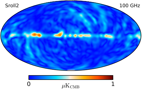

Figure 1 shows polarization intensity maps (defined as ) at 100 and 143 GHz obtained simulating realistic sky signal affected by ADCNL and projected with SRoll1 and SRoll2 codes. From those maps, we remove the input sky. In the first row, we show maps obtained with SRoll1 without gain variation. In the middle row, the maps are obtained using SRoll1 opening the gain variation and fitting 128 gain steps as done in Planck Collaboration III 2019. In the last row, the simulated timelines are projected into maps with the SRoll2 code. The large scale dipole leakage present in the first panel is substantially reduced by the introduction of gain variability (second panel) which still leaves level residuals as already shown Planck Collaboration III 2019. This residual is further reduced by SRoll2 demonstrating that the ADC-NL correction allows to fit a single gain for the bolometers as expected from pre-flight analysis (Holmes et al. 2008; Pajot et al. 2010; Catalano et al. 2010).
In Figure 2, we report the pseudo power spectra () of the residual systematic effects (hereafter systematics) maps shown in Fig. 1. The level of those residuals is pushed below both for 100 and 143 GHz by SRoll2, gaining an order of magnitude with respect to SRoll1 results. Furthermore, those residuals are weakly correlated, as can be seen in Fig. 3. In the cross-spectrum, the level of systematics is further reduced below (green line of Fig. 3). With SRoll2, systematics are negligible with respect to a typical CMB power spectrum and below the gaussian noise level 22 2 The noise spectrum shown in Fig. 3 should not be interpreted as noise level biasing the cross-spectrum estimate, by definition unbiassed, but as noise contribution entering, together with the theoretical CMB spectrum, in the error computation..
Besides, we start to be limited by the quality of the dust template, given that the level of residual systematic effects in the spectrum (green line of Fig. 3) is below or at most equal to the systematics still present in the 353 GHz channel used as dust template for both 100 and 143 GHz (purple line).
Similar improvement is easily recognizable in SRoll2 maps of data. In Figures 4 and 5, we show 100 and 143 GHz maps after the removal of diffuse Galactic foreground contamination for both SRoll1 and SRoll2. The overall level of systematics is significantly reduced everywhere in the maps by SRoll2. Both the large scale spurious structures associated to dipole leakage and the Galactic disc residuals are substantially improved.


3 Power spectrum
This section describes the power spectrum computation made using SRoll2 maps and the analysis performed on simulations. As a general approach, we follow the procedure adopted for HFI low- analysis presented in Planck Collaboration V 2019 (section 2.2). In short, 100 and 143 GHz maps, built only using polarization sensitive bolomenters (PSBs), undergo the following procedure:
- –
We filter them with a cosine window function (Benabed et al. 2009; Planck Collaboration Int. XLVI 2016), downgrading to HEALPix (Górski et al. 2005) resolution. In order to maintain the covariances invertible, we add of diagonal regularization noise.
- –
We remove the Galactic foreground contamination through template fitting. We employ SRoll2 353 GHz map for thermal dust removal and, WMAP 9yr K and Ka bands for synchrotron at 100 and 143 GHz respectively. The scalings found are reported in Tab. 1
- –
We compute the cross-QML (Planck Collaboration V 2019; Tegmark 1996; Tegmark & de Oliveira-Costa 2001; Efstathiou 2006) power spectrum between 100 and 143 GHz cleaned maps (see Fig. 7) outside a Galactic mask (see Fig. 6). As temperature map, we use the Planck 2018 Commander solution (Planck Collaboration IV 2019; Planck Collaboration V 2019) smoothed with a 440 ′(7.3 ∘) gaussian beam and regularized with diagonal noise. As covariance matrices, we use FFP8 covariances (Planck Collaboration VIII 2016; Planck Collaboration XII 2016) for the HFI channels, and for WMAP K and Ka, the official 9yr matrices (Bennett et al. 2013).
|
The same cleaning procedure is applied to a set of 500 Monte Carlo simulations containing realistic sky signal, noise and systematic effects. The fiducial CMB map contained in those simulations is removed after the foreground cleaning leaving only maps with noise, systematic effects and foreground residuals, referred hereafter as N+S+F-MC (for Noise, Systematics and Foreground residuals Montecarlo) .
As already stated in Planck Collaboration Int. XLVI 2016 and Planck Collaboration V 2019, FFP8 covariance matrices (Planck Collaboration XII 2016) represent a sub-optimal, but unavoidable, choice. The FFP8 covariance matrices are built following the method presented in Keskitalo et al. 2010 (see in particular section 3.2). They are assembled in two pieces, one describing the sub-baseline correlation part which is untouched by the destriper mapmaking and one describing the ring-to-ring correlation due to errors in solving for the baselines. Consequently those matrices do not capture properly the variance of the systematic effects but only the white and noise components, assuming an analytical model for the noise spectrum33 3 FFP8 covariance matrices can be obtained upon specific request to the Planck Project Scientist at ESTEC or directly to NERSC.. Despite that, since we rely on cross-spectrum estimator, this choice does not impact power spectrum estimate but only its optimality (see e.g. Planck Collaboration Int. XLVI 2016; Planck Collaboration V 2019).
Furthermore, for SRoll2 maps, having the residual systematics further reduced with respect to noise (see Fig. 3), we have a more efficient estimator than the analysis performed for Planck 2018 legacy release.
All masks used for foreground cleaning (see Fig. 6), power spectrum estimation and likelihood are obtained thresholding the sum of dust polarization intensity scaled at 143 GHz with synchrotron polarization intensity scaled at 100 GHz, both smoothed with a Gaussian window function with full with half maximum of 7.5 ∘. As dust and synchrotron tracers, we use Planck 353 GHz, scaled by and WMAP K band, scaled by . The mask used for the foreground template fitting, both for data and simulations, retains 70 % of the sky. The other masks are used in the cosmological analysis.

Figure 7 shows the power spectrum of the SRoll2 maps compared with the Planck 2018 power spectrum both on % of the sky. The error bars are obtained combining a Monte Carlo of CMB signal with with N+S+F-MC, and computing the QML power spectrum from all the maps. The quadrupole affecting Planck 2018 analysis is radically reduced by the new map-making procedure.
In Fig. 8, we compare the error bars purged from cosmic variance obtained in SRoll2 maps with the ones of Planck 2018 analysis. With the SRoll2 maps, we manage to halve quadrupole and octupole errors with respect to the Planck 2018 analysis. Overall the entire range of multipoles sensitive to reionization optical depth shows a clearly reduced level of residual systematic effects and a lower variance. Furthermore, the s are weakly correlated as shown in Fig. 9. In the range relevant for estimation , the multipoles are substantially uncorrelated, with the scatter observed in the off-diagonal correlation perfectly compatible with the number of N+S+F-MC simulations. In the region where the signal is expected to be very small in CDM model () we notice the presence of a weak (up to ) correlation, nevertheless this feature is not expected to affect substantially the estimation.
By comparing the fraction of the error due to noise and systematic effects with the cosmic variance for , in the range , we notice that, for the first time, we start being dominated by the latter, as shown in Fig.10. All the error bars are obtained using simulations and not computed analytically.
In Fig. 11, we compare power spectrum obtained with different masks. The multipole shows the largest variation throughout the various masks. We verify, using simulations, that this variation is always consistent with fluctuation. We emphasize again that N+S+F-MC contains noise, systematic effects and residuals of foreground cleaning.
As final test, we show in Fig. 12 the power spectrum obtained from the cross-correlation of 100 and 143 GHz SRoll2 maps. As reference, we jointly plot Planck 2018 legacy release power spectrum (Planck Collaboration V 2019). Both spectra are compatible with null signal, with SRoll2 being more constraining at very large scale. The probability to exceed is PTE=0.73, for Planck 2018, and PTE=0.86, for SRoll2. The large negative quadrupole in Planck 2018 legacy release, related to ADCNL residuals (see Planck Collaboration III 2019 and Planck Collaboration V 2019), is almost completely reabsorbed in the new analysis. As final test, assuming the empirical distribution of the N+S+F-MC simulations and the power spectra measured on data computed on the 50% mask, in Tab. 2 we report, -by-, the percentage of simulations that have an absolute value of the difference between and the barycenter of the distribution larger than the same quantity measured on data. Also in this case, the overall agreement is excellent, with no particular outliers.
|
4 Likelihood and estimation
Following the procedure presented in Planck Collaboration V 2019, we build a likelihood for , based on power spectrum in the multipole range . In details:
- –
we generate 101 theoretical power spectra, , equally spaced in the range , varying accordingly such that as in Planck Collaboration Int. XLVI 2016. The other CDM cosmological parameters () are fixed to the best fit model of Planck Collaboration VI 2019;
- –
for each , we build a CMB signal Monte Carlo of 500 maps;
- –
we combine N+S+F-MC with the signal Monte Carlo, and we compute the spectrum for each realization. We compute the power spectrum also for data, ;
- –
histogramming the simulations -by- and -by-, we build empirically the probability ;
- –
with a piecewise polynomial function we interpolate in order to smooth the scatter due to limited number of simulations available;
- –
assuming negligible correlation between multipoles (see Fig. 9), we compute the probability for each value in our grid:
(2)
With this algorithm, we can draw slices of probability for adopting different sky fractions and multipole ranges, in order to stress the stability of the analysis and to perform consistency tests.
As a first consistency check, we test how the sky fraction used to compute the power spectrum impacts the constraint. We explore the same masks used in Fig. 11 and shown in Fig 6. In Fig. 13, we show a whisker plot with best-fit values, 68% and 95% confidence levels on for spectra computed with different QML masks, ranging from 20 to 60% of used sky. The posteriors are stable, all within one . We verify on simulations the statistical consistency of the values computed on different masks, finding a consistency always better than throughout the various masks, having accounted for the common sky, noise and systematics. As baseline, we adopt the mask where we measure a reionization optical depth of:
| (3) |
having fixed .
In the following part of this section, we show tests performed only on the sky mask.
Figure 14 shows the effect of changing the minimum multipole used in Eq. 2. The posteriors are stable up to , further explorations being less meaningful due to the drop of the reionization feature above those multipoles.
In Fig. 15, we test the stability of posterior when one multipole at a time is removed from the summation in Eq. 2. The maximum variation is observed when is removed causing a roughly half- shift in the posterior. This shift was consistently observed by analogous analysis performed on previous versions of the same HFI data (see e.g. Planck Collaboration Int. XLVI 2016 figure D.9 and Planck Collaboration V 2019 figure 14) with SRoll2 being less discrepant despite the smaller overall error budget. Also in this case, we verify on simulations that the obtained removing is consistent with a statistical fluctuation when compared with the one obtained using the full range.
We also explore the stability of the constraint changing the synchrotron tracers used respectively for 100 and 143 GHz. In figure 16 we show posteriors obtained using different combinations of the available synchrotron tracers, WMAP K band, WMAP Ka band or LFI 30 GHz (Planck Collaboration II 2019), all the posteriors are extremely consistent demonstrating that the synchrotron subtraction does not represent a critical point, as already discussed in Planck Collaboration V 2019.
We tested the quality of the dust removal employing the 217 GHz instead of 353 GHz for the cleaning of 100 GHz. In figure 17 we compare the posterior obtained cleaning both 100 and 143 GHz using 353 GHz with the one obtained by cleaning 100 GHz with 217 GHz and 143 GHz with 353 GHz. The consistency is remarkable, with only the latter showing slightly larger error bars, likely due to the smaller leverage of 217 GHz not fully compensated by the lower noise.
Finally, we attempt a similar analysis on the spectrum only, measuring for the same 50% mask, finding:
| (4) |
which nicely confirms the based result. It is worth to mention here that the poor PTEs for the null TE spectra found in the Planck 2018 likelihood analysis (Planck Collaboration V 2019) are still present in this version of the data, even if with slightly less significance. We recall also that we employ the same Commander solution used in the Planck 2018 likelihood, thus based on SRoll1 maps.
5 Impact on cosmology
Following the method presented in Planck Collaboration V 2019 and used for the Planck SimAll likelihood (i.e. lowE in Planck 2018 legacy release) we build a likelihood for SRoll2 100x143 power spectrum44 4 For details about validation and performances of the likelihood approximation see Gerbino et al. 2019.. We call this new likelihood module lowE-S2 55 5 The likelihood module is built within the clik infrastructure (Planck Collaboration XV 2014; Planck Collaboration ES 2013; Planck Collaboration ES 2015; Planck Collaboration ES 2018) and it is available on http://sroll20.ias.u-psud.fr or on https://web.fe.infn.it/pagano/low_ell_datasets/sroll2 .
Superseeding the Planck lowE likelihood, we combine the lowE-S2 with the high- Plik 2018 likelihood and with the Commander 2018 low- temperature likelihood in order to constrain cosmological parameters. In this section, we explore the cosmological parameter space making use of the cosmomc66 6 http://cosmologist.info/cosmomc package (Lewis & Bridle 2002) based on camb77 7 http://camb.info Boltzmann code (Lewis et al. 2000). The global settings in terms of parametrization and assumptions are coherent with Planck Collaboration VI 2019.
First of all, we combine lowE-S2 with only with Commander 2018 temperature likelihood, and we estimate the cosmological parameters only sampling and , keeping fixed the other parameters to Planck TT+lowE bestfits, measuring
| (5) |
which is directly comparable with the bounds shown in Eq. 1. The amplitude of the scalar perturbations preferred by the temperature likelihood is substantially low (see e.g. Planck Collaboration V 2019 Table 4 and 12) which is compensated by an increase of the value. Opening the other CDM parameters, and adding the TT likelihood drives the value of upwards
| (6) |
Similar behaviour was also observed in Planck Collaboration VI 2019 and Planck Collaboration XIII 2016 and is mainly due to the degeneracy broken by the high- lensing in the temperature spectrum. The addition of high- polarization drives again upward and thus the optical depth up to:
| (7) |
The fluctuation amplitude can be directly constrained at late times by CMB lensing reconstruction power spectrum (Planck Collaboration VIII 2019), partially degenerated with the matter density, while the BAO measurements constrain very efficiently the geometry of the late universe (see Planck Collaboration VI 2019 for more details on those datasets). Nonetheless the combination of Planck 2018 lensing likelihood and BAO measurements with the primary CMB anisotropies does not improve significantly the constraint:
| (8) |
Assuming a parametrization of the ionization fraction, the constrain can be translated into a mid-point redshift of reionization of:
| (9) |
consistent with the latest astrophysical constraint of high-redshift quasars (see e.g. Becker et al. 2001, Fan et al. 2006 and Bouwens et al. 2015 for an exhaustive comparison).
The combination of low and high- likelihoods breaks efficiently the degeneracy, giving:
| (10) |
In the context of CDM model, this bound can be directly translated in the parameter
| (11) |
which measures the amplitude of the matter power spectrum on the scale of .
Bounds on the CDM native parameters and some meaningful derived ones are reported in Tab. 3 where we compare the results obtained with the Planck 2018 baseline likelihood with the ones obtained replacing lowE with lowE-S2.
|
We also consider minimal one parameter extensions of the CDM model such as , , and finding no relevant changes with respect to the Planck 2018 legacy release bounds (Planck Collaboration VI 2019) which reinforce the overall stability of the Planck 2018 results. This is likely to be connected to the mostly unchanged upper limit on , i.e. at 95% C. L..
Finally, we explore the phenomenological parameter which rescales the lensing potential with respect to the theoretical expectation within CDM model. Consistently throughout Planck releases the CMB power spectra show a preference for (Planck Collaboration XVI 2014; Planck Collaboration XIII 2016; Planck Collaboration VI 2019), see Planck Collaboration Int. LI 2017 for extensive discussion. Such values of are in slight tension with the theoretical expectations and with the ones extracted from the lensing reconstruction power spectrum (Planck Collaboration VIII 2019). Combining temperature and polarization data, in the Planck 2018 legacy release, was measured. Replacing lowE with lowE-S2 slightly reduces the lensing amplitude down to , without changing the overall conclusions of Planck Collaboration VI 2019. This is again explainable with the increase of connected with the increase of which allows a slightly lower lensing amplitude.
6 Conclusions
In this paper we present an improved constraint on the reionization optical depth , obtained analyzing the Planck HFI data with an updated version of the SRoll map-making algorithm called SRoll2 specifically designed to reduce the residual large scale polarization systematics still present in the Planck HFI 2018 legacy maps. Details and performances of the SRoll2 algorithm are described extensively in Delouis et al. 2019.
The level of residual systematics associated to the first multipoles, relevant for estimation, is brought below the noise level and for the first time the cosmic variance becomes the main source of uncertainty in CMB large scale polarization parameter estimation.
As explained in Planck Collaboration V 2019 (see in particular section 2.4) the level of T to P leakage in the Planck 2018 legacy release maps forced the Planck Collaboration to adopt a strategy for the large scale polarization likelihood entirely based on simulations. Furthermore the difficulty of building reliable covariance matrices leads to use a simulation based likelihood, built on the cross spectrum of 100 and 143 GHz. In the present analysis, we follow the same overall strategy, although the lower level of systematics could have allowed a semi-analytical approach (see e.g. Mangilli et al. 2015; Vanneste et al. 2018; Hamimeche & Lewis 2008; Gerbino et al. 2019) which we leave to future analysis. With this method, we measure at C.L. when all the other CDM parameter are kept fixed.
The main difference with respect to the Planck 2018 analysis (which yields ) is based on the correction of the second-order ADCNL effect presented in Delouis et al. 2019 which drastically reduces the dipole and foreground signals distortion allowing to recover almost completely and for the determination, suppressed in previous analysis by a large variance (see e.g. Planck Collaboration Int. XLVI 2016; Planck Collaboration V 2019; Planck Collaboration Int. XLVII 2016). As consequence of this in the SRoll2 100x143 spectrum the variance associated to systematics becomes smaller than the noise and cosmic variance making less critical the accuracy of the ADCNL simulation produced. Those aspects together with an improved version of the foreground model causes a 1- upward shift in the posterior.
In a more complete parameter exploration, combining the SRoll2 likelihood with the temperature and high- polarization likelihood, we measure at C.L. which represents the strongest constrain on the reionization optical depth to date. The most recent optical depth measurement from CMB data in the context of CDM model are reported in Fig. 18.
Assuming instantaneous reionization, this corresponds to at C.L. The tight bound on breaks efficiently the degeneracy reducing the constraint on the fluctuation amplitude down to at C.L..
The improvement with respect to Planck 2018 legacy release in the large scale polarization data leads to an expected reduction of the uncertainty but it is matched with a slight shift upwards of the central value. This combination leads to a substantial unchanged upper limit leaving to a mostly unchanged constraint on all the minimal CDM extensions explored. Further investigations are left to future publications. The SRoll2 data maps, simulations and, likelihood code are publicly available at http://sroll20.ias.u-psud.fr.
Acknowledgements.
We acknowledge the use of CAMB, HEALPix and Healpy software packages. This work is part of the Bware project, partially supported by CNES. It was granted access to the HPC resources of CINES (http://www.cines.fr) under the allocation 2017-A0030410267 made by GENCI (http://www.genci.fr). This research used resources of the National Energy Research Scientific Computing Center (NERSC), a U.S. Department of Energy Office of Science User Facility operated under Contract No. DE-AC02-05CH11231. LP is grateful to G. Fabbian, M. Lattanzi and M. Migliaccio for many helpful discussions during the preparation of this work. LP acknowledges the support of the National Centre for Space Studies (CNES) postdoctoral program and Italian Space Agency (ASI) grant 2016-24-H.0 (COSMOS).References
- Becker et al. (2001) Becker, R. H. et al., Evidence for Reionization at Z 6: Detection of a Gunn-Peterson trough in a Z = 6.28 Quasar. 2001, Astron. J., 122, 2850, astro-ph/0108097
- Benabed et al. (2009) Benabed, K., Cardoso, J. F., Prunet, S., & Hivon, E., TEASING: a fast and accurate approximation for the low multipole likelihood of the Cosmic Microwave Background temperature. 2009, Mon. Not. Roy. Astron. Soc., 400, 219, 0901.4537
- Bennett et al. (2013) Bennett, C. L., Larson, D., Weiland, J. L., et al., Nine-year Wilkinson Microwave Anisotropy Probe (WMAP) Observations: Final Maps and Results. 2013, ApJ Supp., 208, 20, 1212.5225
- Bouwens et al. (2015) Bouwens, R. J., Illingworth, G. D., Oesch, P. A., et al., Reionization after Planck: The Derived Growth of the Cosmic Ionizing Emissivity now matches the Growth of the Galaxy UV Luminosity Density. 2015, Astrophys. J., 811, 140, 1503.08228
- Catalano et al. (2010) Catalano, A., Coulais, A., & Lamarre, J.-M., Analytical approach to optimizing alternating current biasing of bolometers. 2010, Appl. Opt., 49, 5938
- Dayal & Ferrara (2018) Dayal, P. & Ferrara, A., Early galaxy formation and its large-scale effects. 2018, Phys. Rept., 780-782, 1, 1809.09136
- Delouis et al. (2019) Delouis, J. M., Pagano, L., Mottet, S., Puget, J. L., & Vibert, L., SRoll2: an improved mapmaking approach to reduce large-scale systematic effects in the Planck High Frequency Instrument legacy maps. 2019, Astron. Astrophys., 629, A38, 1901.11386
- Efstathiou (2006) Efstathiou, G., Hybrid estimation of cosmic microwave background polarization power spectra. 2006, MNRAS, 370, 343, astro-ph/0601107
- Fan et al. (2006) Fan, X.-H., Strauss, M. A., Becker, R. H., et al., Constraining the evolution of the ionizing background and the epoch of reionization with z 6 quasars. 2. a sample of 19 quasars. 2006, Astron. J., 132, 117, astro-ph/0512082
- Finkbeiner et al. (1999) Finkbeiner, D. P., Davis, M., & Schlegel, D. J., Extrapolation of galactic dust emission at 100 microns to CMBR frequencies using FIRAS. 1999, Astrophys. J., 524, 867, astro-ph/9905128
- Gerbino et al. (2019) Gerbino, M., Lattanzi, M., Migliaccio, M., et al., Likelihood methods for CMB experiments. 2019, 1909.09375
- Górski et al. (2005) Górski, K. M., Hivon, E., Banday, A. J., et al., HEALPix: A Framework for High-Resolution Discretization and Fast Analysis of Data Distributed on the Sphere. 2005, ApJ, 622, 759, astro-ph/0409513
- Gunn & Peterson (1965) Gunn, J. E. & Peterson, B. A., On the Density of Neutral Hydrogen in Intergalactic Space. 1965, Astrophys. J., 142, 1633
- Hamimeche & Lewis (2008) Hamimeche, S. & Lewis, A., Likelihood Analysis of CMB Temperature and Polarization Power Spectra. 2008, Phys. Rev., D77, 103013, 0801.0554
- Hinshaw et al. (2013) Hinshaw, G., Larson, D., Komatsu, E., et al., Nine-year Wilkinson Microwave Anisotropy Probe (WMAP) Observations: Cosmological Parameter Results. 2013, ApJ Supp., 208, 19, 1212.5226
- Hivon et al. (2002) Hivon, E., Gorski, K. M., Netterfield, C. B., et al., Master of the cosmic microwave background anisotropy power spectrum: a fast method for statistical analysis of large and complex cosmic microwave background data sets. 2002, Astrophys. J., 567, 2, astro-ph/0105302
- Holmes et al. (2008) Holmes, W. A., Bock, J. J., Crill, B. P., et al., Initial test results on bolometers for the Planck high frequency instrument. 2008, Appl. Opt., 47, 5996
- Keskitalo et al. (2010) Keskitalo, R., Ashdown, M. A. J., Cabella, P., et al., Residual noise covariance for Planck low-resolution data analysis. 2010, A&A, 522, A94, 0906.0175
- Kogut et al. (2003) Kogut, A., Spergel, D. N., Barnes, C., et al., First-Year Wilkinson Microwave Anisotropy Probe (WMAP) Observations: Temperature-Polarization Correlation. 2003, ApJ Supp., 148, 161, astro-ph/0302213
- Lattanzi et al. (2017) Lattanzi, M., Burigana, C., Gerbino, M., et al., On the impact of large angle CMB polarization data on cosmological parameters. 2017, JCAP, 1702, 041, 1611.01123
- Lewis & Bridle (2002) Lewis, A. & Bridle, S., Cosmological parameters from CMB and other data: A Monte Carlo approach. 2002, Phys. Rev. D, 66, 103511, astro-ph/0205436
- Lewis et al. (2000) Lewis, A., Challinor, A., & Lasenby, A., Efficient computation of CMB anisotropies in closed FRW models. 2000, ApJ, 538, 473, astro-ph/9911177
- Mangilli et al. (2015) Mangilli, A., Plaszczynski, S., & Tristram, M., Large-scale cosmic microwave background temperature and polarization cross-spectra likelihoods. 2015, Mon. Not. Roy. Astron. Soc., 453, 3174, 1503.01347
- Page et al. (2007) Page, L., Hinshaw, G., Komatsu, E., et al., Three-Year Wilkinson Microwave Anisotropy Probe (WMAP) Observations: Polarization Analysis. 2007, ApJ Supp., 170, 335, astro-ph/0603450
- Pajot et al. (2010) Pajot, F., Ade, P. A. R., Beney, J., et al., Planck pre-launch status: HFI ground calibration. 2010, A&A, 520, A10
- Planck Collaboration ES (2013) Planck Collaboration ES. 2013, The Explanatory Supplement to the Planck 2013 results, https://www.cosmos.esa.int/web/planck/pla (ESA)
- Planck Collaboration ES (2015) Planck Collaboration ES. 2015, The Explanatory Supplement to the Planck 2015 results, https://www.cosmos.esa.int/web/planck/pla (ESA)
- Planck Collaboration ES (2018) Planck Collaboration ES. 2018, The Legacy Explanatory Supplement, https://www.cosmos.esa.int/web/planck/pla (ESA)
- Planck Collaboration XV (2014) Planck Collaboration XV, Planck 2013 results. XV. CMB power spectra and likelihood. 2014, A&A, 571, A15, 1303.5075
- Planck Collaboration XVI (2014) Planck Collaboration XVI, Planck 2013 results. XVI. Cosmological parameters. 2014, A&A, 571, A16, 1303.5076
- Planck Collaboration VIII (2016) Planck Collaboration VIII, Planck 2015 results. VIII. High Frequency Instrument data processing: Calibration and maps. 2016, A&A, 594, A8, 1502.01587
- Planck Collaboration XI (2016) Planck Collaboration XI, Planck 2015 results. XI. CMB power spectra, likelihoods, and robustness of parameters. 2016, A&A, 594, A11, 1507.02704
- Planck Collaboration XII (2016) Planck Collaboration XII, Planck 2015 results. XII. Full Focal Plane simulations. 2016, A&A, 594, A12, 1509.06348
- Planck Collaboration XIII (2016) Planck Collaboration XIII, Planck 2015 results. XIII. Cosmological parameters. 2016, A&A, 594, A13, 1502.01589
- Planck Collaboration II (2019) Planck Collaboration II, Planck 2018 results. II. Low Frequency Instrument data processing. 2019, A&A, in press, 1807.06206
- Planck Collaboration III (2019) Planck Collaboration III, Planck 2018 results. III. High Frequency Instrument data processing. 2019, A&A, in press, 1807.06207
- Planck Collaboration IV (2019) Planck Collaboration IV, Planck 2018 results. IV. Diffuse component separation. 2019, A&A, in press, 1807.06208
- Planck Collaboration V (2019) Planck Collaboration V, Planck 2018 results. V. Power spectra and likelihoods. 2019, A&A, submitted, 1907.12875
- Planck Collaboration VI (2019) Planck Collaboration VI, Planck 2018 results. VI. Cosmological parameters. 2019, A&A, submitted, 1807.06209
- Planck Collaboration VIII (2019) Planck Collaboration VIII, Planck 2018 results. VIII. Gravitational lensing. 2019, A&A, in press, 1807.06210
- Planck Collaboration Int. XLVI (2016) Planck Collaboration Int. XLVI, Planck intermediate results. XLVI. Reduction of large-scale systematic effects in HFI polarization maps and estimation of the reionization optical depth. 2016, A&A, 596, A107, 1605.02985
- Planck Collaboration Int. XLVII (2016) Planck Collaboration Int. XLVII, Planck intermediate results. XLVII. Constraints on reionization history. 2016, A&A, 596, A108, 1605.03507
- Planck Collaboration Int. LI (2017) Planck Collaboration Int. LI, Planck intermediate results. LI. Features in the cosmic microwave background temperature power spectrum and shifts in cosmological parameters. 2017, A&A, 607, A95, 1608.02487
- Rauch (1998) Rauch, M., The lyman alpha forest in the spectra of quasistellar objects. 1998, Ann. Rev. Astron. Astrophys., 36, 267, astro-ph/9806286
- Scheuer (1965) Scheuer, P. A. G., A Sensitive Test for the Presence of Atomic Hydrogen in Intergalactic Space. 1965, Nature, 207, 963
- Tegmark (1996) Tegmark, M., A method for extracting maximum resolution power spectra from microwave sky maps. 1996, MNRAS, 280, 299, astro-ph/9412064
- Tegmark & de Oliveira-Costa (2001) Tegmark, M. & de Oliveira-Costa, A., How to measure CMB polarization power spectra without losing information. 2001, Phys. Rev., D64, 063001, astro-ph/0012120
- Tristram et al. (2005) Tristram, M., Macias-Perez, J. F., Renault, C., & Santos, D., Xspect, estimation of the angular power spectrum by computing cross power spectra. 2005, Mon. Not. Roy. Astron. Soc., 358, 833, astro-ph/0405575
- Vanneste et al. (2018) Vanneste, S., Henrot-Versillé, S., Louis, T., & Tristram, M., Quadratic estimator for CMB cross-correlation. 2018, Phys. Rev., D98, 103526, 1807.02484
- Weiland et al. (2018) Weiland, J. L., Osumi, K., Addison, G. E., et al., Effect of Template Uncertainties on the WMAP and Planck Measures of the Optical Depth Due To Reionization. 2018, Astrophys. J., 863, 161, 1801.01226