From cold to hot irradiated gaseous exoplanets: Fingerprints of chemical disequilibrium in atmospheric spectrapetitCODE (Mollière et al. 2015; Mollière et al. 2017), ODEPACK (Hindmarsh 1983), and ChemKM (this work).

Karan Molaverdikhani Affiliation: Max Planck Institute for Astronomy, Königstuhl 17, 69117 Heidelberg, Germany Corresponding author: Karan Molaverdikhani Thomas Henning Affiliation: Max Planck Institute for Astronomy, Königstuhl 17, 69117 Heidelberg, Germany Paul Mollière Affiliation: Sterrewacht Leiden, Huygens Laboratory, Niels Bohrweg 2, 2333 CA Leiden, The Netherlands

Received TBD; Revised TBD; Accepted TBD

Abstract

Almost all planetary atmospheres are affected by disequilibrium chemical processes. In this paper we introduce our recently developed Chemical Kinetic Model (ChemKM). We show that the results of our HD 189733b model are in good agreement with previously published results, except at $\mu$ bar regime, where molecular diffusion and photochemistry are the dominant processes. We thus recommend careful consideration of these processes when abundances at the top of the atmosphere are desired. We also propose a new metric for a quantitative measure of quenching levels. By applying this metric, we find that quenching pressure decreases with the effective temperature of planets, but it also varies significantly with other atmospheric parameters such as [Fe/H], log(g), and C/O. In addition, we find that the “Methane Valley”, a region between 800 and 1500 K where above a certain C/O threshold value a greater chance of $\text{CH}{\vphantom{\text{X}}}_{\smash[t]{\text{4}}}$ detection is expected, still exists after including the vertical mixing. The first robust $\text{CH}{\vphantom{\text{X}}}_{\smash[t]{\text{4}}}$ detection on an irradiated planet (HD 102195b) places this object within this region; supporting our prediction. We also investigate the detectability of disequilibrium spectral fingerprints by JWST, and suggest focusing on the targets with T_eff between 1000 and 1800 K, orbiting around M-dwarfs, having low surface gravity but high metallicity and a C/O ratio value around unity. Finally, constructing Spitzer color-maps suggests that the main two color-populations are largely insensitive to the vertical mixing. Therefore any deviation of observational points from these populations are likely due to the presence of clouds and not disequilibrium processes. However, some cold planets (T_eff $<$ 900 K) with very low C/O ratios ( $<$ 0.25) show significant deviations; making these planets interesting cases for further investigation.

Keywords:

planets and satellites: atmospheres — planets and satellites: composition — methods: numerical

I Introduction

The atmospheric composition of solar system planets is not at their thermochemical equilibrium state, mostly due to the irradiation by the Sun and mixing through atmospheric transport and turbulence. These effects are so pronounced that even the earliest atmospheric models of these objects include disequilibrium chemistry (e.g. review articles on the early modern models of Venus (Noll & McElroy 1972), Earth (Lou 1973), Mars (Noll & McElroy 1974), Jupiter (Danielson 1968), Saturn (Divine 1972), Titan (Divine 1974), Uranus, and Neptune (Encrenaz 1974)).

With the discovery of Hot Jupiters (Mayor & Queloz 1995), however, the assumption of thermochemical equilibrium resurfaced as a first-order estimation of their atmospheric properties thanks to their high temperatures (Burrows & Sharp 1999; Lodders & Fegley 2002; Fortney et al. 2005, e.g.). But further studies suggested that the non-thermal processes could potentially alter their chemical composition at the photospheric levels; predominantly because of the intense UV irradiation and strong atmospheric mixing (Seager et al. 2005; Madhusudhan & Seager 2009; Stevenson et al. 2010; Moses et al. 2011; Agúndez et al. 2012; Venot et al. 2012; Hu et al. 2012; Hu et al. 2013; Hébrard et al. 2013; Hu & Seager 2014; Miguel et al. 2014; Zahnle & Marley 2014; Drummond et al. 2016; Tsai et al. 2017; Wang et al. 2017; Blumenthal et al. 2018; Zhang & Showman 2018; Changeat et al. 2019, e.g.) or other processes such as lightning (Helling & Rimmer 2019) and cosmic rays (Rimmer & Helling 2013).

Madhusudhan & Seager 2011 performed an extensive retrieval analysis of the GJ 436b spectrum observed by Stevenson et al. 2010 and concluded that the methane abundance paucity cannot be explained by thermoequilibrium chemistry. While the lack of a robust methane detection in the spectra of irradiated gaseous planets (Brogi et al. 2016; Brogi et al. 2018; Pino et al. 2018; Alonso-Floriano et al. 2019, e.g.) could be an indication of disequilibrium chemistry, there is no large-scale systematic investigation of how disequilibrium processes change the abundance of methane (or any other major opacity compound) at photospheric pressures ( $\sim$ 1 bar to $\sim$ 1 $\mu$ bar), and how this manifests itself in the atmospheric spectra. Zahnle & Marley 2014 and Miguel & Kaltenegger 2014 both perform such studies however over a limited parameter space. The complexity of photochemical models makes the large-scale simulations computationally expensive, and thus such investigations require code optimization. In addition, the models must be flexible and generic enough to perform efficiently over a range of atmospheric conditions and compositions.

We introduce a new chemical kinetic model (ChemKM), which is both fast and generic. We employ ChemKM to perform an extensive parameter study over a broad range of atmospheric conditions. In total, we calculate 84,672 full-network chemical kinetic models with more than 100 reactants and 1000 reactions, to study how the variation of major opacity sources (e.g. $\text{H}{\vphantom{\text{X}}}_{\smash[t]{\text{2}}}\text{O}$ , $\text{CH}{\vphantom{\text{X}}}_{\smash[t]{\text{4}}}$ , CO, and $\text{CO}{\vphantom{\text{X}}}_{\smash[t]{\text{2}}}$ ) due to disequilibrium chemistry affect the spectra. We also present a case study of HD 189733b, a well-studied exoplanet, for benchmarking.

In what follows, we describe our chemical kinetic model and the parameter space that we have explored. In Section III.1, we present the results of our case study for HD 189733b and benchmark it against the model developed by Venot 2012. In the rest of Section III, we present the results of our parametric study and check the validity of our proposed classification scheme for irradiated planetary spectra (see Molaverdikhani et al. 2019 for more details on the classification under cloud-free equilibrium chemistry conditions). In Section III.3, we report the dependency of quenching point on atmospheric parameters, and in Section III.4 we investigate the detectability of disequilibrium processes by JWST. Finally, in Section III.5 we discuss Spitzer transmission and emission color diagrams variation from thermochemical equilibrium models due to the vertical mixing, and its observability. We summarize and conclude our results and findings in Section IV.

II Methods

II.1 ChemKM: The Chemical Kinetic Model

To study the effects of disequilibrium chemistry on the composition and atmospheric spectra of irradiated exoplanets we developed a 1D Chemical Kinetic Model (ChemKM). The abundances of atmospheric constituents are governed by numerically solving the equations of chemical kinetics (also known as the altitude-dependent continuity–diffusion equation) which describe the formation and destruction of species, equation 1 (Allen et al. 1981, e.g.):

\frac{\partial n_{i}}{\partial t}=P_{i}-L_{i}-\frac{\partial\Phi_{i}}{\partial z},

(1)

where $n_{i}$ is the number density (cm^-3), $P_{i}$ is the chemical production rate (cm^-3 s^-1), $L_{i}$ is the chemical loss rate (cm^-3 s^-1), and $\Phi_{i}$ is the net vertical flux (cm^-2 s^-1) of species $i$ at altitude z. These quantities are all functions of time $t$ and altitude $z$ (or alternatively pressure). The vertical flux transport terms include molecular and eddy diffusion, $\Phi_{i}$ = $\Phi_{i,mol}$ + $\Phi_{i,eddy}$ where the latter is commonly parameterized by an eddy diffusion coefficient K_zz. The vertical flux transport terms can be estimated through equations 2 and 3, respectively (see e.g. Moses 1991 and references therein).

\Phi_{i,mol}=-n_{T}D_{i}\Big(\frac{\partial f_{i}}{\partial z}-\frac{f_{i}}{H_{a}}+\frac{f_{i}}{H_{i}}+\frac{\alpha_{i}f_{i}}{T}\frac{dT}{dz}\Big)

(2)

\Phi_{i,eddy}=-n_{T}K_{zz}\Big(\frac{\partial f_{i}}{\partial z}\Big),

(3)

where K_zz is the eddy diffusion coefficient (cm² s^-1), $D_{i}$ is the molecular diffusion coefficient (cm² s^-1), $n_{T}$ is the total number density, $f_{i}$ is the mixing ratio of species $i$ and is defined as $f_{i}=n_{i}/n_{T}$ , $H_{a}$ is the mean scale height of the atmosphere, $H_{i}$ is the scale height of species i, $T$ is the temperature (K), and $\alpha_{i}$ is the thermal diffusion factor of species $i$ .

We use Lennard-Jones calculations for the estimation of molecular diffusivity of species. An updated list of Lennard-Jones potentials can be obtained from Appendix-B of Poling et al. 2000. Note that $D_{i}$ scales inversely with pressure and will become important at very low pressures. Therefore this term’s contribution is no longer negligible at the pressures probed by transmission observations, i.e. above $\sim$ 1 bar. The effect becomes more pronounced when the atmosphere is probed by high resolution spectroscopy. We discuss this in more detail in Section III.1.

One approach to estimate K_zz is using general circulation models (GCMs) to calculate wind velocity fields (e.g. Moses et al. 2011) or to compute the advection of passive tracers (Parmentier et al. 2013). Due to large uncertainties in these approaches an alternative method could be to treat the eddy diffusion coefficient as a free parameter in the model (Miguel & Kaltenegger 2014, e.g.). We use the latter approach, in our parametric study.

For an overview of our methodology, numerical solution, and chemical networks see Appendix A. In Appendix B, we present the results of verification of our model under different conditions such as thermochemical equilibrium or by including molecular and eddy diffusion, photochemistry, condensation, and setting up atmospheric influxes and different boundary conditions.

II.2 The temperature structures for the parametric study

In Section III, we study a broad range of parameter space, based on a large grid of cloud-free atmospheric models. We use the self-consistently calculated temperature-abundances profiles as the input of our chemical kinetic model (ChemKM) to calculate the effect of vertical mixing on the chemical composition of the atmospheres. The input profiles were calculated by the petitCODE (Mollière et al. 2015; Mollière et al. 2017). We then use petitRADTRANS to calculate the spectra of atmospheres at chemical disequilibrium to investigate how the quenching point changes with atmospheric parameters, and whether the classification scheme proposed in (Molaverdikhani et al. 2019) would still hold after introducing vertical mixing. Here we briefly review the properties of the grid and the range of investigated parameters.

In the first paper of this series (Molaverdikhani et al. 2019) we calculated a large grid of 28,224 self-consistent cloud-free atmospheric models using the petitCODE. The petitCODE is able to calculate planetary atmospheric temperature profiles, chemical abundances, and emergent and transmission spectra and it assumes radiative-convective and thermochemical equilibrium in a 1D setup. The stellar effective temperature, stellar radius, planetary effective temperature or distance, planetary internal temperature, planetary radius, planetary mass or alternatively its surface gravity and irradiation treatment must be provided.

We considered five factors as the free parameters in our petitCODE grid models: planetary effective temperature (T_eff), surface gravity (log(g)), metallicity ([Fe/H]), carbon-to-oxygen ratio (C/O) and spectral type of the host star. The lower limit of T_eff was set to 400 K to avoid non-negligible contributions of the interior temperature (all models have T_int = 200 K) into the atmospheric properties, and the upper limit was chosen to be 2600 K to avoid highly irradiated regions where the heat redistribution becomes inefficient and the planetary average irradiation treatment might become invalid. The surface gravity spans from 2.0 to 5.0 to broadly cover possible surface gravity values. Metallicity ranges from -1.0 to 2.0 with an increment of 0.5. The stellar spectral types were chosen to be M5, K5, G5 and F5. For C/O we selected irregular parameter steps ranging from 0.25 to 1.25 with smaller steps around unity to capture possible transitions from water- to methane- dominated atmospheres as predicted by Madhusudhan 2012, reported by Mollière et al. 2015, and discussed in detail in Molaverdikhani et al. 2019. We then add K_zz as a new dimension to be explored; more discussion and results in Section III. Planetary spectra are calculated with petitRADTRANS (Mollière et al. 2019).

III Results

III.1 Case study: HD 189733b

Figure 1: HD 189733b photochemical model comparison. Left) The temperature structure. Rest of panels) ChemKM’s calculated abundances of

\text{CH}{\vphantom{\text{X}}}_{\smash[t]{\text{4}}}

\text{CO}{\vphantom{\text{X}}}_{\smash[t]{\text{2}}}

\text{NH}{\vphantom{\text{X}}}_{\smash[t]{\text{3}}}

, HCN, and H at thermochemical equilibrium (solid blue lines) and photo-diffusion equilibrium (solid red lines), compared with the results of Venot et al. 2012 (black lines). The results are in good agreement except at and above the

\mu

bar regime, where photolysis reactions and molecular diffusion are the dominant processes. Hence a careful implementation of these processes is necessary if TOA abundances are desired.

HD 189733b is one of the most studied exoplanets so far (Moses et al. 2011, e.g.) and hence represent a proper case for benchmarking. Moses et al. 2011 provided the thermal structure and the K_zz profile for this planet, which has been used by several studies to perform benchmark calculations (Venot et al. 2012; Moses 2014; Drummond et al. 2016; Tsai et al. 2017, e.g.). Thus we use the same set of inputs to compare the outcome of our HD 189733b model with previously published results.

To set up the model, we use Venot et al. 2012’s full kinetic network and an updated version of Hébrard et al. 2012’s UV absorption cross-sections and branching yields. For UV irradiation at TOA, both Moses et al. 2011 and Venot et al. 2012 used $\epsilon$ Eridani as a proxy of HD 189733 due to their similarities in spectral type, age, and metallicity. Lack of high quality data at shorter wavelengths led them to use only a portion of $\epsilon$ Eridani’s spectrum (Moses et al. 2011 used $\epsilon$ Eridani’s data in the range of 115 nm to 283 nm and Venot et al. 2012 uses data between 90 nm and 330 nm). They combined other datasets and models to extend the spectrum. We use the most recent measurements of $\epsilon$ Eridani as a full and coherent spectrum from X-ray to optical to take a more consistent approach. The data were obtained from the MUSCLES database (France et al. 2016). We initialize the atmospheric composition at its thermochemical equilibrium state and let the model reach its steady state after an integration time of 10⁹ sec.

Venot et al. 2012 and Moses 2014 reported the importance of kinetic network and its effect on the quenching level and quenching abundances. Since we opted for the usage of Venot et al. 2012’s network, we compare our results with their findings. Our thermochemical equilibrium abundances (blue lines in Figure 1) are almost identical to the Venot et al. 2012’s results. Similarly, our disequilibrium abundances (red lines in Figure 1) are almost identical, except in the $\mu$ bar regime. By using the same stellar flux as Venot et al. 2012 and finding no significant abundance variation, we rule out the role of stellar flux as a cause of discrepancies at high altitudes. Therefore, these subtle differences between HD 189733b photochemical models are likely caused by different molecular diffusion implementation and different photolysis reactions. As briefly mentioned in Section II.1, this might have significant consequences in the interpretation of high-resolution spectra.

III.2 Methane depletion in GJ 436b

We discussed that while the atmospheric composition of deeper regions of gaseous planets tend to remain at thermochemical equilibrium, their photospheres are usually prone to disequilibrium processes. This effect may have its fingerprint on the planets’ atmospheric spectra, but its detection is not a trivial task with the current observational facilities.

In a well-known case, Stevenson et al. 2010 reported $\text{CH}{\vphantom{\text{X}}}_{\smash[t]{\text{4}}}$ depletion inferred from the thermal emission of the GJ 436b dayside (a Class-I planet with T $\sim$ 700 K). Several studies suggested that this $\text{CH}{\vphantom{\text{X}}}_{\smash[t]{\text{4}}}$ deficiency, relative to its thermochemical equilibrium predictions, could be explained by disequilibrium processes such as diffusion and polymerization of $\text{CH}{\vphantom{\text{X}}}_{\smash[t]{\text{4}}}$ (Stevenson et al. 2010; Madhusudhan & Seager 2011; Line et al. 2011, see e.g.). Madhusudhan & Seager 2011 performed a detailed retrieval analysis of the spectrum and concluded that the atmosphere maintains a possible high metallicity (10 $\times$ solar) and a vertical mixing with K_zz $\approx$ 10⁶-10⁷ (cm² s^-1). They constrained these values by assuming a suite of parametric TP structures. Under thermochemical equilibrium conditions, such temperature profiles could result in a monotonically decreasing $\text{CH}{\vphantom{\text{X}}}_{\smash[t]{\text{4}}}$ abundance at the upper portion of the atmosphere. If the mixing timescale is much shorter than the kinetic timescales at those pressures, then the vertical mixing could “transport” these deeper/lower abundances and bring them to the upper levels. Hence a $\text{CH}{\vphantom{\text{X}}}_{\smash[t]{\text{4}}}$ deficiency at TOA could occur under these conditions. Such abundance variation could change the measured flux by $Spitzer$ IRAC instrument in particular the 3.6 $\mu$ m channel (Stevenson et al. 2010).

To illustrate how such an abundance deficiency occurs, we setup a simple model by selecting a parametric TP structure from Madhusudhan & Seager 2011, Figure 2 (a). Here, we do not intend to perform a retrieval to reproduce the Madhusudhan & Seager 2011’s results, but rather it is a demonstration of abundance variation at TOA due to imposing the vertical mixing. We assume 500 K and 1500 K for the temperature of upper and deeper regions respectively, with solar metallicity and C/O ratio for the bulk composition of the atmosphere. With this setup, methane’s thermochemical equilibrium abundance at TOA is around 4.6 $\times$ 10^-4. By increasing the vertical mixing, the atmosphere quenches at deeper levels, see Figure 2 (b). The $\text{CH}{\vphantom{\text{X}}}_{\smash[t]{\text{4}}}$ abundance at TOA decreases as K_zz increases, as long as quenching occurs at pressures smaller than $\sim$ 1 bar. Any K_zz higher than 10⁵ cm² s^-1, however, mixes the deeper levels where $\text{CH}{\vphantom{\text{X}}}_{\smash[t]{\text{4}}}$ has higher abundances; causing to an enhancement of $\text{CH}{\vphantom{\text{X}}}_{\smash[t]{\text{4}}}$ abundance at TOA. Figure 2 (c) illustrates the variation of $\text{CH}{\vphantom{\text{X}}}_{\smash[t]{\text{4}}}$ at TOA, due to the change of vertical mixing, and a minimum $\text{CH}{\vphantom{\text{X}}}_{\smash[t]{\text{4}}}$ abundance in the case of K_zz $=$ 10⁵ cm² s^-1. Here we only showed the results of $\text{CH}{\vphantom{\text{X}}}_{\smash[t]{\text{4}}}$ abundance, however, almost all reagents respond to the variation of vertical diffusion; although differently. Their collective variation could affect the transmission spectrum of the planet as can be seen in Figure 2 (d).

Refer to caption — Figure 2: Effect of vertical mixing on $\text{CH}{\vphantom{\text{X}}}_{\smash[t]{\text{4}}}$ abundances at the top of the atmosphere. (a) A simple parametric GJ 436b $-$ like TP structure, adapted from Madhusudhan & Seager 2011. (b) $\text{CH}{\vphantom{\text{X}}}_{\smash[t]{\text{4}}}$ abundance profiles caused by different K_zz values. Stronger mixing causes a deeper quenching level, but does not guarantee a monotonic abundance variation. (c) $\text{CH}{\vphantom{\text{X}}}_{\smash[t]{\text{4}}}$ abundance at TOA as a function of K_zz in this particular case. (d) Variation of the transmission spectrum as a function of K_zz. In this example, variation of $\text{CH}{\vphantom{\text{X}}}_{\smash[t]{\text{4}}}$ abundance at TOA appears as a slight shift in the transmission spectrum. The $\text{CO}{\vphantom{\text{X}}}_{\smash[t]{\text{2}}}$ and CO spectral features, between 4 $-$ 5 $\mu$ m, varies as well; resulting in higher $\text{CO}{\vphantom{\text{X}}}_{\smash[t]{\text{2}}}$ and CO molar fractions at TOA when the mixing is in action.

This non-linear atmospheric response is likely to be more pronounced for hotter planets, e.g. Class-II, where the abundance of methane and water (as two of the major opacity sources in the planetary atmospheres) are more sensitive to the variation of C/O ratio at their photospheres due to partial evaporation of condensates.

We expand these results by conducting an extensive survey on the effect of vertical mixing in the spectra of our self-consistently calculated cloud-free grid of models (see Section II.2 and (Molaverdikhani et al. 2019)). By using these TP structures as ChemKM’s input and assuming three values for K_zz (10⁶, 10⁹, and 10¹² cm² s^-1) we calculate the atmospheric abundances of these planets at their diffusion equilibrium. The grid of models and their emission and transmission spectra will be publicly available.¹¹ 1 www.mpia.de/homes/karan As the first step, we determine the dependency of quenching levels to the atmospheric parameters.

III.3 Parametric study: Quenching levels

The atmospheric diffusion not always results in a constant “quenched abundance” above the “quenching level” (see, e.g., Figure 15, and Section B.3 for an overview). Therefore, this definition of quenching level (and consequently constant quenched abundance) is not general. Here we propose a parameter, the Coefficient of variation (CV), for a quantitative definition of quenching levels based on the deviation of abundances from their thermochemical equilibrium values at each pressure level.

This parameter is a standardized measure of dispersion of a quantity and has been used in other fields, e.g. in the clinical research (Schiff et al. 2014), to estimate deviation of particular quantities from its mean value. In this work, we introduce this parameter as a mean to quantitatively estimate the quenching levels. In the chemical kinetic simulations, this parameter can be calculated as the ratio of the temporal standard deviation of abundances, $s$ , to the mean value of abundances for a given species at any given pressure level. In our simulations, we use exponential time steps to calculate abundances, hence a better parameter would be the geometric Coefficient of variation (gCV) of abundances. This can be calculated as follows:

{\displaystyle{\rm gCV}={\sqrt{\mathrm{e}^{s_{\rm{ln}}^{2}}-1}}},

(4)

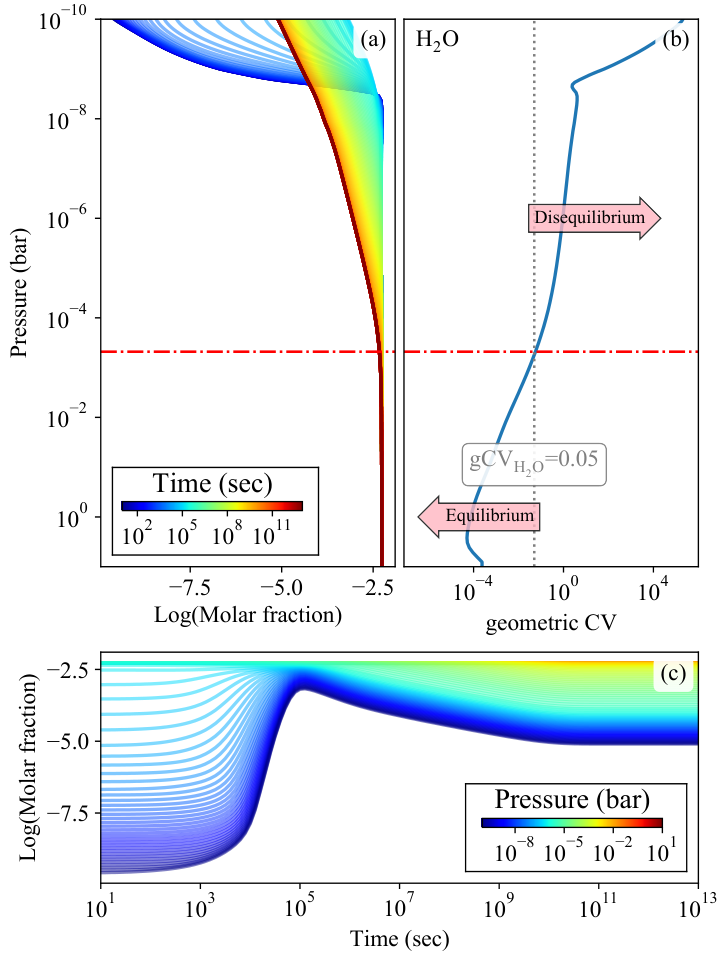
where ${s_{\rm ln}}$ is the sample standard deviation of abundances after a natural log transformation and can be estimated as $s_{\rm ln}=s\ln(10)$ . Stronger variation of abundance at any given altitude results in a higher gCV. We find that gCV ${}_{i}=$ 0.05 represents the onset of disequilibrium chemistry of species $i$ very well, hence gCV ${}_{i}\geq$ 0.05 can be used to mark the regions at which abundances have deviated from their thermochemical equilibrium values significantly. An example is given in Figure 3 based on the results of our diffusion verification model (presented in Figure 15), where water remains in thermochemical equilibrium when gCV_{$\text{H}{\vphantom{\text{X}}}_{\smash[t]{\text{2}}}\text{O}$} $<$ 0.05 (below the red dash-dotted line at $\sim$ 0.5 mbar) and is driven away from it when gCV_{$\text{H}{\vphantom{\text{X}}}_{\smash[t]{\text{2}}}\text{O}$} $\geq$ 0.05 (above $\sim$ 0.5 mbar). The bottom panel in Figure 3 shows the temporal evolution of abundances at different pressures. At the times longer than $t>$ 10¹¹ sec, abundances reach to steady state at all pressures.

We present the results based on the ”quench point from each species”, gCV_i. An alternative method would be to calculate all the timescales relevant for a species at any given pressure. While the alternative method is mathematically correct, our method provides a much simpler picture of the quenching levels based on the actual abundance variation due to the kinetics. Another advantage of our method is that there is no need to trace all the reactions and timescales when calculating the abundances, and the quenching can easily be calculated once the simulations are over. The gCV can be also used in a broader sense to study any abundance deviation from any initial condition as a standard mathematical method for such analysis.

By using this new metric we investigate the quenching levels in our grid of models. Figure 4 (a) shows the density plot of quenching levels of all species in our K_zz=10¹² cm² s^-1 models. In general, P_quench decreases to lower pressures as temperature increases, but its variation at any given temperature is large. For instance, models with T_eff $=$ 2600 K have shown quenching at all pressures ranging from 100 to 10^-8bar in these simulations. But, if we calculate the average P_quench along T_eff (solid black line) the result is similar to the Venot et al. 2018 results of P_quench for K_zz=10¹² cm² s^-1, dashed line in Figure 4 (a).

We find that for a given mixing strength, quenching levels strongly depend on the effective temperature of the planet, but it also depends on the complexity of abundance profiles. For instance, in most cases if a species is the dominant species, then its abundance profile tends to be almost constant. This constant shape of the profiles leads to an underestimation of their P_quench (their abundance does not change very much by mixing since it is constant already, therefore gCV_i remains small at higher pressures and a lower P_quench will be determined). This “constant profiles” region is marked by a dotted line in Figure 4.

The role of T_eff (and K_zz) on the determination of P_quench is rather obvious by following the chemical versus mixing timescale argument; e.g. see Section B.3. However, relating atmospheric parameters to the complexity of abundance profiles is not trivial. Nevertheless, we find that all atmospheric parameters that we have investigated (i.e. T_eff, log(g), [Fe/H], and C/O) affect the complexity of abundance profiles up to some degree. The averaged value of [Fe/H], log(g), and C/O (calculated in each 2D histogram bin represented in the panel (a) of Figure 4) are shown in Figure 4 panels (b), (c), and (d) respectively, to present a graphical demonstration of these dependencies. While Venot et al. 2018 also explored the effect of C/O ratio on the quenching levels, they only found negligible variation. This is mainly due to their narrower parameter-space coverage and their methodology for the determination of the quenching levels as an integrated quantity over the main species.

We will use gCV_i to present an empirical equation for P_quench([Fe/H],log(g),C/O) in a follow-up paper.

III.4 Observability of the disequilibrium chemistry with JWST

One of the key upcoming missions to address the diversity and characterization of exoplanetary atmospheres is JWST. Naturally, the first question would be: “Is there any sweet-spot in the parameter-space to detect the effect of disequilibrium chemistry in the planetary spectra by JWST?”. In order to investigate this, we take a simple approach by subtracting the transmission spectra of each atmospheric model at thermochemical equilibrium and disequilibrium chemistry. The wavelength range spans 0.8 $\mu$ m to 20 $\mu$ m, covering most of the JWST’s wavelength range. The shorter wavelengths, i.e. 0.6 $\mu$ m to 0.8 $\mu$ m, would be likely influenced by the Rayleigh scattering and wavelengths longer than 20 $\mu$ m do not show significant molecular features; hence excluded from this analysis. We then find the maximum spectral deviation for each model due to the disequilibrium.

We should, however, note that using the measured radius at one wavelength is not adequate for a robust detection of disequilibrium fingerprint on the spectra due to the reference pressure degeneracy. Therefore, this analysis should be taken only as a first step toward a spectrum-sensitivity analysis and not a retrieval-degeneracy analysis.

Figure 5 shows an example of the transmission spectra for a Jupiter-sized planet around a G5-type star, with solar metallicity, C/O $\sim$ 0.5, and a surface gravity of 3.5 under two conditions: the thermochemical equilibrium and diffusion equilibrium. The diffusion equilibrium model is shown for K_zz=10¹² cm² s^-1. In this example, the maximum difference between the spectra of the two models, $\Delta$ TD, occurs at the $\text{CH}{\vphantom{\text{X}}}_{\smash[t]{\text{4}}}$ feature at $\sim$ 3.3 $\mu$ m. The difference is about 150 ppm in this model; see the bottom panel of the same figure. While this $\text{CH}{\vphantom{\text{X}}}_{\smash[t]{\text{4}}}$ spectral feature is one of the most prominent features to detect the fingerprints of disequilibrium chemistry, other spectral features from $\text{CH}{\vphantom{\text{X}}}_{\smash[t]{\text{4}}}$ , $\text{H}{\vphantom{\text{X}}}_{\smash[t]{\text{2}}}\text{O}$ , $\text{CO}{\vphantom{\text{X}}}_{\smash[t]{\text{2}}}$ , or CO could be also used as the disequilibrium tracing features. To produce Figure 6, we analyzed where in a spectrum the $\Delta$ TD was maximal for all spectra in the grid and calculated the occurrence at different wavelengths. By finding these occurrence rates we determine which wavelengths are likely to have the highest sensitivity to the vertical mixing. We identify five spectral regions with the highest occurrence rates at $\sim$ 1 $\mu$ m ( $\text{CH}{\vphantom{\text{X}}}_{\smash[t]{\text{4}}}$ , $\text{H}{\vphantom{\text{X}}}_{\smash[t]{\text{2}}}\text{O}$ , or CO), $\sim$ 3.3 $\mu$ m (mostly $\text{CH}{\vphantom{\text{X}}}_{\smash[t]{\text{4}}}$ ), $\sim$ 4.5 $\mu$ m ( $\text{CO}{\vphantom{\text{X}}}_{\smash[t]{\text{2}}}$ or CO), $\sim$ 12 $\mu$ m ( $\text{CH}{\vphantom{\text{X}}}_{\smash[t]{\text{4}}}$ ), and $\sim$ 15 $\mu$ m ( $\text{CH}{\vphantom{\text{X}}}_{\smash[t]{\text{4}}}$ ). Hence, investigation of these wavelengths could provide a higher chance of the detection of disequilibrium spectral signature.

Blumenthal et al. 2018 performed a case study comparing the synthetic emission spectra of HD 189733b, WASP-80b, and GJ 436b. They found that the most significant differences in the emission spectra of these planets within the wavelength rage of 4 to 5 $\mu$ m are due to $\text{CO}{\vphantom{\text{X}}}_{\smash[t]{\text{2}}}$ and CO disequilibrium processes. Although our predictions are based on the synthetic transmission spectra, their results are consistent with our findings for the mentioned wavelength range; see Figure 6.

By averaging the maximum $\Delta$ TD over the free parameters domain, i.e. T_eff, log(g), [Fe/H], C/O ratio, and the spectral type of the star (or alternatively its surface temperature, i.e. T_star), we identify the parameter-space at which the transmission spectra are highly sensitive to the vertical mixing. The results are shown in Figure 7. The T_eff-log(g) panel, at the top-left, suggests a strong dependency of disequilibrium detectability on the surface gravity of the planet. While this is not surprising, this panel shows a higher probability of disequilibrium detection at T_eff between 1000 and 2000 K. This region coincides with the Class-II and Class-III planets, where the evaporation of condensates plays a crucial role in the photospheric chemistry of planets. In fact, all T_eff-dependent results in the left column support this finding. Moreover, the T_eff-C/O panel reveals an interesting trend: as T_eff increases, a higher chance of disequilibrium detectability occurs at higher C/O ratios. More precisely, there is a region around C/O $\sim$ 0.95 with a higher probability of disequilibirum detection. This coincides with the minimum-IR opacity/inversion temperature profiles (Mollière et al. 2015, see e.g.). It appears that such atmospheric condition makes the chemistry to be more easily driven away from its thermochemical equilibrium state. Therefore, this feedback could make the inversion due the minimum-IR opacity, chemically and radiatively unstable. A further self-consistent disequilibirum chemistry calculation must be performed in order to quantitatively assess the significance of this feedback on the inversion.

The T_star-dependent panels, bottom row in Figure 7, illustrate a higher probability of disequilibrium detection when the host stars are colder. This is solely due to the fact that colder stars are associated with smaller radius; hence a larger transit depth for a given planetary radius. The T_star-log(g) panel also suggests that the detection of disequilibrium for a Jupiter-sized planet with high surface gravity maybe only possible for M-dwarfs.

A higher metallicity and C/O ratio results in a higher concentration of carbon-bearing species; in particular $\text{CH}{\vphantom{\text{X}}}_{\smash[t]{\text{4}}}$ , $\text{CO}{\vphantom{\text{X}}}_{\smash[t]{\text{2}}}$ , and CO. Hence, a higher detectability of disequilibrium is expected at these conditions. This is shown in the [Fe/H]-C/O panel, where the region of interest (with dark-blue colors) is associated with super-solar metallicities and super-solar C/O ratios.

In summary, we find that the detectability of disequilibrium could be maximized by focusing on the targets with T_eff between 1000 and 1800 K, orbiting around M-dwarfs, having low surface gravity but high metallicity and a C/O ratio value around unity.

Figure 5: Variation of transmission spectrum due to disequilibrium chemistry for a Jupiter-sized planet orbiting a G5-type star with solar metallicity, C/O

\sim

0.5, and surface gravity of 3.5. Top) Methane abundance decreases as a result of added vertical mixing with K_zz=10¹² cm² s^-1 (blue) with respect to the thermochemical equilibrium state (red). Bottom) The difference between the two spectra indicates that the

\text{CH}{\vphantom{\text{X}}}_{\smash[t]{\text{4}}}

feature at 3.3

\mu

m has the maximum variation within JWST’s wavelength coverage.

Figure 6: Occurrence rate of maximum variation in the transmission spectra, max(

\Delta

TD), within JWST’s wavelength range. Five wavelength regions show the highest occurrences, namely

\sim

\mu

m (

\text{CH}{\vphantom{\text{X}}}_{\smash[t]{\text{4}}}

\text{H}{\vphantom{\text{X}}}_{\smash[t]{\text{2}}}\text{O}

, or CO),

\sim

3.3

\mu

m (mostly

\text{CH}{\vphantom{\text{X}}}_{\smash[t]{\text{4}}}

\sim

4.5

\mu

m (

\text{CO}{\vphantom{\text{X}}}_{\smash[t]{\text{2}}}

or CO),

\sim

\mu

m (

\text{CH}{\vphantom{\text{X}}}_{\smash[t]{\text{4}}}

), and

\sim

\mu

m (

\text{CH}{\vphantom{\text{X}}}_{\smash[t]{\text{4}}}

III.5 Classification and Color-diagram

In the first paper in this series (Molaverdikhani et al. 2019), we proposed a new classification scheme for irradiated gaseous planets based on a grid of cloud-free self-consistent models with four classes. Class-I includes planets colder than 600 $-$ 1100 K. Class-II planets are hotter than Class-I ranging from 600 $-$ 1000 K to about 1650 K. The boundary between Class-I and II changes with log(g), metallicity, and stellar type of the host star. Class-III planets have a temperature between 1650 K and 2200 K, and Class-IV planets are hotter than 2200 K. Here we employ the results of our grid of disequilibrium chemistry models to study the effect of vertical mixing on the atmospheric spectra and hence our proposed classification scheme.

As discussed in the first paper, carbon-to-oxygen ratio affects the composition of hot planetary atmospheres in a way that water is expected to be more prominent at lower C/O ratios and methane, CO, or HCN to be the dominant chemical products at higher C/O ratios. The spectral decomposition technique provides the necessary tool to find the transition C/O ratio, i.e. the C/O ratio at which the atmospheric spectra changes from a water- to methane-dominated spectrum. By employing this technique, we estimate the transition C/O ratios for our grid of disequilibrium chemistry models, see Figure 8, for K_zz=10¹² cm² s^-1 models.

In general, but not always, vertical mixing on Class-II and III planets cause the transition C/O ratios to decrease for atmospheres with high $\beta$ . The $\beta$ factor is a linear combination of surface gravity and metallicity. Higher $\beta$ values represent deeper photospheres, i.e. at higher pressures. See (Molaverdikhani et al. 2019) for a detailed discussion on the $\beta$ factor. This is mostly caused by the higher amount of $\text{CH}{\vphantom{\text{X}}}_{\smash[t]{\text{4}}}$ at the photospheric level, when $\beta$ is higher. Its effect is different for atmospheres with low $\beta$ and vertical mixing increases the transition C/O ratios. These are shown by blue (for low $\beta$ models) and red (for high $\beta$ models) vectors on Figure 8 left panel.

The only difference between Class-II and Class-III planets is that in Class-II the atmosphere still contains some oxygen-bearing condensates, but in Class-III planets all those condensates are evaporated. This causes the transition C/O ratios in Class-III to become independent of atmospheric conditions and remain at a constant value of $\sim$ 0.9. Vertical mixing removes this difference and merges Class-II with III to one extended class; covering the whole range of $\sim$ 900 K to $\sim$ 2000 K in one class.

In Class-I planets, both $\text{H}{\vphantom{\text{X}}}_{\smash[t]{\text{2}}}\text{O}$ and $\text{CH}{\vphantom{\text{X}}}_{\smash[t]{\text{4}}}$ are usually the dominant species and have relatively less vertically variant profiles. Hence, their abundance variation at TOA is less sensitive to the vertical mixing. Class-IV planets with C/O $<$ 1.0 are mostly deficient of $\text{CH}{\vphantom{\text{X}}}_{\smash[t]{\text{4}}}$ due to their hot temperatures. Hence their transition C/O ratio remains higher than unity at all time and are usually insensitive to the vertical mixing. However, some Class-IV planets, T_eff $>$ 2000 K, with very high $\beta$ , $>5$ , show an increase in their transition C/O ratio due to lower $\text{CH}{\vphantom{\text{X}}}_{\smash[t]{\text{4}}}$ abundances at high pressures. Consequently, our proposed four classes of planets based on our grid of cloud-free models can change to a three classification scheme of planets assuming strong vertical mixing in their atmospheres.

Regardless of the naming of these classes, there exists a “Methane Valley” in both thermochemical equilibrium and vertical mixing cases (see Figure 8). The Methane Valley is a region between 800 and 1500 K, where methane is expected to cause the dominant spectral features in the transmission spectra of planets. Hence, a greater chance of $\text{CH}{\vphantom{\text{X}}}_{\smash[t]{\text{4}}}$ detection is expected for the planets within this region. The first robust $\text{CH}{\vphantom{\text{X}}}_{\smash[t]{\text{4}}}$ detection on an irradiated planet was indeed reported for HD 102195b (Guilluy et al. 2019). This is a Class-II planet with T_eq $\sim$ 963 K, within the Methane Valley and consistent with our prediction.

We also calculate the transmission and emission color-maps, using Spitzer IRAC channel 1 and 2, similar to what we presented in the first paper. We note small changes seen in the IRAC emission maps, when going from thermochemical equilibrium to disequilibrium chemistry. Vertical mixing is expected to play a strong role in the atmospheres of cool (T $<$ 1000 K), self-luminous atmospheres with low (planet-like) log(g) (Zahnle & Marley 2014, see, e.g.,). In such atmospheres the abundances of the cooler upper atmospheric layers is overruled by the abundances mixed up from hot layers at higher pressures, which leads to a significant increase in CO abundance, at the expense of $\text{CH}{\vphantom{\text{X}}}_{\smash[t]{\text{4}}}$ . A similar effect appears to occur for a few hundred atmospheres in our grid of $+$ 28,000 models, which start to fill in the region with (F_3.6-F_4.5) $/$ F_4.5 $>$ -0.5. This happens for the models with effective temperatures below $\sim$ 900 K and with very small C/O ratios ( $<$ 0.25) only (blue points in the low C/O regime in Figure 9). Considering what has been predicted for self-luminous atmospheres, this is unexpected. A likely reason for this difference is that the atmospheric temperature profiles of irradiated planets are more isothermal than those of self-luminous ones, such that the deeper (higher pressure) regions from which material is mixed up is cooler, and hence richer in $\text{CH}{\vphantom{\text{X}}}_{\smash[t]{\text{4}}}$ ²² 2 CO to $\text{CH}{\vphantom{\text{X}}}_{\smash[t]{\text{4}}}$ conversion is favored at cool, high pressure conditions; see e.g. Lodders & Fegley 2006; Marley et al. 2002; Hubeny 2017; Noll et al. 2000; Skemer et al. 2012; Saumon et al. 2003..

The color maps do not show any other statistically meaningful differences, see Figure 9, and the two main populations (i.e. $\text{CH}{\vphantom{\text{X}}}_{\smash[t]{\text{4}}}$ -driven and CO/ $\text{CO}{\vphantom{\text{X}}}_{\smash[t]{\text{2}}}$ -driven populations) remain almost invariant. Our results indicate that deviations from the Spitzer equilibrium chemistry color map presented here are most likely due to effects different than the disequilibrium processes studied in our work, with clouds being a strong contender, the effect of which we will study in our upcoming third paper of this series. If disequilibrium should be the culprit for such deviations, it would point to very small C/O ratios ( $<$ 0.25).

IV Conclusion

In this paper, we introduced our newly developed Chemical Kinetic Model (ChemKM). The code includes a variety of atmospheric processes including photolysis, molecular and eddy diffusion, and condensation and rainout. Other processes, such as atmospheric ablation and escape can also be included. It is also possible to include galactic and solar cosmic rays (GCRs) and scattered UV sources by LIPM in the models.

After verification of individual processes in ChemKM, we compared our results to the Venot 2012 model for HD 189733b. The calculated abundances were consistent between the models except at the $\mu$ bar regime, where the molecular diffusion and photochemistry are the dominant processes. As a conclusion, we recommend careful consideration of these processes when abundances at TOA have to be calculated.

We used our grid of disequilibrium chemistry atmospheres with six free parameters, planetary effective temperature (T_eff), surface gravity (log(g)), metallicity ([Fe/H]), carbon-to-oxygen ratio (C/O), spectral type of the host star, and vertical mixing (K_zz=10⁶, 10⁹, and 10¹² cm² s^-1), to determine the quenching levels. We propose a new metric, the geometric Coefficient of variation (gCV) of abundances, for a quantitative measure of quenching. We find P_quench varies significantly under our self-consistent static TP structure setup. We find that all atmospheric parameters ([Fe/H], log(g), and C/O) affect P_quench by changing the atmospheric composition.

To explore the detectability of disequilibrium spectral fingerprints due to the molecular and eddy diffusion by JWST, we recommend focusing on the targets with T_eff between 1000 and 1800 K, orbiting around M-dwarfs, having low surface gravity but high metallicity and high C/O (see Section III.4).

We also find that the “Methane Valley” remains largely unchanged by the inclusion of vertical mixing. This is a region between 800 and 1500 K, where a greater chance of $\text{CH}{\vphantom{\text{X}}}_{\smash[t]{\text{4}}}$ detection is expected. Indeed, the first robust $\text{CH}{\vphantom{\text{X}}}_{\smash[t]{\text{4}}}$ detection on an irradiated planet was within this region (Guilluy et al. 2019); supporting our prediction from Molaverdikhani et al. 2019. We argued in Paper-I that the detection of $\text{CH}{\vphantom{\text{X}}}_{\smash[t]{\text{4}}}$ or the lack of such detection, could hint at the prevalence of cloud formation or disequilibrium chemistry. Here we find that disequilibrium unlikely to change this picture significantly. Thus, characterization of planetary atmospheres within this parameter space is expected to provide a diagnostic tool to identify cloud formation condition.

Our further analysis showed that the two main populations in the Spitzer IRAC’s emission color-maps remain largely unchanged, when including mixing. Although we note some differences between the two maps for the models with effective temperatures below $\sim$ 900 K and with very small C/O ratios ( $<$ 0.25), see Figure 9. Therefore any deviation of observational points from these color-maps is likely to be due to the presence of clouds and not disequilibrium chemistry, but the effect of mixing for cold planets with very low C/O ratios could be significant.

Clouds can potentially change the TP structure, composition, and ultimately the spectra of planetary atmospheres. In the next paper in this series, “From cold to hot irradiated gaseous exoplanets”, we investigate how cloud formation affect the atmospheric spectra and what types of planets are most affected by this process.

V Acknowledgment

The authors would like to thank Dr. Dmitry A. Semenov for constructive feedbacks during the development of ChemKM and would like to thank Dr. Olivia Venot, Dr. Juliane Moses, Dr. Eric Hébrard, and Dr. Shang-Min Tsai for providing their chemical networks. We used the online database KIDA for some kinetic data. This research has made use of the NASA Exoplanet Archive, which is operated by the California Institute of Technology, under contract with the National Aeronautics and Space Administration under the Exoplanet Exploration Program. The authors would like to thank the anonymous reviewer for her/his helpful and constructive comments that greatly contributed to improving the final version of the paper.

VI Softwares

Employed softwares and packages in this work are as follow:

Appendix A Methodology

A.1 Chemical solvers

The challenge of most chemical kinetic models is to find an efficient method to solve the system of ODEs, which are stiff and sparse in nature. Diversity of physical and computational complexities in the simulation of planetary atmospheres results in different degrees of stiffness, and hence complicates the choice of a fast and yet accurate sparse-stiff ODE solver. We have examined two well-established ODE solver packages from the ODEPACK collection, namely DLSODE (Double precision Livermore Solver for Ordinary Differential Equations) and DVODPK (Double precision Variable-coefficient method for Ordinary Differential equations using Preconditioned Krylov method) (Hindmarsh 1983).

The DLSODE solver is based on the older GEAR and GEARB packages, and has the same numerical core. In GEAR, the error is controlled only by one scalar relative error tolerance, called EPS. In DLSODE, on the other hand, the user can set both relative and absolute error tolerances, rtol and atol, which optionally can be scalar or vector. The choice of these error tolerances are usually a compromise between the accuracy and speed of the simulation, i.e. a smaller error tolerance makes the solutions more accurate, but at the same time it increases the computational time, because the solver requires more iterations to achieve the specified tolerance. Our extensive examination of rtol and atol indicates that the computational time scales with rtol exponentially, but the choice of atol has no significant effect on the computational time. Therefore, we choose a very small atol, $10^{-99}$ , as the default atol value for our simulations.

A choice of rtol $=10^{-1}$ , $10^{-2}$ or $10^{-3}$ can be used for a rapid verification of the system’s behavior, but we recommend rtol $=10^{-5}$ to insure numerical stability when the production and loss terms are large, but of the same order, i.e. the system is at or close to $\sim$ steady state, see Figure 10. In this figure we present a worst case scenario where the atmosphere is initialized at its equilibrium state and is forced to remain at that condition by using chemical kinetic calculations. This is not the usual setup and planetary models normally include at least one disequilibrium process such as diffusion. The numerical instability at rtol $=10^{-1}$ and $10^{-3}$ are shown in Figure 10 are for $\text{CH}{\vphantom{\text{X}}}_{\smash[t]{\text{4}}}$ abundance profiles but almost all other species behave similarly. Diffusion usually relaxes the limit on rtol for achieving the numerical stability and introduces a damping effect. In addition, stronger diffusion forces the system to reach the steady state faster; leading to less propagated numerical errors in the steady state solution of the system. Hence, a lower rtol can be selected when stronger diffusion mechanism are in play.

It is also possible to specify the tolerances as vectors; i.e. assigning each species its own relative and absolute tolerances. This treatment could be used, for instance, on a reactant that is completely depleted in at least one vertical layer. In this paper, we use scalar values for rtol and atol with the values of $10^{-5}$ and $10^{-99}$ , respectively.

DVODPK employs iterative methods to solve linear algebraic systems. It is based on orthogonal projection techniques, which approximate a solution of the linear system from a Krylov subspace. This technique is more advanced and more efficient in comparison with DLSODE’s method (Nejad 2005), however, its usage requires decomposition and initialization of the Jacobian matrix. This is not a trivial task and our investigations revealed that this technique requires adaptation of the Jacobian decomposition for every new simulation. Moreover, DVODPK’s performance changes significantly with the physical conditions considered in the model, such as inclusion of condensation, ablation, outgassing, etc.

On top of all is DVODPK’s inefficiency under planetary atmosphere conditions. Figure 11 illustrates the DVODPK’s running time for a suite of 0D simulations over a broad range of densities and temperatures. We found DVODPK is less efficient to solve ODEs at higher density and temperature conditions, and hence is not suitable for the application to planetary atmosphere kinetic simulations. Therefore we use DLSODE from the ODEPACK library as our default solver.

A.2 Chemical networks

Answering the question of which set of reactions, i.e. chemical network, must be used in a chemical kinetic model is arguably the most important question that should be addressed before setting up a model. One could establish a chemical network from the scratch by doing a standard literature search for the thermodynamic polynomial coefficients, reaction rate constants, UV cross sections, and branching ratios, or alternatively employ the commonly used networks in the field. Here we took the latter approach as the establishment of a new network is beyond the scope of this study. Currently, nine chemical networks are available in ChemKM: Moses’s Hot Jupiter network (Moses et al. 2011), Venot’s 2012 network (Venot et al. 2012), Hebrard’s Titan network (Hébrard et al. 2012), Hebrard’s C₃H_p network (Hébrard et al. 2013), Venot’s full network (Venot et al. 2015), Vulcan H-C-O network (Tsai et al. 2017), Moses’s ice-giants network (Moses et al. 2018), Venot’s reduced network (Venot et al. 2019), and Pearce’s HCN network (Pearce et al. 2019), which differ in the complexity, size (number of species and reactions), type of chemistry (reversible/irreversible, H-C-O species, H-C-O-N species, HCN network), and the temperature range over which the chemical schemes are valid, see Table 1.

Chemical Network	Elements	Species	Reactions	Reference
Moses Hot Jupiters	H-C-O-N	90	800	Moses et al. 2011
Venot 2012	H-C-O-N	103	963	Venot et al. 2012
Hébrard 2012	H-C-O-N	135	788	Hébrard et al. 2012
Hébrard 2013	H-C-O-N	90	941	Hébrard et al. 2013
Venot 2015	H-C-O-N	238	2011	Venot et al. 2015
VULCAN H-C-O	H-C-O	29	300	Tsai et al. 2017
Moses Ice-giants	H-C-O	69	385	Moses et al. 2018
Venot reduced	H-C-O-N	29	181	Venot et al. 2019
Pearce HCN	H-C-N	11	42	Pearce et al. 2019

Table 1: General characteristics of chemical networks implemented in ChemKM. He and Ar are excluded from the list of species. The reverse reactions calculated by using the thermodynamic principle of microscopic reversibility are not included.

ChemKM is able to handle a variety of reaction types including KIDA’s standard formulations³³ 3 http://kida.obs.u-bordeaux1.fr (e.g. Modified Arrhenius reactions, third body assisted reactions with Troe (Troe 1983; Gilbert et al. 1983), and SRI (Stewart et al. 1989; Kee et al. 1989) falloff functions) as well as Vuitton (Vuitton et al. 2011) and Jasper (Jasper et al. 2007) formulations. Therefore ChemKM can easily accept new networks as the input of models.

A.3 Condensation and rainout

Observations of planets suggest the presence of clouds nearly in all classes of planets with substantial atmosphere. For instance, Venus is fully covered by a thick cloud layer, containing mostly $\text{H}{\vphantom{\text{X}}}_{\smash[t]{\text{2}}}\text{SO}{\vphantom{\text{X}}}_{\smash[t]{\text{4}}}$ particles (Molaverdikhani et al. 2012, e.g.,). On Earth, water clouds produce a patchy scenery, covering about $70\%$ of the surface with optical depth of larger than 0.1 (Stubenrauch et al. 2013, e.g.,). Despite its tenuous atmosphere, conditions on Mars allow for the formation of what is mostly believed to be high-altitude $\text{CO}{\vphantom{\text{X}}}_{\smash[t]{\text{2}}}$ clouds (Clancy & Sandor 1998, e.g.,).

Outer planets in the solar system have even colder atmospheres, resulting in more efficient cloud-forming environments. Observations and simulations support the formation of $\text{NH}{\vphantom{\text{X}}}_{\smash[t]{\text{3}}}$ , $\text{NH}{\vphantom{\text{X}}}_{\smash[t]{\text{4}}}\text{SH}$ , and $\text{H}{\vphantom{\text{X}}}_{\smash[t]{\text{2}}}\text{O}$ Jovian clouds above 10 bar. Their altitude and thickness, however, could vary both spatially and temporally (Pater et al. 2016). Clouds with similar compositions are expected to form on Saturn; owing to their similarities in temperature structure and bulk composition. However, there are some subtle differences that result in vertically more extended clouds and higher amount of gas above the cloud-bases on Saturn (West et al. 2009; Atreya et al. 1999). Saturn and Neptune observations also show evidence of $\text{CH}{\vphantom{\text{X}}}_{\smash[t]{\text{4}}}$ and $\text{H}{\vphantom{\text{X}}}_{\smash[t]{\text{2}}}\text{S}$ clouds in addition to $\text{NH}{\vphantom{\text{X}}}_{\smash[t]{\text{3}}}$ , $\text{NH}{\vphantom{\text{X}}}_{\smash[t]{\text{4}}}\text{SH}$ , and $\text{H}{\vphantom{\text{X}}}_{\smash[t]{\text{2}}}\text{O}$ clouds, due to their colder environments (Irwin et al. 2018; Irwin et al. 2019).

Although not a planet anymore, Pluto, as seen by the New Horizon spacecraft, is covered by layers of hazes (Gladstone et al. 2016; West 2017), likely due to condensation of hydrocarbons and nitriles such as $\text{C}{\vphantom{\text{X}}}_{\smash[t]{\text{2}}}\text{H}{\vphantom{\text{X}}}_{\smash[t]{\text{2}}}$ , $\text{C}{\vphantom{\text{X}}}_{\smash[t]{\text{2}}}\text{H}{\vphantom{\text{X}}}_{\smash[t]{\text{4}}}$ , $\text{C}{\vphantom{\text{X}}}_{\smash[t]{\text{2}}}\text{H}{\vphantom{\text{X}}}_{\smash[t]{\text{6}}}$ , and HCN (Gao et al. 2017). We also have to mention Titan, since it has a unique and substantial atmosphere, with hydrocarbon and nitrile cloud types. This includes HCN, $\text{HC}{\vphantom{\text{X}}}_{\smash[t]{\text{3}}}\text{N}$ , $\text{CH}{\vphantom{\text{X}}}_{\smash[t]{\text{4}}}$ , $\text{C}{\vphantom{\text{X}}}_{\smash[t]{\text{2}}}\text{H}{\vphantom{\text{X}}}_{\smash[t]{\text{2}}}$ , and $\text{C}{\vphantom{\text{X}}}_{\smash[t]{\text{2}}}\text{H}{\vphantom{\text{X}}}_{\smash[t]{\text{6}}}$ coated particles (Lavvas et al. 2011).

Clouds on gaseous planets beyond the solar system have also been observed. Sing et al. 2016 studied the transmission spectra of 10 Hot Jupiters and concluded that there is very likely a continuum of exoplanetary atmospheres; covered by haze and clouds with a variety of compositions. For instance, a nearly flat transmission spectrum of GJ 1214b (a sub-Neptune planet with an equilibrium temperature of 580 K) is consistent with a planet which is fully covered by clouds; most likely composed of ZnS and KCl (Kreidberg et al. 2014). Hotter Class-II gaseous exoplanets⁴⁴ 4 See the first paper in this series for the classification scheme (Molaverdikhani et al. 2019). with a temperature range of $\sim$ 1000 K to $\sim$ 1650 K could have $\text{Na}{\vphantom{\text{X}}}_{\smash[t]{\text{2}}}\text{S}$ , MnS, Fe, Al $-$ oxides, or silicate clouds such as $\text{Mg}{\vphantom{\text{X}}}_{\smash[t]{\text{2}}}\text{SiO}{\vphantom{\text{X}}}_{\smash[t]{\text{3}}}$ and $\text{Mg}{\vphantom{\text{X}}}_{\smash[t]{\text{2}}}\text{SiO}{\vphantom{\text{X}}}_{\smash[t]{\text{4}}}$ clouds. Even Ultra-Hot Jupiters (T $\gtrsim$ 2500 K) are expected to have cloud formation on their nightside (Helling et al. 2019; Keating & Cowan 2018), which could be dragged toward the dusk terminator of the planet and potentially contribute in the transmission spectra and transit depth of these planets (e.g. Helling in perp.). For a recent review on exoplanet cloud formation see Helling 2019.

All these studies suggest the importance of condensation and particle formation in planetary atmosphere models. However, including even a simplified microphysiscs model, such as atmospheric models by Rossow 1978, in a chemical kinetic model demands high computational resources mostly because of the shorter timescales that condensation and evaporation operate on relative to the vapor transport or gas-phase chemistry timescales (Moses 2014). Hence a simpler approach is usually taken.

Dobrijevic et al. 2010 assumed condensation of species when their abundances reach their saturation level. After hitting this condition, they did not solve the continuity equation of that species at the given altitude; resulting in numerical stability and high computational efficiency of the scheme. A consequence of this approach is that the abundance of the condensed species follows its saturation curve perfectly. But condensation processes could occur at different saturation levels. Capillary condensation is an example, which through this mechanism the vapor condensation occurs below the saturation vapor pressure (Stokes & Evans 1997).

Moses et al. 2000a; Moses et al. 2000b treated the condensed phase of a species as a separate species that is produced by condensation and lost by evaporation through the following reactions:

{}\mathrm{species}\hskip 0.86108pt{}{}\mathrm{(}\mathrm{g}\mathrm{)}{}+{}{}\mathrm{dust}{}\mathrel{\mathop{\makebox[0.0pt]{\rightarrow\displaystyle}}\limits}{}{}\mathrm{species}\hskip 0.86108pt{}{}\mathrm{(}\mathrm{s}\mathrm{)}

(A1)

{}\mathrm{species}\hskip 0.86108pt{}{}\mathrm{(}\mathrm{s}\mathrm{)}{}+{}{}\mathrm{V}{}\mathrel{\mathop{\makebox[0.0pt]{\rightarrow\displaystyle}}\limits}{}{}\mathrm{species}\hskip 0.86108pt{}{}\mathrm{(}\mathrm{g}\mathrm{)}

(A2)

where “dust” represents the condensation nuclei (CN) and must be provided, “V” represents a dummy molecule and its number density assumed to be 1 cm^-3 at all atmospheric levels, and the subscripts (g) and (s) refer to the gas and condensed phases, respectively. This scheme assumes the pre-existence of CN in the atmosphere; allowing the condensation of materials on these sites. They estimated the rate of these reactions by assuming steady-state diffusion-limited condensation and followed Seinfeld 1986 rate estimations.

We follow a similar approach to account for the condensation, but with slightly different rate estimations adapted from Seinfeld & Pandis 2012 as follow:

J_{c}=4\pi R_{p}D_{g}(c_{\infty}-c_{s})

(A3)

where $J_{c}$ is the total flow of the species toward the particle (moles sec^-1), $R_{p}$ is the particle’s radius, $D_{g}$ is the diffusivity of the species in the atmosphere, $c_{\infty}$ is the concentration of the species far from the particle, and $c_{s}$ is its vapor-phase concentration at the particle surface. It is evident that when $c_{\infty}>c_{s}$ then the species flows toward the particle and if $c_{\infty}<c_{s}$ it moves away from it. $c_{s}$ can be estimated from the vapour pressure of species at any given temperature (vapour pressure data of more than 1700 substances are provided in Haynes 2016 and being updated regularly). To consider the condensation in ChemKM, the user is only required to provide a list of desired species to condense. The code then internally handles the addition of “dummy” reactions and condensed phase of species.

Gravitational acceleration leads to the settlement of condensed particles, i.e. rainout, which tends to remove the condensed materials from the atmosphere. Hence, not including the rainout could cause some discrepancies between the observations and models. Two well-known cases are the detection of $\text{H}{\vphantom{\text{X}}}_{\smash[t]{\text{2}}}\text{S}$ gas on Jupiter (Niemann et al. 1998) and the presence of gaseous alkalies in cool brown dwarf and exoplanet atmospheres (Marley et al. 2002; Morley et al. 2012; Line et al. 2017; Zalesky et al. 2019). On Jupiter, Fe could deplete all sulphur content from the upper atmosphere through condensation of FeS; leaving no sulphur to form $\text{H}{\vphantom{\text{X}}}_{\smash[t]{\text{2}}}\text{S}$ . Adding a Fe-rainout mechanism, however, could deplete all Fe from those regions, hence allowing $\text{H}{\vphantom{\text{X}}}_{\smash[t]{\text{2}}}\text{S}$ to form. Similarly, on brown dwarfs and exoplanets, retaining the silicates at high altitudes can eventually lead to the formation of alkali feldspars; resulting in the depletion of alkalies from the upper atmosphere. Including silicate-rainout processes could prevent such an outcome by removing the silicates from those regions (Mollière et al. 2015, e.g.,). As an option in ChemKM, this effect can be included by removing the condensates as soon as they condense. A more sophisticated rainout scheme is under development to take into account a proper estimation of the drag force upon the particles and approximation of the settling velocity.

A.4 Ablation and escape

Ablation of micro-meteoroids during atmospheric entry is thought to be a potential source of volatile gases (such as $\text{H}{\vphantom{\text{X}}}_{\smash[t]{\text{2}}}\text{O}$ , CO, $\text{CO}{\vphantom{\text{X}}}_{\smash[t]{\text{2}}}$ , and $\text{SO}{\vphantom{\text{X}}}_{\smash[t]{\text{2}}}$ ) that cannot be maintained at the upper atmosphere of planets otherwise. These species could change the chemistry and dynamics of the upper layers. For instance, photolysis of the ablated water produces hydroxyl radicals (OH) (Moses & Poppe 2017), which can react with many other species and cause new reaction pathways and products. Although the details of such processes (even on Earth) is not fully understood (Hawkes et al. 2008, e.g.,), usually an ablation rate for each species can be estimated based on the observations of the upper atmosphere of planets through a retrieval procedure (Moses 1992; Hörst et al. 2008; Moses & Poppe 2017).

Atmospheric escape is another process in action at the outermost layers of planetary atmospheres. Several atmospheric escape mechanisms have been identified so far; most of which are non-thermal processes, such as pickup by stellar-wind, bulk escape through magnetic flux ropes, or sputtering (Hunten 1982, e.g.,). While these processes could be the dominant escape mechanisms on colder planets (Brain et al. 2015; Jakosky et al. 2015, e.g.,), hydrodynamic escape (as one of the thermal processes) is believed to be, at least, as important as non-thermal mechanisms for hot exoplanets (Salz et al. 2016, e.g.,). Including all these processes into a chemical kinetic model would be a major task and computationally expensive. Thus, a simplified approach (Moses et al. 2018; Dobrijevic et al. 2014; Hébrard et al. 2013, e.g.,) could be useful. In this approximation, an escape rate is provided for each species at the top of the atmosphere (TOA) and species are removed from the uppermost layer by this rate.

Although gaseous planets have no solid surface, a virtual boundary can be defined as well. For the adequately hot planets, the bottom layer can be selected at a high pressure, where the atmosphere remains at thermochemical equilibirum. However, for cold gaseous planets, their upper troposphere, where a cold-trap is formed, is usually selected to set a boundary layer condition for the chemical models as the bottom layer in the kinetic models is usually not at the thermochemical equilibrium and the local atmosphere is likely prone to the disequilibrium processes. This setting provides more flexibility at the bottom layer of chemical models. For instance, it can be used to estimate the vertical $\text{CH}{\vphantom{\text{X}}}_{\smash[t]{\text{4}}}$ vapor flux that makes it past the tropopause cold trap of Uranus and Neptune (Moses et al. 2018, e.g.,).

These processes can be included by setting the flux rate of species at the top of the atmosphere. Similarly, outgassing and deposition can be included by setting the flux rate of species at the bottom boundary layer in ChemKM.

A.5 Cosmic rays and scattered Ly-alpha by LIPM

Galactic and solar cosmic rays (GCRs) are the main source of ionization at altitudes below 55–60 km on Earth (Velinov 1968; Bazilevskaya 2000); shaping Earth’s stratosphere and thermosphere. GCRs are also the main driving factor of Titan’s photochemistry at pressures between 1 and 50 mbar. Particularly GCR-cascade dissociates $\text{N}{\vphantom{\text{X}}}_{\smash[t]{\text{2}}}$ , a crucial process to synthesis nitrogen organics such as HCN (Capone et al. 1983, e.g.,). GCRs have shown to be important on Neptune’s (Selesnick & Stone 1991; Lellouch et al. 1994; Aplin & Harrison 2016, e.g.,), Titan’s (Molina-Cuberos et al. 1999; Yung et al. 1984, e.g.,), and likely exoplanets’ (Helling et al. 2011; Rimmer & Helling 2013; Scheucher et al. 2018, e.g.,) upper atmospheres, too. A list of GCR reactions along with their rate profiles can be provided to the current version of ChemKM for the inclusion of GCRs. A new GCR module is under development to self-consistently calculate the GCR rates.

Isotropic source of stellar background UV radiation and solar Lyman- $\alpha$ photons that are scattered from atomic hydrogen in the local interplanetary medium (LIPM) are important dissociation/ionization sources at weakly irradiated environments (Strobel et al. 1991; Moses 1991; Bishop et al. 1998, e.g.,), such as polar regions and nightside of closely orbiting planets or the entire atmosphere of planets orbiting at large distances from their host stars. A wavelength dependent flux of these irradiation sources can be provided to ChemKM to be included in the model.

A.6 Initialization

Once all desired physics in the model are set up, one should provide the initial conditions for the temperature-pressure (TP) and abundance profiles. The current version of ChemKM only considers the TP structure statically; i.e. the TP structure does not change as abundances evolve with time. Abundances can be initialized with two options: 1) by providing the elemental abundances or 2) by providing the molar fraction of any desired species at t₀=0.

As a first step, it is possible to calculate the thermochemical equilibrium abundances of species through Gibbs free minimization. We use a slightly modified version of petitCODE’s easy_chem module to perform this (Mollière et al. 2017). Alternatively, the thermochemical equilibrium can be achieved through kinetic calculations. The first approach is usually more suitable, unless the temporal evolution of a system to its thermochemical equilibrium state is as of interest.

Finally, depending on what physical processes are considered in the model, other inputs are also required; for instance the vertical mixing coefficient profile for the eddy diffusion or the influx rates.

Figure 12: Numerical integrator’s performance for a simple case. The results are compared with the analytical solution of the system. They agree within the numerical errors.

Appendix B Model verification

B.1 Numerical integrator

We start the verification of the code by showing how the DLSODE numerical integrator performs. Figure 12 shows the numerical and analytical solutions of the following system of ODEs:

\begin{split}\frac{dy_{1}}{dt}=-y_{2}\\ \frac{dy_{2}}{dt}=y_{1}\end{split}

(B1)

where $y_{i}$ is the abundance of species $i$ at any given time, $t$ . Abundance variation of each species depends on one another, hence the system is coupled. The analytical solution of this simple system is as follow, assuming $y_{1}(0)=y_{2}(0)=1.0$ :

\begin{split}y_{1}=Cos(t)-Sin(t)\\ y_{2}=Cos(t)+Sin(t)\end{split}

(B2)

The results of analytical and numerical solutions are in agreement, hence the numerical performance is assured within the numerical errors.

B.2 Thermochemical equilibrium

Because of the relatively high temperatures at the photosphere of most of known giant exoplanets, simulations of their atmospheric chemistry usually require the consideration of reversible reactions in the model. One issue that have been addressed by previous studies as well (e.g. Moses et al. 2011; Venot et al. 2012; Drummond et al. 2016) is the unavailability of rate coefficients for most reverse reactions. A common workaround is to calculate these rates as the ratio between the forward rate constant and the equilibrium constant. The equilibrium constant, therefore, can be calculated by using NASA thermodynamic polynomial coefficients (McBride et al. 2002). Inclusion or exclusion of reverse reactions in ChemKM is optional, but if it is chosen to be included then it follows the above described method to calculate the reverse rate coefficients.

Taking this approach ensures the consistency of kinetics and thermodynamics steady state solutions. Figure 13 shows this consistency and compares the results of a simple 0D model at T=1560 K and P=10 bar for a kinetic chemical model with reversible reactions (curves) and thermodynamic equilibrium calculations (straight thin dotted lines). The kinetic model reaches the thermodynamic equilibrium after 10⁷ sec with molar fractions practically being identical. Initial atomic abundances (red lines) deplete as molecules (blue lines) are being produced. Obviously, the chemical evolution of reactants depends on the choice of chemical network. For this test, and all other verification tests in this section, we employ the Venot et al. 2012 kinetic network as a verified and benchmarked chemical network.

Figure 14 provides a similar comparison for a 1D model. Neither our 0D nor the 1D model includes mixing or photolyses for these two tests. The temporal evolution of abundances are color-coded by time where green to red shows the progress in time from 10^-10 sec to 1.6 $\times$ 10¹⁸ sec (beyond the age of universe). We show a chemically important atom, N(⁴S), one oxygen $-$ bearing major opacity molecule, $\text{H}{\vphantom{\text{X}}}_{\smash[t]{\text{2}}}\text{O}$ , and one expectedly abundant carbon $-$ bearing molecule at high temperatures, HCN, as examples. It is evident that the abundances at kinetically steady state (dark red) are in agreement with their thermodynamic equilibrium values (gray lines) when the local temperature is adequately high (usually above 1000 K). The N(⁴S) and HCN abundances at pressures between 10^-2 and 10^-8 bar have not fully reached their thermochemical equilibrium and require longer integration times. This shows that the calculation of thermochemical equilibrium is better performed through Gibbs free energy minimization.

As already mentioned, the “kinetically thermochemical equilibrium” mode, i.e. solving the system of ODEs without diffusion or photolyses, can be used as a pre-processing step to initialize the model with thermochemical equilibrium abundances. However, ChemKM has the option to quickly calculate abundances at thermochemical equilibrium by using Gibbs free energy minimization. Figure 10 shows an example of such a setup, where the model is initialized by using Gibbs free energy minimization and all abundances remain the same in the kinetic calculations due to the lack of additional physics such as diffusion or photolyses, hence verifying the validity of our reversible setup to reach or keep the same composition as in thermochemical equilibrium. See Section A.6 for a description of initialization options in ChemKM.

B.3 Molecular and eddy diffusion

Transport-induced quenching is one of the main kinetic-related disequilibrium processes in planetary atmospheres. Both molecular and eddy diffusion could play pivotal roles to drive away the atmospheric composition from their thermochemical equilibrium. If the chemical kinetic timescales are larger than the transport timescales, the mole fraction of a parcel of gas can become quenched in the atmosphere. This usually happens when the temperature and pressure are low enough that the kinetic reactions cannot rapidly occur in both directions; allowing the diffusion processes to drive the system away from its thermochemical equilibrium state.

Figure 15 gives an example for such a system with a 1D atmosphere evolving from its thermochemical equilibrium state. We use the same setup as our 1D example presented in the previous section (Figure 14), but initialize the composition with their thermochemical equilibrium values. We include a vertically constant eddy diffusion (K_zz= $10^{4}$ cm²s^-1) in the model. We choose this relatively low K_zz to demonstrate its significance even in the case of a hot atmosphere (e.g. in this case T_eff=1200 K). No photolyses is included in this setup to only present the effect of diffusion. The abundances reach to a new steady state known as the “diffusion equilibrium” (Lettau 1951, e.g.). A cross-section of Figure 15 at 10^-10 bar is shown in Figure 16 to graphically illustrate the evolution of abundances until they reach the diffusion equilibrium at TOA. Continuing the integration until 10²⁰ sec did not change this new steady state within numerical errors; hence we conclude that this state is a real diffusion equilibrium.

The quenching levels of of O(¹D), N(⁴S),NO, $\text{CH}{\vphantom{\text{X}}}_{\smash[t]{\text{4}}}$ , $\text{CO}{\vphantom{\text{X}}}_{\smash[t]{\text{2}}}$ , CO, see Figure 15, are in agreement with the general estimations of quenching levels in Venot et al. 2018. The quenching level of each constituent, however, depends on its chemical kinetics timescales, ranging from 1 to 10^-3 bar in this example.

A commonly used definition of the “quenching point” (a.k.a. quenching pressure or quenching level) is that the composition of all species remain constant above that level, that is the abundances remain the same as their abundances of their quenching point (Moses 2014, e.g.). This assumption has been also used to mimic a parameterization of disequilibrium processes, usually in the retrieval models as a trade-off to gain more speed (Madhusudhan & Seager 2011, e.g.). However, a constant abundance profile is rarely the case in realistic planetary atmospheres and atmospheric constituent abundances could show significant deviations from their quenched abundances. Prominent processes at mbar level, such as molecular diffusion or photolysis, could drive the abundance profiles away from an idealized constant profile. A non-isothermal TP structure, for example a hot thermosphere with local heating at TOA (as it is the case in the current example, see the TP structure in Figure 14 ), can result in a variation of chemical timescales at different altitudes and might trigger the system to move in and out of thermochemical equilibrium. Including the vertical diffusion causes mixing of these abundances at different pressures; potentially keeping them away from a constant profile. For instance, dissociation of $\text{H}{\vphantom{\text{X}}}_{\smash[t]{\text{2}}}\text{O}$ at TOA due to a hot upper thermosphere depletes its abundances at higher pressures through vertical mixing, see Figure 15 and Figure 3.

In addition, such sharp temperature gradient could also enhance the molecular diffusion (see Equation 2), resulting in more deviation from a constant abundance profile. The left panel of Figure 15 represents such examples, where abundances do not remain constant above their quenching points (black stars) both due to molecular diffusion and thermal $-$ dissociation. More discussion will follow in Section III.3. As a rule of thumb, a constant quenched abundance profile is likely to be valid when the chemical kinetics timescale is much shorter than the timescale of all other processes at all pressures above the quenching point.

B.4 Photochemistry

Photochemistry is another prominent disequilibrium process in planetary atmospheres. We examine the same case as in the previous section, but include photochemistry instead of diffusion. We use an updated version of Hébrard et al. 2012 photolysis reactions (originally adapted from the MPI-Mainz UV/VIS Spectral Atlas Keller-Rudek et al. 2013) and a stellar flux similar to the average solar flux over an entire solar cycle from Thuillier et al. 2004 as the radiation flux at TOA. We initialize abundances with their thermochemical equilibrium values, identical to the previous section initialization.

Figure 17 shows the effect of photolysis on this model. The photochemical timescales are typically shorter than diffusion processes and hence the photolysis should be the dominant mechanism at TOA. Each species responds to the irradiation differently, depending on its shielding and UV cross-section. Some have excess production through photolysis reactions, e.g. N(⁴S) in this model, some face considerable destruction by this process, e.g. $\text{H}{\vphantom{\text{X}}}_{\smash[t]{\text{2}}}\text{O}$ , and some could have a combination of those depending on the altitude, e.g. HCN.

After some time, the system reaches a new steady state, the “photochemical equilibrium”, balancing between reversible reactions and photodissociation. The required integration time to achieve photochemical equilibrium at all vertical levels strongly depends on the atmospheric temperature structure; with hotter atmospheres tending to reach the photochemical equilibrium faster. This is evident in Figure 17, where reaching the photochemical equilibrium at around 10^-3 bar requires integration times larger than the age of the universe.

Absorption cross-sections, the quantum yields, and the actinic flux⁵⁵ 5 “The quantity of light available to molecules at a particular point in the atmosphere and which, on absorption, drives photochemical processes in the atmosphere.” See Calvert 1990 for more details. at a given altitude determine the photodissociation rate of a photo-reactant. Figure 18 shows the irradiation at TOA and the actinic flux at different pressures. The stellar flux quickly vanishes at wavelengths shorter than 220 nm due to strong UV absorption cross-section of photo-reactants at those wavelengths. The rest of the stellar flux is also affected by Rayleigh scattering in this model.

B.5 Condensation

To demonstrate ChemKM’s ability to capture condensation, we model an atmosphere with a temperature structure similar to that of Neptune. This “cold” case creates a suitable environment to examine this process, although ChemKM is capable of including the condensation for hot planets as well. No diffusion or photolysis is included in this model. We also employ the Venot 2012 kinetic network with no reverse reaction. First, we consider a nearly water-saturated atmosphere. This nearly water-saturated atmosphere would allow the condensation to begin at pressures below the intersection of Neptune’s TP structure and $\text{H}{\vphantom{\text{X}}}_{\smash[t]{\text{2}}}\text{O}$ ’s condensation curve. We initialize the model identical to the Moses et al. 2018 Neptune model, except for He and $\text{H}{\vphantom{\text{X}}}_{\smash[t]{\text{2}}}\text{O}$ abundances, and assume an initial atmospheric composition of 80.8 $\%$ $\text{H}{\vphantom{\text{X}}}_{\smash[t]{\text{2}}}\text{O}$ , 19 $\%$ He, $1.2\times 10^{-3}$ $\text{CH}{\vphantom{\text{X}}}_{\smash[t]{\text{4}}}$ and $8\times 10^{-8}$ CO. The particle size is also assumed to be 0.15 $\mu$ m and fixed, following the Moses et al. 2018 assumption. Figure 19 shows the production of $\text{H}{\vphantom{\text{X}}}_{\smash[t]{\text{2}}}\text{O}$ [s] (water ice) under these circumstances, with the expected condensation rates discussed in Section A.3.

In reality, water condensation in the atmosphere of Neptune occurs at higher pressures ( $\approx$ 0.01-1 bar) due to water undersaturation. However, the temperature increases again at the regions deeper than 1 bar, causing the water to remain in the gas phase and making the $\approx$ 0.01-1 bar region a tropopause “cold-trap”. This is shown for water condensation in Figure 20. The initial abundances for this model are 80.8 $\%$ $\text{H}{\vphantom{\text{X}}}_{\smash[t]{\text{2}}}$ , 19 $\%$ He, and the rest is $\text{CH}{\vphantom{\text{X}}}_{\smash[t]{\text{4}}}$ and CO with molar fraction of $1.2\times 10^{-3}$ and $8\times 10^{-8}$ respectively, identical to the initial conditions in Moses et al. 2018. We allow for the condensation of $\text{H}{\vphantom{\text{X}}}_{\smash[t]{\text{2}}}\text{O}$ , NO, $\text{N}{\vphantom{\text{X}}}_{\smash[t]{\text{2}}}$ , $\text{O}{\vphantom{\text{X}}}_{\smash[t]{\text{2}}}$ , C, HCN, $\text{CH}{\vphantom{\text{X}}}_{\smash[t]{\text{4}}}$ , CO, $\text{CO}{\vphantom{\text{X}}}_{\smash[t]{\text{2}}}$ , $\text{C}{\vphantom{\text{X}}}_{\smash[t]{\text{2}}}\text{H}{\vphantom{\text{X}}}_{\smash[t]{\text{2}}}$ , $\text{C}{\vphantom{\text{X}}}_{\smash[t]{\text{2}}}\text{H}{\vphantom{\text{X}}}_{\smash[t]{\text{4}}}$ , and $\text{C}{\vphantom{\text{X}}}_{\smash[t]{\text{2}}}\text{H}{\vphantom{\text{X}}}_{\smash[t]{\text{6}}}$ for demonstration purposes. Condensation of $\text{C}{\vphantom{\text{X}}}_{\smash[t]{\text{2}}}\text{H}{\vphantom{\text{X}}}_{\smash[t]{\text{2}}}$ and C are shown in Figure 20 as examples. In this setup, carbon condenses at all altitudes. However, most Neptune photochemical models do not allow carbon to condensate. This is to maintain a higher production rate of hydrocarbons, such as $\text{C}{\vphantom{\text{X}}}_{\smash[t]{\text{2}}}\text{H}{\vphantom{\text{X}}}_{\smash[t]{\text{2}}}$ and $\text{C}{\vphantom{\text{X}}}_{\smash[t]{\text{2}}}\text{H}{\vphantom{\text{X}}}_{\smash[t]{\text{6}}}$ .

B.6 Influxes and boundary conditions

Ablation, atmospheric escape, and GCR can be included in ChemKM by setting the influx or production rate of reagents. To demonstrate these capabilities, we use the same Neptune model and initialization as the previous section. We include molecular and eddy diffusion as well as photolysis in this case.

First, we only include an influx of $\text{H}{\vphantom{\text{X}}}_{\smash[t]{\text{2}}}\text{O}$ equal to $2\times 10^{5}$ molecules cm^-2s^-1 (Moses et al. 2018, as discussed in the ) to examine how abundances would change. We initialize the atmospheric composition by its ‘‘photo-diffusion equilibrium’’⁶⁶ 6 The steady state after the inclusion of photochemistry and diffusion in the model. We use the same K_zz and irradiation spectrum as in the Moses et al. 2018 Neptune model. Any deviation from this state will be caused by the imposed influx. Figure 21 shows the time evolution of $\text{H}{\vphantom{\text{X}}}_{\smash[t]{\text{2}}}\text{O}$ , CO, O(¹D) and $\text{C}{\vphantom{\text{X}}}_{\smash[t]{\text{2}}}\text{H}{\vphantom{\text{X}}}_{\smash[t]{\text{2}}}$ abundances. As one might expect, $\text{H}{\vphantom{\text{X}}}_{\smash[t]{\text{2}}}\text{O}$ , CO, and O(¹D) abundances increase, but $\text{C}{\vphantom{\text{X}}}_{\smash[t]{\text{2}}}\text{H}{\vphantom{\text{X}}}_{\smash[t]{\text{2}}}$ remains almost the same, due to the lack of free radical carbon. Diffusion plays a pivotal role and transports the deposited material at TOA to the deeper parts of the atmosphere. In this model, the abundance variations caused by $\text{H}{\vphantom{\text{X}}}_{\smash[t]{\text{2}}}\text{O}$ influx at $10^{-11}$ bar typically require $10^{5}$ - $10^{7}$ sec (weeks to months) to reach $10^{-7}$ bar, where the highest altitude measurements of hydrocarbon mixing ratios have taken place (Moses et al. 2018, e.g.). This time scale would be very different if the required oxygen to explain the observations were supplied by a large cometary impact (Lellouch et al. 2005; Luszcz-Cook & de Pater 2013; Moses et al. 2018, e.g.). These possibilities can be addressed by JWST measurements of Neptune’s composition (Roman et al. 2018; Fletcher et al. 2018, e.g.) or a dedicated mission to ice-giants (Hofstdater et al. 2017, e.g.).

Figure 21: Abundance variations due to

2\times 10^{5}

molecules cm^-2s^-1 water influx at TOA. The model has a temperature structure similar to the Neptune model presented in Figure 20, but we initialize the atmospheric composition by its “photo-diffusion equilibrium”; to study the abundance deviations only due to the water-influx.

In the next case study, we run the same model but include an influx of $2\times 10^{8}$ molecules cm^-2s^-1 CO (see Moses et al. 2018, for the motivation) in addition to $\text{H}{\vphantom{\text{X}}}_{\smash[t]{\text{2}}}\text{O}$ . Under these circumstances, excessive production of free carbon radicals and therefore additional carbon-bearing compounds can be expected. However, individual species at different altitudes might respond to these free radicals differently. Photolysis of incoming $\text{H}{\vphantom{\text{X}}}_{\smash[t]{\text{2}}}\text{O}$ and CO results in the production of free radical H, C, and O; hence an increase in the abundance of their elements is expected (e.g. see the variation of O(¹D) abundances in Figure 22), unless there are sink terms with higher loss rates. As expected, the production of CO and $\text{C}{\vphantom{\text{X}}}_{\smash[t]{\text{2}}}\text{H}{\vphantom{\text{X}}}_{\smash[t]{\text{2}}}$ are enhanced early in the simulation, however, at later times (t $\gtrsim 10^{6}$ sec), $\text{C}{\vphantom{\text{X}}}_{\smash[t]{\text{2}}}\text{H}{\vphantom{\text{X}}}_{\smash[t]{\text{2}}}$ abundances seem to be restored to their initial values. This is, of course, not a universal trend and an examination of $\text{C}{\vphantom{\text{X}}}_{\smash[t]{\text{2}}}\text{H}{\vphantom{\text{X}}}_{\smash[t]{\text{2}}}$ abundance reveals its depletion at pressures between 0.1 and $10^{-7}$ bar. Although CO photodissociation enhances $\text{C}{\vphantom{\text{X}}}_{\smash[t]{\text{2}}}\text{H}{\vphantom{\text{X}}}_{\smash[t]{\text{2}}}$ production by offering additional free carbons, it also shields it at longer timescales and returns the $\text{C}{\vphantom{\text{X}}}_{\smash[t]{\text{2}}}\text{H}{\vphantom{\text{X}}}_{\smash[t]{\text{2}}}$ abundances at TOA to their initial values. This extra shielding also causes the depletion of $\text{C}{\vphantom{\text{X}}}_{\smash[t]{\text{2}}}\text{H}{\vphantom{\text{X}}}_{\smash[t]{\text{2}}}$ at mid-pressures and depletion of $\text{H}{\vphantom{\text{X}}}_{\smash[t]{\text{2}}}\text{O}$ and O(¹D) abundances at TOA.

Figure 22: Similar to Figure 21 but additionally

2\times 10^{8}

molecules cm^-2s^-1 CO influx is included.

Similar to these models, boundaries with fixed molar fractions and vertical profile of influxes of reagents (i.e. production rates) can be easily included in ChemKM’s modeling setup. In the case of GCRs, ChemKM includes a separated module to take into account the effect of Galactic/solar cosmic rays. Vertical profiles of production rates of each species with their branching and yields for each GCR reaction can be provided in the current version of the code (similar to the setup of photolysis module).

References

Agúndez et al. (2012) Agúndez, M., Venot, O., Iro, N., et al. 2012, Astronomy & Astrophysics, 548, A73. https://www.aanda.org/articles/aa/abs/2012/12/aa20365-12/aa20365-12.html
Allen et al. (1981) Allen, M., Yung, Y. L., & Waters, J. W. 1981, Journal of Geophysical Research: Space Physics, 86, 3617
Alonso-Floriano et al. (2019) Alonso-Floriano, F. J., Sánchez-López, A., Snellen, I. a. G., et al. 2019, Astronomy & Astrophysics, 621, A74. https:/articles/aa/abs/2019/01/aa34339-18/aa34339-18.html
Aplin & Harrison (2016) Aplin, K. L., & Harrison, R. G. 2016, Nature Communications, 7, 11976. https://www.nature.com/articles/ncomms11976
Atreya et al. (1999) Atreya, S. K., Wong, M. H., Owen, T. C., et al. 1999, Planetary and Space Science, 47, 1243. http://www.sciencedirect.com/science/article/pii/S0032063399000471
Bazilevskaya (2000) Bazilevskaya, G. 2000, Space Science Reviews, 94, 25. https://doi.org/10.1023/A:1026721912992
Bishop et al. (1998) Bishop, J., Romani, P. N., & Atreya, S. K. 1998, Planetary and Space Science, 46, 1. http://www.sciencedirect.com/science/article/pii/S0032063397001268
Blumenthal et al. (2018) Blumenthal, S. D., Mandell, A. M., Hébrard, E., et al. 2018, The Astrophysical Journal, 853, 138. https://doi.org/10.3847%2F1538-4357%2Faa9e51
Brain et al. (2015) Brain, D. A., McFadden, J. P., Halekas, J. S., et al. 2015, Geophysical Research Letters, 9142. https://agupubs.onlinelibrary.wiley.com/doi/abs/10.1002/2015GL065293%4010.1002/%28ISSN%291944-8007.MAVEN1
Brogi et al. (2018) Brogi, M., Giacobbe, P., Guilluy, G., et al. 2018, Astronomy & Astrophysics, 615, A16. https:/articles/aa/abs/2018/07/aa32189-17/aa32189-17.html
Brogi et al. (2016) Brogi, M., Kok, R. J. d., Albrecht, S., et al. 2016, The Astrophysical Journal, 817, 106. https://doi.org/10.3847%2F0004-637x%2F817%2F2%2F106
Burrows & Sharp (1999) Burrows, A., & Sharp, C. M. 1999, The Astrophysical Journal, 512, 843. http://iopscience.iop.org/article/10.1086/306811/meta
Calvert (1990) Calvert, J. G. 1990, Pure and Applied Chemistry, 62, 2167. https://www.degruyter.com/view/j/pac.1990.62.issue-11/pac199062112167/pac199062112167.xml
Capone et al. (1983) Capone, L. A., Dubach, J., Prasad, S. S., & Whitten, R. C. 1983, Icarus, 55, 73. http://www.sciencedirect.com/science/article/pii/0019103583900519
Changeat et al. (2019) Changeat, Q., Edwards, B., Waldmann, I., & Tinetti, G. 2019, arXiv:1903.11180 [astro-ph], arXiv: 1903.11180. http://arxiv.org/abs/1903.11180
Clancy & Sandor (1998) Clancy, R. T., & Sandor, B. J. 1998, Geophysical Research Letters, 25, 489. https://agupubs.onlinelibrary.wiley.com/doi/abs/10.1029/98GL00114
Danielson (1968) Danielson, R. E. S. 1968, APR. 1-2, 1966. https://ntrs.nasa.gov/search.jsp?R=19680063391
Divine (1974) Divine, N. 1974, Titan atmosphere models, 1973. [Saturn satellite], Tech. rep. https://ntrs.nasa.gov/search.jsp?R=19740008423
Divine (1972) Divine, N. P. 1972, SEE N72-31964 22-34, p. p 1. https://ntrs.nasa.gov/search.jsp?R=19720024315
Dobrijevic et al. (2010) Dobrijevic, M., Cavalié, T., Hébrard, E., et al. 2010, Planetary and Space Science, 58, 1555. http://www.sciencedirect.com/science/article/pii/S0032063310002266
Dobrijevic et al. (2014) Dobrijevic, M., Hébrard, E., Loison, J. C., & Hickson, K. M. 2014, Icarus, 228, 324. http://www.sciencedirect.com/science/article/pii/S001910351300434X
Drummond et al. (2016) Drummond, B., Tremblin, P., Baraffe, I., et al. 2016, Astronomy & Astrophysics, 594, A69. https://www.aanda.org/articles/aa/abs/2016/10/aa28799-16/aa28799-16.html
Encrenaz (1974) Encrenaz, T. H. 1974, Observational constraints on model atmospheres for Uranus and Neptune. https://ntrs.nasa.gov/search.jsp?R=19750037243
Fletcher et al. (2018) Fletcher, L., Encrenaz, T., Orton, G., Moses, J., & Rowe-Gurney, N. 2018, in , B5.4–4–18. http://adsabs.harvard.edu/abs/2018cosp...42E1077F
Fortney et al. (2005) Fortney, J. J., Marley, M. S., Lodders, K., Saumon, D., & Freedman, R. 2005, The Astrophysical Journal Letters, 627, L69. http://iopscience.iop.org/article/10.1086/431952/meta
France et al. (2016) France, K., Loyd, R. O. P., Youngblood, A., et al. 2016, The Astrophysical Journal, 820, 89. https://doi.org/10.3847%2F0004-637x%2F820%2F2%2F89
Gao et al. (2017) Gao, P., Fan, S., Wong, M. L., et al. 2017, Icarus, 287, 116. http://www.sciencedirect.com/science/article/pii/S0019103516306170
Gilbert et al. (1983) Gilbert, R. G., Luther, K., & Troe, J. 1983, Berichte der Bunsengesellschaft für physikalische Chemie, 87, 169. https://onlinelibrary.wiley.com/doi/abs/10.1002/bbpc.19830870218
Gladstone et al. (2016) Gladstone, G. R., Stern, S. A., Ennico, K., et al. 2016, Science, 351, aad8866. https://science.sciencemag.org/content/351/6279/aad8866
Greene et al. (2016) Greene, T. P., Line, M. R., Montero, C., et al. 2016, The Astrophysical Journal, 817, 17. https://doi.org/10.3847%2F0004-637x%2F817%2F1%2F17
Guilluy et al. (2019) Guilluy, G., Sozzetti, A., Brogi, M., et al. 2019, arXiv:1904.04170 [astro-ph], arXiv: 1904.04170. http://arxiv.org/abs/1904.04170
Hawkes et al. (2008) Hawkes, R. L., Milley, E. P., Ehrman, J. M., et al. 2008, in Advances in Meteoroid and Meteor Science, ed. J. M. Trigo-Rodríguez, F. J. M. Rietmeijer, J. Llorca, & D. Janches (New York, NY: Springer New York), 331–336. https://doi.org/10.1007/978-0-387-78419-9_47
Haynes (2016) Haynes, W. M. 2016, CRC Handbook of Chemistry and Physics, 97th edn. (CRC Press), google-Books-ID: bNDMBQAAQBAJ
Helling (2019) Helling, C. 2019, Annual Review of Earth and Planetary Sciences, 47, null. https://doi.org/10.1146/annurev-earth-053018-060401
Helling et al. (2019) Helling, C., Gourbin, P., Woitke, P., & Parmentier, V. 2019, arXiv:1901.08640 [astro-ph], arXiv: 1901.08640. http://arxiv.org/abs/1901.08640
Helling et al. (2011) Helling, C., Jardine, M., & Mokler, F. 2011, The Astrophysical Journal, 737, 38. https://doi.org/10.1088%2F0004-637x%2F737%2F1%2F38
Helling & Rimmer (2019) Helling, C., & Rimmer, P. B. 2019, arXiv:1903.04565 [astro-ph, physics:physics], doi:10.1098/rsta.2018.0398, arXiv: 1903.04565. http://arxiv.org/abs/1903.04565
Hindmarsh (1983) Hindmarsh, A. C. 1983, Scientific Computing, 1, 55. https://computation.llnl.gov/casc/nsde/pubs/u88007.pdf
Hofstdater et al. (2017) Hofstdater, m., Simon, A., Reth, K., & Elliot, J. 2017, Ice Giants Mission Planning, NASA Mission Study JPL D-100520, Solar System Exploration Directorate Jet Propulsion Laboratory. https://www.lpi.usra.edu/icegiants/mission_study/
Hu & Seager (2014) Hu, R., & Seager, S. 2014, The Astrophysical Journal, 784, 63. https://doi.org/10.1088%2F0004-637x%2F784%2F1%2F63
Hu et al. (2012) Hu, R., Seager, S., & Bains, W. 2012, The Astrophysical Journal, 761, 166. https://doi.org/10.1088%2F0004-637x%2F761%2F2%2F166
Hu et al. (2013) —. 2013, The Astrophysical Journal, 769, 6. https://doi.org/10.1088%2F0004-637x%2F769%2F1%2F6
Hubeny (2017) Hubeny, I. 2017, Monthly Notices of the Royal Astronomical Society, 469, 841
Hunten (1982) Hunten, D. M. 1982, Planetary and Space Science, 30, 773. http://www.sciencedirect.com/science/article/pii/0032063382901106
Hébrard et al. (2012) Hébrard, E., Dobrijevic, M., Loison, J. C., Bergeat, A., & Hickson, K. M. 2012, Astronomy & Astrophysics, 541, A21. https://www.aanda.org/articles/aa/abs/2012/05/aa18837-12/aa18837-12.html
Hébrard et al. (2013) Hébrard, E., Dobrijevic, M., Loison, J. C., et al. 2013, Astronomy & Astrophysics, 552, A132. https://www.aanda.org/articles/aa/abs/2013/04/aa20686-12/aa20686-12.html
Hörst et al. (2008) Hörst, S. M., Vuitton, V., & Yelle, R. V. 2008, Journal of Geophysical Research: Planets, 113, doi:10.1029/2008JE003135. https://agupubs.onlinelibrary.wiley.com/doi/abs/10.1029/2008JE003135
Irwin et al. (2018) Irwin, P. G. J., Toledo, D., Garland, R., et al. 2018, Nature Astronomy, 2, 420. https://www.nature.com/articles/s41550-018-0432-1
Irwin et al. (2019) —. 2019, Icarus, 321, 550. http://www.sciencedirect.com/science/article/pii/S0019103518306109
Jakosky et al. (2015) Jakosky, B. M., Grebowsky, J. M., Luhmann, J. G., & Brain, D. A. 2015, Geophysical Research Letters, 42, 8791. https://agupubs.onlinelibrary.wiley.com/doi/abs/10.1002/2015GL065271
Jasper et al. (2007) Jasper, A. W., Klippenstein, S. J., Harding, L. B., & Ruscic, B. 2007, The Journal of Physical Chemistry A, 111, 3932. https://doi.org/10.1021/jp067585p
Keating & Cowan (2018) Keating, D., & Cowan, N. B. 2018, arXiv:1809.00002 [astro-ph], arXiv: 1809.00002. http://arxiv.org/abs/1809.00002
Kee et al. (1989) Kee, R. J., Rupley, F., & Miller, M. 1989, Sandia National Laboratories Report. https://ci.nii.ac.jp/naid/10017172558/
Keller-Rudek et al. (2013) Keller-Rudek, H., Moortgat, G. K., Sander, R., & Sörensen, R. 2013, Earth System Science Data, 5, 365. https://www.earth-syst-sci-data.net/5/365/2013/
Kreidberg et al. (2014) Kreidberg, L., Bean, J. L., Désert, J.-M., et al. 2014, Nature, 505, 69. https://www.nature.com/articles/nature12888
Lavvas et al. (2011) Lavvas, P., Griffith, C. A., & Yelle, R. V. 2011, Icarus, 215, 732. http://www.sciencedirect.com/science/article/pii/S0019103511002582
Lellouch et al. (2005) Lellouch, E., Moreno, R., & Paubert, G. 2005, Astronomy & Astrophysics, 430, L37. https://www.aanda.org/articles/aa/abs/2005/05/aagk052/aagk052.html
Lellouch et al. (1994) Lellouch, E., Romani, P. N., & Rosenqvist, J. 1994, Icarus, 108, 112. http://www.sciencedirect.com/science/article/pii/S0019103584710451
Lettau (1951) Lettau, H. 1951, in Compendium of Meteorology: Prepared under the Direction of the Committee on the Compendium of Meteorology, ed. H. R. Byers, H. E. Landsberg, H. Wexler, B. Haurwitz, A. F. Spilhaus, H. C. Willett, H. G. Houghton, & T. F. Malone (Boston, MA: American Meteorological Society), 320–333. https://doi.org/10.1007/978-1-940033-70-9_27
Line et al. (2011) Line, M. R., Vasisht, G., Chen, P., Angerhausen, D., & Yung, Y. L. 2011, The Astrophysical Journal, 738, 32. https://doi.org/10.1088%2F0004-637x%2F738%2F1%2F32
Line et al. (2017) Line, M. R., Marley, M. S., Liu, M. C., et al. 2017, The Astrophysical Journal, 848, 83. http://stacks.iop.org/0004-637X/848/i=2/a=83
Lodders & Fegley (2002) Lodders, K., & Fegley, B. 2002, Icarus, 155, 393. http://www.sciencedirect.com/science/article/pii/S0019103501967405
Lodders & Fegley (2006) —. 2006, in Astrophysics Update 2, ed. J. W. Mason, Springer Praxis Books (Berlin, Heidelberg: Springer Berlin Heidelberg), 1–28. https://doi.org/10.1007/3-540-30313-8_1
Lou (1973) Lou, G. Y. 1973, Models of earth’s atmosphere (90 to 2500 km), Tech. rep. https://ntrs.nasa.gov/search.jsp?R=19730018598
Luszcz-Cook & de Pater (2013) Luszcz-Cook, S. H., & de Pater, I. 2013, Icarus, 222, 379. http://www.sciencedirect.com/science/article/pii/S0019103512004484
Madhusudhan (2012) Madhusudhan, N. 2012, The Astrophysical Journal, 758, 36
Madhusudhan & Seager (2009) Madhusudhan, N., & Seager, S. 2009, The Astrophysical Journal, 707, 24. https://doi.org/10.1088%2F0004-637x%2F707%2F1%2F24
Madhusudhan & Seager (2011) —. 2011, The Astrophysical Journal, 729, 41. http://stacks.iop.org/0004-637X/729/i=1/a=41
Marley et al. (2002) Marley, M. S., Seager, S., Saumon, D., et al. 2002, The Astrophysical Journal, 568, 335. https://doi.org/10.1086%2F338800
Mayor & Queloz (1995) Mayor, M., & Queloz, D. 1995, Nature, 378, 355. https://www.nature.com/articles/378355a0
McBride et al. (2002) McBride, B. J., Zehe, M. J., & Gordon, S. 2002, NASA Glenn Coefficients for Calculating Thermodynamic Properties of Individual Species, Technical Paper E-13336, NASA, National Aeronautics and Space Administration John H. Glenn Research Center at Lewis Field Cleveland, Ohio 44135-3191. https://www.grc.nasa.gov/WWW/CEAWeb/TP-2002-21556.htm
Miguel & Kaltenegger (2014) Miguel, Y., & Kaltenegger, L. 2014, The Astrophysical Journal, 780, 166. http://stacks.iop.org/0004-637X/780/i=2/a=166
Miguel et al. (2014) Miguel, Y., Kaltenegger, L., Linsky, J. L., & Rugheimer, S. 2014, Monthly Notices of the Royal Astronomical Society, 446, 345
Molaverdikhani et al. (2019) Molaverdikhani, K., Henning, T., & Mollière, P. 2019, The Astrophysical Journal, 873, 32. https://doi.org/10.3847%2F1538-4357%2Faafda8
Molaverdikhani et al. (2012) Molaverdikhani, K., McGouldrick, K., & Esposito, L. W. 2012, Icarus, 217, 648
Molina-Cuberos et al. (1999) Molina-Cuberos, G. J., López-Moreno, J. J., Rodrigo, R., Lara, L. M., & O’Brien, K. 1999, Planetary and Space Science, 47, 1347. http://www.sciencedirect.com/science/article/pii/S0032063399000562
Mollière et al. (2017) Mollière, P., Boekel, R. v., Bouwman, J., et al. 2017, Astronomy & Astrophysics, 600, A10. https://www.aanda.org/articles/aa/abs/2017/04/aa29800-16/aa29800-16.html
Mollière et al. (2015) Mollière, P., van Boekel, R., Dullemond, C., Henning, T., & Mordasini, C. 2015, The Astrophysical Journal, 813, 47
Mollière et al. (2019) Mollière, P., Wardenier, J. P., van Boekel, R., et al. 2019, arXiv:1904.11504 [astro-ph], arXiv: 1904.11504. http://arxiv.org/abs/1904.11504
Morley et al. (2012) Morley, C. V., Fortney, J. J., Marley, M. S., et al. 2012, The Astrophysical Journal, 756, 172. https://doi.org/10.1088%2F0004-637x%2F756%2F2%2F172
Moses (1991) Moses, J. I. 1991, phd, California Institute of Technology. http://resolver.caltech.edu/CaltechETD:etd-08012006-093137
Moses (1992) —. 1992, Icarus, 99, 368. http://www.sciencedirect.com/science/article/pii/001910359290153X
Moses (2014) —. 2014, Phil. Trans. R. Soc. A, 372, 20130073. http://rsta.royalsocietypublishing.org/content/372/2014/20130073
Moses et al. (2000a) Moses, J. I., Bézard, B., Lellouch, E., et al. 2000a, Icarus, 143, 244. http://www.sciencedirect.com/science/article/pii/S001910359996270X
Moses et al. (2018) Moses, J. I., Fletcher, L. N., Greathouse, T. K., Orton, G. S., & Hue, V. 2018, Icarus, 307, 124. http://www.sciencedirect.com/science/article/pii/S0019103517307935
Moses et al. (2000b) Moses, J. I., Lellouch, E., Bézard, B., et al. 2000b, Icarus, 145, 166. http://www.sciencedirect.com/science/article/pii/S0019103599963200
Moses & Poppe (2017) Moses, J. I., & Poppe, A. R. 2017, Icarus, 297, 33. http://www.sciencedirect.com/science/article/pii/S001910351730180X
Moses et al. (2011) Moses, J. I., Visscher, C., Fortney, J. J., et al. 2011, The Astrophysical Journal, 737, 15. https://doi.org/10.1088%2F0004-637x%2F737%2F1%2F15
Nejad (2005) Nejad, L. A. M. 2005, Astrophysics and Space Science, 299, 1. https://doi.org/10.1007/s10509-005-2100-z
Niemann et al. (1998) Niemann, H. B., Atreya, S. K., Carignan, G. R., et al. 1998, Journal of Geophysical Research: Planets, 103, 22831. https://agupubs.onlinelibrary.wiley.com/doi/abs/10.1029/98JE01050
Noll et al. (2000) Noll, K. S., Geballe, T. R., Leggett, S. K., & Marley, M. S. 2000, The Astrophysical Journal, 541, L75. https://doi.org/10.1086%2F312906
Noll & McElroy (1972) Noll, R., & McElroy, M. 1972, Models of Venus atmosphere (1972), Tech. rep. https://ntrs.nasa.gov/search.jsp?R=19730008097
Noll & McElroy (1974) —. 1974, Models of Mars’ atmosphere (1974), Tech. rep. https://ntrs.nasa.gov/search.jsp?R=19750011035
Parmentier et al. (2013) Parmentier, V., Showman, A. P., & Lian, Y. 2013, Astronomy & Astrophysics, 558, A91. https://www.aanda.org/articles/aa/abs/2013/10/aa21132-13/aa21132-13.html
Pater et al. (2016) Pater, I. d., Sault, R. J., Butler, B., DeBoer, D., & Wong, M. H. 2016, Science, 352, 1198. https://science.sciencemag.org/content/352/6290/1198
Pearce et al. (2019) Pearce, B. K. D., Ayers, P. W., & Pudritz, R. E. 2019, The Journal of Physical Chemistry A, doi:10.1021/acs.jpca.8b11323. https://doi.org/10.1021/acs.jpca.8b11323
Pino et al. (2018) Pino, L., Ehrenreich, D., Wyttenbach, A., et al. 2018, Astronomy & Astrophysics, 612, A53. https:/articles/aa/abs/2018/04/aa31244-17/aa31244-17.html
Poling et al. (2000) Poling, B., Prausnitz, J., & Connell, J. O. 2000, The Properties of Gases and Liquids (McGraw Hill Professional), google-Books-ID: E920LnqY2woC
Rimmer & Helling (2013) Rimmer, P. B., & Helling, C. 2013, The Astrophysical Journal, 774, 108. https://doi.org/10.1088%2F0004-637x%2F774%2F2%2F108
Roman et al. (2018) Roman, M. T., Fletcher, L. N., Banfield, D. J., & Gierasch, P. J. 2018, AGU Fall Meeting Abstracts, 31. http://adsabs.harvard.edu/abs/2018AGUFM.P31B..05R
Rossow (1978) Rossow, W. B. 1978, Icarus, 36, 1. http://www.sciencedirect.com/science/article/pii/0019103578900726
Salz et al. (2016) Salz, M., Czesla, S., Schneider, P. C., & Schmitt, J. H. M. M. 2016, Astronomy & Astrophysics, 586, A75. https://www.aanda.org/articles/aa/abs/2016/02/aa26109-15/aa26109-15.html
Saumon et al. (2003) Saumon, D., Marley, M. S., Lodders, K., & Freedman, R. S. 2003, Symposium - International Astronomical Union, 211, 345. https://www.cambridge.org/core/journals/symposium-international-astronomical-union/article/nonequilibrium-chemistry-in-the-atmospheres-of-brown-dwarfs/F67F0F6158934EEBC200D46AE2BF8AF8
Scheucher et al. (2018) Scheucher, M., Grenfell, J. L., Wunderlich, F., et al. 2018, The Astrophysical Journal, 863, 6, arXiv: 1808.02347. http://arxiv.org/abs/1808.02347
Schiff et al. (2014) Schiff, M. H., Jaffe, J. S., & Freundlich, B. 2014, Annals of the Rheumatic Diseases, 73, 1549. https://www.ncbi.nlm.nih.gov/pmc/articles/PMC4112421/
Seager et al. (2005) Seager, S., Liang, M.-C., Parkinson, C. D., & Yung, Y. L. 2005, Proceedings of the International Astronomical Union, 1, 491. https://www.cambridge.org/core/journals/proceedings-of-the-international-astronomical-union/article/exoplanet-atmospheres-and-photochemistry/4D397F3F9D7C839FEE02A2F61A39B0CE
Seinfeld (1986) Seinfeld, J. H. 1986, Atmospheric chemistry and physics of air pollution (Wiley), google-Books-ID: NAhSAAAAMAAJ
Seinfeld & Pandis (2012) Seinfeld, J. H., & Pandis, S. N. 2012, Atmospheric Chemistry and Physics: From Air Pollution to Climate Change (John Wiley & Sons), google-Books-ID: YH2K9eWsZOcC
Selesnick & Stone (1991) Selesnick, R. S., & Stone, E. C. 1991, Geophysical Research Letters, 18, 361. https://agupubs.onlinelibrary.wiley.com/doi/abs/10.1029/90GL02582
Sing et al. (2016) Sing, D. K., Fortney, J. J., Nikolov, N., et al. 2016, Nature, 529, 59
Skemer et al. (2012) Skemer, A. J., Hinz, P. M., Esposito, S., et al. 2012, The Astrophysical Journal, 753, 14. https://doi.org/10.1088%2F0004-637x%2F753%2F1%2F14
Stevenson et al. (2010) Stevenson, K. B., Harrington, J., Nymeyer, S., et al. 2010, Nature, 464, 1161. https://www.nature.com/articles/nature09013
Stewart et al. (1989) Stewart, P. H., Larson, C. W., & Golden, D. M. 1989, Combustion and Flame, 75, 25. http://www.sciencedirect.com/science/article/pii/0010218089900849
Stokes & Evans (1997) Stokes, R. J., & Evans, D. F. 1997, Fundamentals of Interfacial Engineering (John Wiley & Sons), google-Books-ID: QuEeGZpjc9kC
Strobel et al. (1991) Strobel, D. F., Meier, R. R., Summers, M. E., & Strickland, D. J. 1991, Geophysical Research Letters, 18, 689. https://agupubs.onlinelibrary.wiley.com/doi/abs/10.1029/91GL00133
Stubenrauch et al. (2013) Stubenrauch, C. J., Rossow, W. B., Kinne, S., et al. 2013, Bulletin of the American Meteorological Society, 94, 1031. https://journals.ametsoc.org/doi/full/10.1175/BAMS-D-12-00117.1
Thuillier et al. (2004) Thuillier, G., Floyd, L., Woods, T. N., et al. 2004, Advances in Space Research, 34, 256. http://www.sciencedirect.com/science/article/pii/S0273117704002388
Troe (1983) Troe, J. 1983, Berichte der Bunsengesellschaft für physikalische Chemie, 87, 161. https://onlinelibrary.wiley.com/doi/abs/10.1002/bbpc.19830870217
Tsai et al. (2017) Tsai, S.-M., Lyons, J. R., Grosheintz, L., et al. 2017, The Astrophysical Journal Supplement Series, 228, 20. https://doi.org/10.3847%2F1538-4365%2F228%2F2%2F20
Velinov (1968) Velinov, P. 1968, Journal of Atmospheric and Terrestrial Physics, 30, 1891. http://www.sciencedirect.com/science/article/pii/0021916968900317
Venot (2012) Venot, O. 2012, thesis, Bordeaux 1. http://www.theses.fr/2012BOR14610
Venot et al. (2019) Venot, O., Bounaceur, R., Dobrijevic, M., et al. 2019, arXiv:1902.04939 [astro-ph], arXiv: 1902.04939. http://arxiv.org/abs/1902.04939
Venot et al. (2018) Venot, O., Drummond, B., Miguel, Y., et al. 2018, Experimental Astronomy, 46, 101. https://doi.org/10.1007/s10686-018-9597-y
Venot et al. (2015) Venot, O., Hébrard, E., Agúndez, M., Decin, L., & Bounaceur, R. 2015, Astronomy & Astrophysics, 577, A33. https://www.aanda.org/articles/aa/abs/2015/05/aa25311-14/aa25311-14.html
Venot et al. (2012) Venot, O., Hébrard, E., Agúndez, M., et al. 2012, Astronomy & Astrophysics, 546, A43. https://www.aanda.org/articles/aa/abs/2012/10/aa19310-12/aa19310-12.html
Vuitton et al. (2011) Vuitton, V., Yelle, R. V., Lavvas, P., & Klippenstein, S. J. 2011, The Astrophysical Journal, 744, 11. https://doi.org/10.1088%2F0004-637x%2F744%2F1%2F11
Wang et al. (2017) Wang, D., Miguel, Y., & Lunine, J. 2017, The Astrophysical Journal, 850, 199. https://doi.org/10.3847%2F1538-4357%2Faa978e
West (2017) West, R. A. 2017, Nature, 551, 302. https://www.nature.com/articles/551302a
West et al. (2009) West, R. A., Baines, K. H., Karkoschka, E., & Sánchez-Lavega, A. 2009, in Saturn from Cassini-Huygens, ed. M. K. Dougherty, L. W. Esposito, & S. M. Krimigis (Dordrecht: Springer Netherlands), 161–179. https://doi.org/10.1007/978-1-4020-9217-6_7
Yung et al. (1984) Yung, Y. L., Allen, M., & Pinto, J. P. 1984, Astrophysical Journal Supplement Series, 55, 465. http://resolver.caltech.edu/CaltechAUTHORS:20140909-090508298
Zahnle & Marley (2014) Zahnle, K. J., & Marley, M. S. 2014, The Astrophysical Journal, 797, 41. http://stacks.iop.org/0004-637X/797/i=1/a=41
Zalesky et al. (2019) Zalesky, J. A., Line, M. R., Schneider, A. C., & Patience, J. 2019, arXiv:1903.11658 [astro-ph], arXiv: 1903.11658. http://arxiv.org/abs/1903.11658
Zhang & Showman (2018) Zhang, X., & Showman, A. P. 2018, arXiv:1808.05365 [astro-ph], arXiv: 1808.05365. http://arxiv.org/abs/1808.05365