跳到论文正文
W Papers独立论文阅读器 arXiv:1908.09831 论文正文 计算阅读时间 · 0%
引用这篇论文根据当前论文元数据生成,正式投稿前建议核对。


License: arXiv.org perpetual non-exclusive license
arXiv:1908.09831v2 [cond-mat.str-el] 13 May 2020

Pairing instability on a Luttinger surface: A non-Fermi liquid to superconductor transition and its Sachdev-Ye-Kitaev dual

Chandan Setty Thanks: email for correspondence: csetty@ufl.edu Affiliation: Department of Physics, University of Florida, Gainesville, Florida, USA
Abstract

Superconductivity results from an instability of the Fermi surface – contour of poles of the single particle propagator – to an infinitesimally small attraction between electrons. Here, we instead discuss the analogous problem on a model Luttinger surface, or contour of zeros of the Green function. At zero temperature (β→∞\beta\rightarrow\infty) and a critical interaction strength (uc​∞u_{c\infty}) characterized by the residue of self-energy pole, we find that the pair susceptibility diverges leading to a superconducting instability. We evaluate the pair fluctuation partition function and find that the spectral density in the normal state has an interaction-driven, power-law 1ω\frac{1}{\sqrt{\omega}} type, van-Hove singularity (vHS) indicating non-Fermi liquid (NFL) physics. Crucially, in the strong coupling limit (β​u≫1\beta u\gg 1), the leading order fluctuation free energy terms in the normal state of this NFL-SC transition resembles the equivalent (O⁡(1))\left(O(1)\right) terms of the Sachdev-Ye-Kitaev (SYK) model. This free energy contribution takes a simple form −β​F=β​uc​∞−γ​ln​(β​uc​∞)-\beta F=\beta u_{c\infty}-\gamma~\text{ln}\left(\beta u_{c\infty}\right) where γ\gamma is a constant equal to 12\frac{1}{2}. Weak impurity scattering (τ≫β−1\tau\gg\beta^{-1}) leaves the low-energy spectral density unaffected, but leads to an interaction-driven enhancement of superconductivity. Our results shed light on the role played by order-parameter fluctuations in providing the key missing link between Mott physics and strongly coupled toy-models exhibiting gravity duals.

I Introduction

A central notion that captures the failure of single-particle physics in quantum matter is the Luttinger surface (LS) – a contour in momentum space where the many-body Green function, G⁡(p,ω)G(\textbf{p},\omega), vanishes Abrikosov et al. 1965. This lies in contrast to the normal Fermi Liquid (FL) where particle excitations are characterized by poles in the single-particle propagator. The LS has been invoked to reconcile several key experimental observations Timusk and Statt 1999; Yoshida et al. 2006; Vishik et al. 2010; He et al. 2011; Yang et al. 2011; Chakravarty 2010 in the Cuprate-Mott insulator under a single unifying paradigm, including the Luttinger sum rule (LSR) Luttinger 1960; Luttinger and Ward 1960; Oshikawa 2000 and its apparent violation  Dzyaloshinskii 1996; Dzyaloshinskii 2003; Essler and Tsvelik 2002; Konik et al. 2006; Yang et al. 2006; Altshuler et al. 1998; Stanescu and Kotliar 2006; Stanescu et al. 2007; Rosch 2007; Dave et al. 2013; Berthod et al. 2006; Sakai et al. 2009, pseudo-gap and Fermi arcs Yang et al. 2006; Stanescu and Kotliar 2006; Phillips 2006; Valenzuela and Bascones 2007; Norman et al. 2007; Vanacore et al. 2018, spectral weight transfer Phillips 2006; Stanescu et al. 2007, as well as features in the self-energy, Σ⁡(p,ω)\Sigma(\textbf{p},\omega) Scheurer et al. 2018.

A salient property of the LS which gives rise to the aforementioned observations is a divergent Σ⁡(p,ω)\Sigma(\textbf{p},\omega) Abrikosov et al. 1965; Essler and Tsvelik 2002; Konik et al. 2006; Yang et al. 2006; Stanescu and Kotliar 2006; Hong and Phillips 2012; Scheurer et al. 2018. The breakdown of the LSR – a rule which relates the density of electrons at fixed chemical potential to the number of excitations in the FL and whose generalizations were shown to hold in broader contexts Blagoev and Bedell 1997; Yamanaka et al. 1997; Oshikawa 2000; Essler and Tsvelik 2002; Dzyaloshinskii 2003; Seki and Yunoki 2017; Heath and Bedell 2019 – serves as an illustrative example to highlight the consequences of a singular self-energy. While the total particle density equals the area enclosed by the surface of propagator-poles when Σ⁡(p,ω)\Sigma(\textbf{p},\omega) is regular, there is an anomalous contribution to the density, proportional to I=∫G​∂Σ∂ωI=\int G\frac{\partial\Sigma}{\partial\omega}, that averages to zero in a FL Luttinger 1960; Luttinger and Ward 1960; Abrikosov et al. 1965. The integral II counts the excess density in addition to the volume contained inside contours where G⁡(p,ω)G(\textbf{p},\omega) changes sign Abrikosov et al. 1965; Dzyaloshinskii 1996; Dzyaloshinskii 2003 and can, however, be non-vanishing when Σ⁡(p,ω)\Sigma(\textbf{p},\omega) diverges Georges et al. 2001; Stanescu and Kotliar 2006; Dave et al. 2013. These many-body properties follow entirely from explicit electron-electron interactions in the problem.

Nevertheless, the normal state of a superconductor can exhibit anomalies that deviate from a FL even in the absence of explicit electron correlations. This class of phenomena originates from Cooper-pair fluctuations Larkin and Varlamov 2005; Varlamov et al. 2018 and lead to precursor effects wherein certain characteristics of the SC are retained for temperatures T>TcT>T_{c}, and in some cases, can even persist for T≫TcT\gg T_{c}. With knowledge of the fluctuation propagator L⁡(q,ω)L(\textbf{q},\omega) – the fundamental object in the theory of pair fluctuations constructed from the ground state of the system for T>TcT>T_{c} – various measurable quantities can be evaluated systematically and compared with experiment Larkin and Varlamov 2005; Varlamov et al. 2018. Several observations such as paraconductivity, rounding of transverse resistance peak, excess tunneling current, pseudo-gap behavior etc (see Refs. Reggiani et al. 1991; Cimberle et al. 1997, Balestrino et al. 1993, Anderson et al. 1972, for example, as well as  Varlamov et al. 2018; Larkin and Varlamov 2005 for a more detailed review) have been successfully understood via fluctuation physics derived from a free electron Green function. More generic models describing the thermodynamics of fluctuations in multi-band systems have also been examined in the context of MgB2 Koshelev et al. 2005.

In this work, we introduce interactions explicitly by analyzing pairing instability and pair fluctuations on a system with a LS formed by a pole in Σ\Sigma. Unlike the problem of pairing on a Fermi surface, we find a quantum phase transition into the superconducting state at a critical interaction strength (uc​∞u_{c\infty}) where the pair susceptibility diverges. By calculating the pair fluctuation propagator L⁡(q,ω)L(\textbf{q},\omega) and partition-function, we determine the spectral density in the normal state. We find an interaction-driven, power-law 1ω\frac{1}{\sqrt{\omega}} type, van-Hove singularity (vHS) at low energies that signals NFL physics. Hence pair fluctuations combined with LS physics describe a NFL-SC transition at T=0T=0. As a key feature we find that, in the strong coupling limit (β​u≫1\beta u\gg 1), the leading order fluctuation free energy terms in the normal state of this NFL-SC transition takes a form similar to the equivalent O⁡(1)O(1) free energy terms of the Sachdev-Ye-Kitaev (SYK) model. This free energy contribution is given by −β​F=β​uc​∞−γ​ln​(β​uc​∞)-\beta F=\beta u_{c\infty}-\gamma~\text{ln}\left(\beta u_{c\infty}\right) where γ=12\gamma=\frac{1}{2}. Here uu is the interaction parameter and is equal to square-root of the residue of the self-energy pole. Moreover, we do not require random couplings for our conclusions to hold. In the presence of weak impurity scattering, the low-energy spectral density is unaffected in the strong coupling limit and gives rise to an interaction-driven enhancement of superconductivity. Our results point toward order-parameter fluctuations acting as conduits between Mott physics and strongly coupled toy-models exhibiting gravity duals Maldacena and Stanford 2016; Cotler et al. 2017.

Refer to caption
Figure 1: Bethe-Salpeter equations for the fluctuation propagator (denoted by zig-zag lines) in the particle-particle channel. The shaded (black solid) disk denotes vertex corrections due to impurities (bare interaction). The dashed (solid) lines denote impurity scatterers (electron Green function).

II Model

LSs have been obtained in numerous models in many-body literature, both at a phenomenological level Yang et al. 2006 as well as microscopic Hubbard-type Essler and Tsvelik 2002; Konik et al. 2006; Stanescu and Kotliar 2006; Rosch 2007; Sakai et al. 2009; Eder et al. 2011; Hong and Phillips 2012; Dave et al. 2013; Scheurer et al. 2018 and holographic Edalati et al. 2011a; Edalati et al. 2011b models. Other models study emergent gauge fields in a FL that nevertheless violate the LSR  Sachdev 2016; Senthil et al. 2003; Mei et al. 2012; Punk and Sachdev 2012. The simplest Green function that vanishes along contours in the Brillouin zone has a simple pole in the self-energy and is given by G​(p,ϵn)−1=i​ϵn−ξ⁡(p)−Σ⁡(p,ϵn)G(\textbf{p},\epsilon_{n})^{-1}=i\epsilon_{n}-\xi(\textbf{p})-\Sigma(\textbf{p},\epsilon_{n}), where ξ⁡(p)=ϵ⁡(p)−μ\xi(\textbf{p})=\epsilon(\textbf{p})-\mu is the bare dispersion with chemical potential μ\mu and ϵn\epsilon_{n} is the fermionic Matsubara frequency. We choose a self-energy ansatz motivated by the well-studied Yang-Rice-Zhang model (YRZ) Yang et al. 2006 with a pole structure given by

Σ⁡(p,i​ϵn)=u2i​ϵn+ξ⁡(p).\displaystyle\Sigma(\textbf{p},i\epsilon_{n})=\frac{u^{2}}{i\epsilon_{n}+\xi(\textbf{p})}. (1)

The constant Hartree-Fock potential is dropped as it results in a trivial renormalization of the bands. As evident from the choice of Σ\Sigma, the LS and the bare electron FS occur for the same momenta set by μ\mu at zero energy. This need not be the case in more generic systems where the self-energy can acquire multiple poles each with distinct residues. The square of the interaction, u2u^{2}, is a quantity determined by microscopic parameters of the Hamiltonian. In the presence of impurities, a finite life-time τ\tau is introduced in the Green function. While the YRZ Green function was motivated by a doped spin-liquid, it is nevertheless a popular example of a minimal (phenomenological) model that has a diverging self-energy; hence it forms a workable model of a Luttinger surface. The Bethe-Salpeter equation appearing in Fig. 1 is an equation for vertex correction and is used to define the bosonic fluctuation propagator in the theory of fluctuation superconductivity Larkin and Varlamov 2005. It assumes a knowledge of the full electronic Green function as an input, either obtained phenomenologically, or from a microscopic Hamiltonian. While in the conventional theory of fluctuations, the pair-bubble is approximated by use of the Green function of non-interacting electrons, we use the aforementioned YRZ proposal as our phenomenological input (see also end of Discussion section and the note added after).

Strong coupling (β​u≫1\beta u\gg 1) in clean limit (τ→∞\tau\rightarrow\infty): The fluctuation propagator can be evaluated from Bethe-Salpeter-type equations in the particle-particle channel (see Fig. 1) for momentum q and frequency Ω\Omega as

L−1​(q,Ω)=−g−1+Π⁡(q,Ω)\displaystyle L^{-1}(\textbf{q},\Omega)=-g^{-1}+\Pi(\textbf{q},\Omega) (2)

where −g-g is a constant bare (attractive) interaction vertex and Π⁡(q,Ω)\Pi(\textbf{q},\Omega) is the pair susceptibility. The latter is defined in dd-dimensions as Π⁡(q,Ωk)=1β​(2​π)d​∑ϵn∫dd​p​G​(p+q,ϵn+k)​G​(−p,−ϵn)\Pi(\textbf{q},\Omega_{k})=\frac{1}{\beta(2\pi)^{d}}\sum_{\epsilon_{n}}\int d^{d}\textbf{p}~G(\textbf{p}+\textbf{q},\epsilon_{n+k})G(-\textbf{p},-\epsilon_{n}), where ϵn≡(2​n+1)​π​T\epsilon_{n}\equiv(2n+1)\pi T and Ωk≡2​k​π​T\Omega_{k}\equiv 2k\pi T are the fermionic and bosonic Matsubara frequencies. Substituting G⁡(p,ϵn)G(\textbf{p},\epsilon_{n}) into Π⁡(q,Ω)\Pi(\textbf{q},\Omega) and taking the limit of |q|≡q≪pf|\textbf{q}|\equiv q\ll p_{f}, the Fermi momentum, we obtain for quadratic bands in d=2d=2 (see Appendix A)

Π⁡(q,Ωk)\displaystyle\Pi(\textbf{q},\Omega_{k}) =\displaystyle= ⟨m2​β∑n[(ϵ1+ϵ1′)​(ϵ1′+ϵ2+i​r​cϕ)ϵ1′​(ϵ12−ϵ22−r2​cϕ2+2​i​cϕ​r​ϵ1′)\displaystyle\Bigg\langle\frac{m}{2\beta}\sum_{n}\Big[\frac{(\epsilon_{1}+\epsilon_{1}^{\prime})(\epsilon_{1}^{\prime}+\epsilon_{2}+irc_{\phi})}{\epsilon_{1}^{\prime}(\epsilon_{1}^{2}-\epsilon_{2}^{2}-r^{2}c_{\phi}^{2}+2ic_{\phi}r\epsilon_{1}^{\prime})} (3)
+c.c(1↔2)]⟩,\displaystyle+\text{c.c}~(1\leftrightarrow 2)\Big]\Bigg\rangle,

where we make the replacements ϵ1≡ϵ1​n→ϵn+k\epsilon_{1}\equiv\epsilon_{1n}\rightarrow\epsilon_{n+k} and ϵ2≡ϵ2​n→−ϵn\epsilon_{2}\equiv\epsilon_{2n}\rightarrow-\epsilon_{n}, and introduce primed notation ϵj​n′≡ϵj​n2+u2\epsilon_{jn}^{\prime}\equiv\sqrt{\epsilon_{jn}^{2}+u^{2}}. The angular brackets ⟨…⟩\langle...\rangle denote angular average, and mm and ϕ\phi are the bare electron mass and azimuthal angle respectively. To recover well-known expressions of the pair-susceptibility for a FL, one only needs to take the limit of u→0u\rightarrow 0 (see Appendix B). We now introduce the ratio r=pf​qm≪u,ϵfr=\frac{p_{f}q}{m}\ll u,\epsilon_{f}, where ϵf\epsilon_{f} is the Fermi energy. Performing an expansion in the parameter r/ur/u (strong interactions) and taking the static limit, the inverse fluctuation propagator is

L−1(q,Ω→0)\displaystyle L^{-1}(\textbf{q},\Omega\rightarrow 0) ≃\displaystyle\simeq −g−1+Π(0)​(0,0)+Π(2)​(q,0),\displaystyle-g^{-1}+\Pi^{(0)}(0,0)+\Pi^{(2)}(\textbf{q},0), (4)

where Π(0)​(0,0)=m4​(2​S1−u2​S3)\Pi^{(0)}(0,0)=\frac{m}{4}\left(2S_{1}-u^{2}S_{3}\right), Π(2)​(q,0)=−m​r232​(2​S3−u2​S5)\Pi^{(2)}(\textbf{q},0)=-\frac{mr^{2}}{32}\left(2S_{3}-u^{2}S_{5}\right) and Sν=1β∑ϵn(ϵn2+u2)−ν/2S_{\nu}=\frac{1}{\beta}\sum_{\epsilon_{n}}(\epsilon_{n}^{2}+u^{2})^{-\nu/2}. These sums can be evaluated exactly for odd ν\nu and we obtain for Λ≫u≫T\Lambda\gg u\gg T (see Appendix C)

Sν={1π​ln⁡Λu−2π​K​(0,κ)for ν=1 e−i​π​ν​Γ​(1−ν2)​sin⁡π⁡(1−ν2)uν−1​2​π3/2​[25−ν2​κν−12​K​(ν−12,κ)−Γ⁡(ν−12)]for ν=3,5,...\displaystyle S_{\nu}=\begin{cases}\text{$\frac{1}{\pi}\ln\frac{\Lambda}{u}-\frac{2}{\pi}K(0,\kappa)$}~~~~~~~~~~~~~~~~~~~~~~~~~~~~~~~~~~~~~~~~~~~~~~~~~~~~~~~\text{for $\nu=1$ }\\ \text{$\frac{e^{-i\pi\nu}\Gamma\left(1-\frac{\nu}{2}\right)\sin\pi\left(1-\frac{\nu}{2}\right)}{u^{\nu-1}2\pi^{3/2}}\left[2^{\frac{5-\nu}{2}}\kappa^{\frac{\nu-1}{2}}K\left(\frac{\nu-1}{2},\kappa\right)-\Gamma\left(\frac{\nu-1}{2}\right)\right]$}~~~~~~\text{for $\nu=3,5,..$.}\end{cases} (5)

Here Λ\Lambda is the ultraviolet cut-off of the divergent Matsubara sum for ν=1\nu=1 (plays the role of the Debye frequency ωD\omega_{D} in the conventional BCS theory), κ≡β​u\kappa\equiv\beta u, Γ⁡(x)\Gamma(x) is the gamma function and K⁡(x,y)K(x,y) is the modified Bessel function of the second kind. Substituting for SνS_{\nu} into Eq. 4 for the inverse fluctuation propagator, and expanding the resulting expression in powers of e−κe^{-\kappa} and its polynomial products, we obtain the final expression for L−1​(q,0)L^{-1}(\textbf{q},0) in the clean limit

L−1(q,Ω→0)\displaystyle L^{-1}(\textbf{q},\Omega\rightarrow 0) ≃\displaystyle\simeq −g−1+N0​[ln⁡Λu+π​κ2​e−κ]\displaystyle-g^{-1}+N_{0}\left[\ln\frac{\Lambda}{u}+\sqrt{\frac{\pi\kappa}{2}}e^{-\kappa}\right] (6)
−N0​r212​u2​[1+π​κ38​e−κ].\displaystyle-\frac{N_{0}r^{2}}{12u^{2}}\left[1+\sqrt{\frac{\pi\kappa^{3}}{8}}e^{-\kappa}\right].

Here N0N_{0} is the density of states at the Fermi level in two dimensions. Note that the above expression cannot be adiabatically connected to the FL result Larkin and Varlamov 2005 any longer as it is valid only in the strong coupling limit. There are several conclusions that can be drawn from the structure of the fluctuation propagator above. First, a divergence of the zero frequency, long-wavelength limit of the propagator signals a superconducting instability. At β=∞\beta=\infty and constant Λ\Lambda, this condition is achieved at the quantum critical point u=uc​∞=Λ​e−1N0​gu=u_{c\infty}=\Lambda~e^{-\frac{1}{N_{0}g}}, a form analogous to the thermal BCS-type transition. Hence, interactions can destroy superconductivity even at zero temperature if u>uc​∞u>u_{c\infty}. This must be contrasted with a recent result Esterlis and Schmalian 2019 where SYK-type random electron-phonon couplings lead to pairing instead of the low temperature quantum critical state. The quantum critical point in the current model can indeed be avoided yielding superconducting pairing provided the surface of zeros is partially or fully destroyed. Second, the conformal structure of the theory is highlighted by setting u=uc​∞u=u_{c\infty} where the static, long-wavelength propagator at low but non-zero temperatures takes a familiar form

L−1(q→0,Ω=0)u=uc​∞=N0π​uc​∞2​Te−uc​∞T\displaystyle L^{-1}(\textbf{q}\rightarrow 0,\Omega=0)_{u=u_{c\infty}}=N_{0}\sqrt{\frac{\pi u_{c\infty}}{2T}}e^{\frac{-u_{c\infty}}{T}} (7)

From this expression, it is illuminating to evaluate the fluctuation contribution to the free energy to zeroth order in q above the critical point. Following the procedures described in Larkin and Varlamov 2005; Koshelev et al. 2005 for the case of a single band model and using Eq. 7, we obtain the leading order pair fluctuation free energy

−β​F=β​uc​∞−γ​ln⁡(β​uc​∞).\displaystyle-\beta F=\beta u_{c\infty}-\gamma~\ln(\beta u_{c\infty}). (8)
Refer to caption
Refer to caption
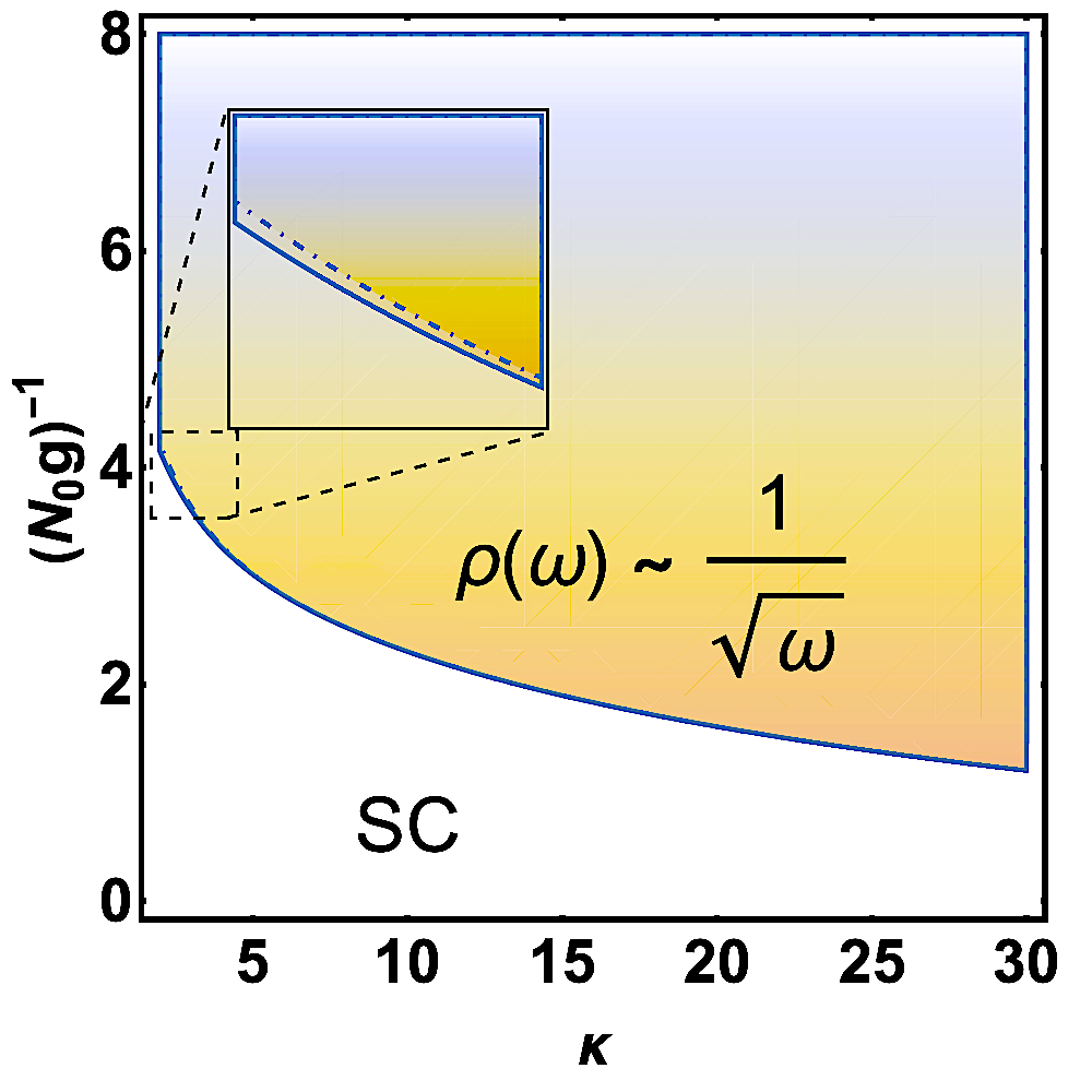
Figure 2: (Left) Schematic plot of the uu-TT phase diagram in the clean limit. The red solid line denotes a Fermi liquid (u=0u=0) while the light (dark) blue contours define the phase boundary in the strong coupling β​u≡κ≫1\beta u\equiv\kappa\gg 1 (weak coupling β​u≪1\beta u\ll 1) limit. The strong coupling normal state is a NFL with a power-law divergence of the spectral density ρ⁡(ω)\rho(\omega). We have defined Tc​0≡Tc​(u=0)T_{c0}\equiv T_{c}(u=0) and uc​∞≡uc​(β→∞)u_{c\infty}\equiv u_{c}(\beta\rightarrow\infty). (Right) Strong coupling, weak impurity scattering (T​τ≡θ≫1T\tau\equiv\theta\gg 1) limit of the κ\kappa-(N0​g)−1(N_{0}g)^{-1} phase diagram. On the solid (dotted-dashed) curve, the pair fluctuations diverge in the absence (presence) of impurity scattering. Inset shows the weak enhancement of SC phase due to impurities.

where γ=12\gamma=\frac{1}{2}. This result must be compared with other quantum critical models having gravity duals such as the Sachdev-Ye-Kitaev (SYK) model and its variants Kitaev 2015; Sachdev and Ye 1993; Sachdev 2010; Maldacena and Stanford 2016; Witten 2016 where the leading order fluctuation contribution to the free energy about the saddle point acquires a form similar to Eq. 8, but with γ=32\gamma=\frac{3}{2} Maldacena and Stanford 2016; Cotler et al. 2017. It is useful to note that the calculated free energy terms should be compared to the O⁡(N0)O(N^{0}) terms in the SYK model (where NN is the number of fermionic flavors) as these are the only contributions that arise from leading order fluctuations about the respective saddle point solutions. Moreover, the fluctuation free energy terms match the SYK results only for the q→0\textbf{q}\rightarrow 0 mode where the spatial dimensionality is smeared out, consistent with an effective zero dimensional model. Hence, and as should be anticipated, it is only in the long-wavelength limit that the proposed mapping of the fluctuation free energy to the O⁡(N0)O(N^{0}) SYK model holds. Finally, one can evaluate the spectral density ρ⁡(ω)\rho(\omega) by taking the inverse Laplace transform of the partition function and the resulting integral can be solved by the saddle point method Maldacena and Stanford 2016. While ρ⁡(ω)\rho(\omega) is a constant independent of ω\omega at low energies in the SYK-type models Maldacena and Stanford 2016, our model yields a vHS ρ⁡(ω)∼1ω\rho(\omega)\sim\frac{1}{\sqrt{\omega}} at low energy leading to NFL transport Davison et al. 2017. This contrast is entirely due to the difference in the coefficient γ\gamma of the log term in Eq. 8. The conclusions drawn above are summarized in Fig. 2. The uu-TT phase diagram in Fig. 2 (left panel) plots the strong coupling phase boundary (solid light blue line) separating the SC and NFL phases for a constant Λ\Lambda. The dashed lines are extrapolations of the phase boundary where approximations made above fail. Fig. 2 (right panel, solid curve) plots the κ\kappa-(N0​g)−1(N_{0}g)^{-1} phase diagram and shows the same phase boundary for close to zero temperatures and constant β​Λ\beta\Lambda. The intensity of fluctuations is indicated by the color scale and is largest in magnitude right above the phase boundary.

Weak coupling (κ=β​u≪1\kappa=\beta u\ll 1) in clean limit (τ→∞\tau\rightarrow\infty): That the T=0T=0 pair instability is only a feature at strong coupling can be confirmed by calculating L−1​(q,0)L^{-1}(\textbf{q},0) in the opposite (weak coupling) limit β​u≪1\beta u\ll 1. We begin with Eq. 4 and expand Π(0)​(0,0)\Pi^{(0)}(0,0) and Π(2)​(q,0)\Pi^{(2)}(\textbf{q},0) to quadratic power in κ=β​u\kappa=\beta u to obtain

Π(0)​(0,0)\displaystyle\Pi^{(0)}(0,0) ≃\displaystyle\simeq m4​β​∑ϵn[2|ϵn|−2​u2|ϵn|3]\displaystyle\frac{m}{4\beta}\sum_{\epsilon_{n}}\left[\frac{2}{|\epsilon_{n}|}-\frac{2u^{2}}{|\epsilon_{n}|^{3}}\right] (9)
Π(2)​(q,0)\displaystyle\Pi^{(2)}(\textbf{q},0) ≃\displaystyle\simeq −m​r232​β​∑ϵn[2|ϵn|3−4​u2|ϵn|5].\displaystyle\frac{-mr^{2}}{32\beta}\sum_{\epsilon_{n}}\left[\frac{2}{|\epsilon_{n}|^{3}}-\frac{4u^{2}}{|\epsilon_{n}|^{5}}\right]. (10)

The sums above can be performed and substituted back into the static limit of the propagator (see Appendix D) and we find,

L−1(q,Ω→0)\displaystyle L^{-1}(\textbf{q},\Omega\rightarrow 0) =\displaystyle= −1g+N0​[ln⁡Λ2​π​T−ψ⁡(12)−u2​C28​π2​T2]\displaystyle-\frac{1}{g}+N_{0}\left[\ln~\frac{\Lambda}{2\pi T}-\psi\left(\frac{1}{2}\right)-\frac{u^{2}C_{2}}{8\pi^{2}T^{2}}\right] (11)
−N0​r2128​π2​T2​[2​C2−u2​C412​π2​T2],\displaystyle-\frac{N_{0}r^{2}}{128\pi^{2}T^{2}}\left[2C_{2}-\frac{u^{2}C_{4}}{12\pi^{2}T^{2}}\right],

where C2=|ψ′′​(12)|C_{2}=|\psi^{\prime\prime}\left(\frac{1}{2}\right)|, C4=|ψ(4)​(12)|C_{4}=|\psi^{(4)}\left(\frac{1}{2}\right)| are numerical constants equal to the second and fourth derivatives of the digamma function ψ⁡(x)\psi(x) respectively. Setting q→0\textbf{q}\rightarrow 0, this form of the fluctuation propagator resembles its thermal BCS counterpart plus the correction term proportional to (β​u)2(\beta u)^{2}. It is hence clear that there is no sensible way to obtain a zero temperature transition into the superconducting state (since β​u≪1\beta u\ll 1). Moreover, as the correction term is negative, its effect on BCS result is to reduce the thermal transition temperature TcT_{c} for a given interaction strength gg and energy cut-off Λ\Lambda. This is shown in Fig. 2 (left panel) where we have defined Tc​0≡Tc​(u=0)T_{c0}\equiv T_{c}(u=0) and the dashed lines are extrapolations of the phase boundary where approximations made above fail.

Strong coupling (β​u≫1\beta u\gg 1) and dilute impurities (θ≡T​τ≫1\theta\equiv T\tau\gg 1): The fluctuation propagator in the presence of impurities is shown in Fig. 1 – the solid lines are now impurity Green functions that acquire zeros and the shaded disk denotes vertex corrections due to impurities. The pair susceptibility bubble then becomes Larkin and Varlamov 2005 (d=2d=2)

Π⁡(q,Ωk)=1β​∑ϵnP⁡(q,ϵ~n+k,−ϵ~n)1−P⁡(q,ϵ~n+k,−ϵ~n)2​π​N0​τ,\displaystyle\Pi(\textbf{q},\Omega_{k})=\frac{1}{\beta}\sum_{\epsilon_{n}}\frac{P(\textbf{q},\tilde{\epsilon}_{n+k},-\tilde{\epsilon}_{n})}{1-\frac{P(\textbf{q},\tilde{\epsilon}_{n+k},-\tilde{\epsilon}_{n})}{2\pi N_{0}\tau}}, (12)

where P⁡(q,ϵ~1,ϵ~2)=1(2​π)2​∫d2​p​G​(p+q,ϵ~1)​G​(−p,ϵ~2)P(\textbf{q},\tilde{\epsilon}_{1},\tilde{\epsilon}_{2})=\frac{1}{(2\pi)^{2}}\int d^{2}\textbf{p}~G(\textbf{p}+\textbf{q},\tilde{\epsilon}_{1})G(-\textbf{p},\tilde{\epsilon}_{2}), ϵ~n=ϵn+sgn​(ϵn)2​τ\tilde{\epsilon}_{n}=\epsilon_{n}+\frac{\text{sgn}(\epsilon_{n})}{2\tau}, and sgn(x)(x) is the sign function. For Ωk=0\Omega_{k}=0, one can perform an expansion in rr similar to the clean case and write

P⁡(q,ϵ~n,−ϵ~n)\displaystyle P(\textbf{q},\tilde{\epsilon}_{n},-\tilde{\epsilon}_{n}) ≃\displaystyle\simeq P(0)​(q=0,ϵ~n,−ϵ~n)+P(2)​(q,ϵ~n,−ϵ~n),\displaystyle P^{(0)}(\textbf{q}=0,\tilde{\epsilon}_{n},-\tilde{\epsilon}_{n})+P^{(2)}(\textbf{q},\tilde{\epsilon}_{n},-\tilde{\epsilon}_{n}),
P(0)​(0,0)\displaystyle P^{(0)}(0,0) =\displaystyle= β​m4​(2​S~1−u2​S~3),\displaystyle\frac{\beta m}{4}\left(2\tilde{S}_{1}-u^{2}\tilde{S}_{3}\right), (13)
P(2)​(q,0)\displaystyle P^{(2)}(\textbf{q},0) =\displaystyle= −β​m​r232​(2​S~3−u2​S~5)\displaystyle-\frac{\beta mr^{2}}{32}\left(2\tilde{S}_{3}-u^{2}\tilde{S}_{5}\right) (14)

and S~ν=1β∑ϵn(ϵ~n2+u2)−ν/2\tilde{S}_{\nu}=\frac{1}{\beta}\sum_{\epsilon_{n}}(\tilde{\epsilon}_{n}^{2}+u^{2})^{-\nu/2}. In the limit β​u≫1\beta u\gg 1 and θ≡T​τ≫1\theta\equiv T\tau\gg 1, the denominator in Eq. 12 can be approximated by unity. This is equivalent to ignoring vertex corrections due to impurity scattering and hence Π⁡(q,Ωk=0)≃1β​∑nP⁡(q,ϵ~n,−ϵ~n)\Pi(\textbf{q},\Omega_{k}=0)\simeq\frac{1}{\beta}\sum_{n}P(\textbf{q},\tilde{\epsilon}_{n},-\tilde{\epsilon}_{n}) (Appendix G gives additional numerical justification for this approximation). The Matsubara sums can be performed exactly for u>τ−1u>\tau^{-1} (Appendix F) and the final expression for the fluctuation propagator is only slightly modified from the clean limit and given by

L−1(q,Ω→0)\displaystyle L^{-1}(\textbf{q},\Omega\rightarrow 0) ≃\displaystyle\simeq −g−1+N0​[ln⁡Λu+π​κ2​e−κ+12​θ]\displaystyle-g^{-1}+N_{0}\left[\ln\frac{\Lambda}{u}+\sqrt{\frac{\pi\kappa}{2}}e^{-\kappa+\frac{1}{2\theta}}\right] (15)
−N0​r212​u2​[1+π​κ38​e−κ+12​θ].\displaystyle-\frac{N_{0}r^{2}}{12u^{2}}\left[1+\sqrt{\frac{\pi\kappa^{3}}{8}}e^{-\kappa+\frac{1}{2\theta}}\right].

Hence its conformal structure at the quantum critical point, L−1(q→0,Ω=0)u=uc​∞=N0π​uc​∞2​Te−uc​∞T+12​θL^{-1}(\textbf{q}\rightarrow 0,\Omega=0)_{u=u_{c\infty}}=N_{0}\sqrt{\frac{\pi u_{c\infty}}{2T}}e^{\frac{-u_{c\infty}}{T}+\frac{1}{2\theta}}, as well as the free energy contribution and vHS in ρ⁡(ω)\rho(\omega) are left essentially unchanged. On the other hand, as shown in Fig. 2 (right panel), there is a weak enhancement of the superconducting phase in the strong coupling phase diagram.

Weak coupling (β​u≪1\beta u\ll 1) and dilute impurities (T​τ≫1T\tau\gg 1): The final case we consider is the weak coupling limit in the presence of dilute impurities. In this limit, vertex corrections become more important than in the strong coupling case (Appendix G) and the static long-wavelength limit of the pair susceptibility is

Π(q→0,Ω=0)\displaystyle\Pi(\textbf{q}\rightarrow 0,\Omega=0) =\displaystyle= 1β​∑n2​π​N0​τ​A~​(ϵ~n,u)2​π​N0​τ−A~​(ϵ~n,u)\displaystyle\frac{1}{\beta}\sum_{n}\frac{2\pi N_{0}\tau\tilde{A}(\tilde{\epsilon}_{n},u)}{2\pi N_{0}\tau-\tilde{A}(\tilde{\epsilon}_{n},u)} (16)
A~​(ϵ~n,u)\displaystyle\tilde{A}(\tilde{\epsilon}_{n},u) =\displaystyle= 2​π​N04​[2ϵ~n′−u2ϵ~n′3].\displaystyle\frac{2\pi N_{0}}{4}\left[\frac{2}{\tilde{\epsilon}_{n}^{\prime}}-\frac{u^{2}}{\tilde{\epsilon}_{n}^{\prime 3}}\right]. (17)

Like in the case of the clean limit, we can perform an expansion in β​u\beta u and the Matsubara summations have been performed in Appendix E. The final result for the fluctuation propagator in this limit takes the form

L−1(q→0,Ω=0)=−g−1+N0[ln(Λ4​π​T)−ψ(12)+4u2τ2[ψ(12+14​π​θ)−14​π​θψ′(12)−ψ(12)]].\displaystyle L^{-1}(\textbf{q}\rightarrow 0,\Omega=0)=-g^{-1}+N_{0}\left[\ln~\left(\frac{\Lambda}{4\pi T}\right)-\psi\left(\frac{1}{2}\right)+4u^{2}\tau^{2}\left[\psi\left(\frac{1}{2}+\frac{1}{4\pi\theta}\right)-\frac{1}{4\pi\theta}\psi^{\prime}(\frac{1}{2})-\psi\left(\frac{1}{2}\right)\right]\right]. (18)

This expression for the propagator looks similar to that obtained in the limit of low q and τ<∞\tau<\infty, but with u2u^{2} replacing the energy scale arising from the squared momentum factor Larkin and Varlamov 2005. In this limit, as anticipated from the clean case, the conformal structure of the propagator is lost and there is only a thermal transition into the superconducting state.

III Discussion

As alluded to in the main text, the near-conformal structure of the fluctuation propagator and the associated free energy (Eqs. 7 and 8) obtained from the YRZ Green function is reminiscent of the SYK model discussed in Ref. Maldacena and Stanford 2016. The difference in the coefficient γ\gamma of the logarithmic term results in a power-law divergence of the spectral density as opposed to a constant as in the SYK model. Moreover, the physics in both cases is controlled by a single parameter in the strong coupling-low temperature limit. In the SYK case, it is the parameter β​J→∞\beta J\rightarrow\infty whereas in the YRZ case its is β​u→∞\beta u\rightarrow\infty. In both scenarios, the respective dualities – SYK to 2-dimensional gravity and YRZ fluctuations to SYK (to leading order in fluctuations)– occur only in the strong coupling limit. Furthermore, although the SYK Green function is local, given by G⁡(i​ωn)=−i​ωn−Σ⁡(i​ωn)G(i\omega_{n})=-i\omega_{n}-\Sigma(i\omega_{n}), as opposed to the momentum dependent YRZ case, the respective free energy terms coincide only for the q→0\textbf{q}\rightarrow 0 YRZ mode where the spatial dimensionality is smeared out, reducing the model to an effectively zero dimensional system like the SYK. The key difference, however, is the absence of any disorder (a result consistent with the conclusion of Ref. Witten 2016) needed in our calculations; instead, we require a momentum-dependent (non-local) self-energy to obtain the same physical content. In addition, a large-NN parameter, typically used in SYK-type models, is absent. We also emphasize that the equivalence between Eqs. 7, 8 and the corresponding quantities in gravity-type models holds without additional vertex corrections from Coulomb interactions. Therefore, these terms are expected to be unimportant for establishing this equivalence (see also note added at the end). Furthermore, the weak enhancement of the superconducting phase induced by the interplay of electron correlations and dilute impurities is also consistent with previous studies Seki 1995; Galitski and Larkin 2002; Setty 2019. Looking ahead, it would be of considerable interest to examine the consequences of fluctuation-driven vHS on properties such as the entanglement entropy and energy-level spacing near the quantum critical point for a model with a LS. Additionally, the difference in the factor γ\gamma in the fluctuation free energy appearing in Eq. 8 suggests a generalization of the Schwarzian action describing in the AdS2×{}_{2}\timesS2 geometry Maldacena and Stanford 2016. This could provide crucial insight into this distinction between fluctuations on a LS and SYK. Finally, while no explicit reference to a microscopic model has been made in this work, the conclusions in this paper are applicable to exactly solvable Hamiltonians hosting LSs such as those in Ref. Hatsugai and Kohmoto 1992. This is the subject of ongoing and future work.

Note Added: After the completion of this work, a follow-up preprint by Phillips and coworkers Phillips et al. 2019 pointed out that an LS of the form similar to the one obtained through the YRZ Green function could also be realized via an exactly solvable microscopic model with long-range interactions by Hatsugai and Kohmoto Hatsugai and Kohmoto 1992. The results appearing in the current paper are applicable to this model in the presence of an additional superconducting interaction term Phillips et al. 2019 and will be addressed in a forthcoming manuscript.

Acknowledgements: We thank P. W. Phillips and G. La Nave for illuminating discussions and B. Padhi for a critical reading of the manuscript. This work is supported by the DOE grant number DE-FG02-05ER46236.

References

  • Abrikosov et al. (1965) A. A. Abrikosov, L. P. Gorkov, and I. E. Dzyaloshinskii, Quantum field theoretical methods in statistical physics, Vol. 4 (Pergamon, 1965).
  • Timusk and Statt (1999) T. Timusk and B. Statt, Reports on Progress in Physics 62, 61 (1999).
  • Yoshida et al. (2006) T. Yoshida, X. Zhou, K. Tanaka, W. Yang, Z. Hussain, Z.-X. Shen, A. Fujimori, S. Sahrakorpi, M. Lindroos, R. Markiewicz, et al., Physical Review B 74, 224510 (2006).
  • Vishik et al. (2010) I. Vishik, W. Lee, R. He, M. Hashimoto, Z. Hussain, T. Devereaux, and Z. Shen, New Journal of Physics 12, 105008 (2010).
  • He et al. (2011) R.-H. He, X. Zhou, M. Hashimoto, T. Yoshida, K. Tanaka, S. Mo, T. Sasagawa, N. Mannella, W. Meevasana, H. Yao, et al., New Journal of Physics 13, 013031 (2011).
  • Yang et al. (2011) H.-B. Yang, J. D. Rameau, Z.-H. Pan, G. D. Gu, P. D. Johnson, H. Claus, D. G. Hinks, and T. E. Kidd, Phys. Rev. Lett. 107, 047003 (2011).
  • Chakravarty (2010) S. Chakravarty, arXiv preprint arXiv:1006.4180 (2010).
  • Luttinger (1960) J. M. Luttinger, Phys. Rev. 119, 1153 (1960).
  • Luttinger and Ward (1960) J. M. Luttinger and J. C. Ward, Physical Review 118, 1417 (1960).
  • Oshikawa (2000) M. Oshikawa, Physical Review Letters 84, 3370 (2000).
  • Dzyaloshinskii (1996) I. Dzyaloshinskii, Journal de Physique I 6, 119 (1996).
  • Dzyaloshinskii (2003) I. Dzyaloshinskii, Physical Review B 68, 085113 (2003).
  • Essler and Tsvelik (2002) F. H. Essler and A. M. Tsvelik, Physical Review B 65, 115117 (2002).
  • Konik et al. (2006) R. Konik, T. Rice, and A. Tsvelik, Physical review letters 96, 086407 (2006).
  • Yang et al. (2006) K.-Y. Yang, T. Rice, and F.-C. Zhang, Physical Review B 73, 174501 (2006).
  • Altshuler et al. (1998) B. Altshuler, A. Chubukov, A. Dashevskii, A. Finkel’stein, and D. Morr, EPL (Europhysics Letters) 41, 401 (1998).
  • Stanescu and Kotliar (2006) T. D. Stanescu and G. Kotliar, Physical Review B 74, 125110 (2006).
  • Stanescu et al. (2007) T. D. Stanescu, P. Phillips, and T.-P. Choy, Physical Review B 75, 104503 (2007).
  • Rosch (2007) A. Rosch, The European Physical Journal B 59, 495 (2007).
  • Dave et al. (2013) K. B. Dave, P. W. Phillips, and C. L. Kane, Physical review letters 110, 090403 (2013).
  • Berthod et al. (2006) C. Berthod, T. Giamarchi, S. Biermann, and A. Georges, Physical review letters 97, 136401 (2006).
  • Sakai et al. (2009) S. Sakai, Y. Motome, and M. Imada, Physical review letters 102, 056404 (2009).
  • Phillips (2006) P. Phillips, Annals of Physics 321, 1634 (2006).
  • Valenzuela and Bascones (2007) B. Valenzuela and E. Bascones, Physical review letters 98, 227002 (2007).
  • Norman et al. (2007) M. Norman, A. Kanigel, M. Randeria, U. Chatterjee, and J. Campuzano, Physical Review B 76, 174501 (2007).
  • Vanacore et al. (2018) G. Vanacore, S. T. Ramamurthy, and P. W. Phillips, Journal of High Energy Physics 2018, 9 (2018).
  • Scheurer et al. (2018) M. S. Scheurer, S. Chatterjee, W. Wu, M. Ferrero, A. Georges, and S. Sachdev, Proceedings of the National Academy of Sciences 115, E3665 (2018).
  • Hong and Phillips (2012) S. Hong and P. Phillips, Physical Review B 86, 115118 (2012).
  • Blagoev and Bedell (1997) K. B. Blagoev and K. S. Bedell, Phys. Rev. Lett. 79, 1106 (1997).
  • Yamanaka et al. (1997) M. Yamanaka, M. Oshikawa, and I. Affleck, Phys. Rev. Lett. 79, 1110 (1997).
  • Seki and Yunoki (2017) K. Seki and S. Yunoki, Phys. Rev. B 96, 085124 (2017).
  • Heath and Bedell (2019) J. T. Heath and K. S. Bedell, arXiv preprint arXiv:1906.00929 (2019).
  • Georges et al. (2001) A. Georges, O. Parcollet, and S. Sachdev, Physical Review B 63, 134406 (2001).
  • Larkin and Varlamov (2005) A. Larkin and A. Varlamov, Theory of fluctuations in superconductors (Clarendon Press, 2005).
  • Varlamov et al. (2018) A. Varlamov, A. Galda, and A. Glatz, Reviews of Modern Physics 90, 015009 (2018).
  • Reggiani et al. (1991) L. Reggiani, R. Vaglio, and A. Varlamov, Physical Review B 44, 9541 (1991).
  • Cimberle et al. (1997) M. Cimberle, C. Ferdeghini, E. Giannini, D. Marre, M. Putti, A. Siri, F. Federici, and A. Varlamov, Physical Review B 55, R14745 (1997).
  • Balestrino et al. (1993) G. Balestrino, E. Milani, and A. Varlamov, Physica C: Superconductivity 210, 386 (1993).
  • Anderson et al. (1972) J. Anderson, R. Carlson, and A. M. Goldman, Journal of Low Temperature Physics 8, 29 (1972).
  • Koshelev et al. (2005) A. Koshelev, A. Varlamov, and V. Vinokur, Physical Review B 72, 064523 (2005).
  • Maldacena and Stanford (2016) J. Maldacena and D. Stanford, Phys. Rev. D 94, 106002 (2016).
  • Cotler et al. (2017) J. S. Cotler, G. Gur-Ari, M. Hanada, J. Polchinski, P. Saad, S. H. Shenker, D. Stanford, A. Streicher, and M. Tezuka, Journal of High Energy Physics 2017, 118 (2017).
  • Eder et al. (2011) R. Eder, K. Seki, and Y. Ohta, Physical Review B 83, 205137 (2011).
  • Edalati et al. (2011a) M. Edalati, R. G. Leigh, and P. W. Phillips, Physical review letters 106, 091602 (2011a).
  • Edalati et al. (2011b) M. Edalati, R. G. Leigh, K. W. Lo, and P. W. Phillips, Physical Review D 83, 046012 (2011b).
  • Sachdev (2016) S. Sachdev, Philosophical Transactions of the Royal Society A: Mathematical, Physical and Engineering Sciences 374, 20150248 (2016).
  • Senthil et al. (2003) T. Senthil, S. Sachdev, and M. Vojta, Physical review letters 90, 216403 (2003).
  • Mei et al. (2012) J.-W. Mei, S. Kawasaki, G.-Q. Zheng, Z.-Y. Weng, and X.-G. Wen, Physical Review B 85, 134519 (2012).
  • Punk and Sachdev (2012) M. Punk and S. Sachdev, Physical Review B 85, 195123 (2012).
  • Esterlis and Schmalian (2019) I. Esterlis and J. Schmalian, Phys. Rev. B 100, 115132 (2019).
  • Kitaev (2015) A. Kitaev, http://online.kitp.ucsb.edu/online/entangled15/kitaev/ (2015).
  • Sachdev and Ye (1993) S. Sachdev and J. Ye, Physical review letters 70, 3339 (1993).
  • Sachdev (2010) S. Sachdev, Physical review letters 105, 151602 (2010).
  • Witten (2016) E. Witten, arXiv preprint arXiv:1610.09758 (2016).
  • Davison et al. (2017) R. A. Davison, W. Fu, A. Georges, Y. Gu, K. Jensen, and S. Sachdev, Physical Review B 95, 155131 (2017).
  • Seki (1995) S. Seki, Progress of Theoretical Physics 94, 181 (1995).
  • Galitski and Larkin (2002) V. Galitski and A. Larkin, Physical Review B 66, 064526 (2002).
  • Setty (2019) C. Setty, Physical Review B 99, 144523 (2019).
  • Hatsugai and Kohmoto (1992) Y. Hatsugai and M. Kohmoto, Journal of the Physical Society of Japan 61, 2056 (1992).
  • Phillips et al. (2019) P. W. Phillips, L. Yeo, and E. W. Huang, arXiv preprint arXiv:1912.01008 (2019).

IV Appendix A

In this Appendix, we derive expression for the pair susceptibility Π⁡(q,Ωk)\Pi(\textbf{q},\Omega_{k}) appearing in Eq. 3 of the main text. For the clean limit in d=2d=2 we begin with the definition (ϵ1≡ϵ1​n,ϵ2≡ϵ2​n\epsilon_{1}\equiv\epsilon_{1n},\epsilon_{2}\equiv\epsilon_{2n})

I⁡(q,ϵ1,ϵ2)=∫d2​p​G​(p+q,ϵ1)​G​(−p,ϵ2)\displaystyle I(\textbf{q},\epsilon_{1},\epsilon_{2})=\int d^{2}\textbf{p}~G(\textbf{p}+\textbf{q},\epsilon_{1})G(-\textbf{p},\epsilon_{2}) (19)

where

G⁡(p,ϵn)\displaystyle G(\textbf{p},\epsilon_{n}) =\displaystyle= 1i​ϵn−p22​m+μ−Σ⁡(p,ϵn),\displaystyle\frac{1}{i\epsilon_{n}-\frac{p^{2}}{2m}+\mu-\Sigma(\textbf{p},\epsilon_{n})}, (20)
Σ⁡(p,ϵn)\displaystyle\Sigma(\textbf{p},\epsilon_{n}) =\displaystyle= V+u2i​ϵn+ξ⁡(p),\displaystyle V+\frac{u^{2}}{i\epsilon_{n}+\xi(\textbf{p})}, (21)

ξ⁡(p)=ϵ⁡(q)−μ\xi(\textbf{p})=\epsilon(\textbf{q})-\mu, and VV is a constant potential. u2u^{2} is the residue of the self-energy pole and its square-root plays the role of an interaction strength to which other quantities can be compared. Substituting Σ⁡(p,ϵn)\Sigma(\textbf{p},\epsilon_{n}) back into I⁡(q,ϵ1,ϵ2)I(\textbf{q},\epsilon_{1},\epsilon_{2}) and taking the limits |q|≡q≪pf|\textbf{q}|\equiv q\ll p_{f}, ω≡ϵ1−ϵ2∼pf​qm≪pf22​m\omega\equiv\epsilon_{1}-\epsilon_{2}\sim\frac{p_{f}q}{m}\ll\frac{p_{f}^{2}}{2m} we get

I⁡(q,ϵ1,ϵ2)=m​∫−∞∞d​x​∫02​πd​ϕ​(i​ϵ1+x+r​c​o​s​ϕ)​(i​ϵ2+x)((i​ϵ2)2−x2−u2)​((i​ϵ1)2−(x+r​c​o​s​ϕ)2−u2).\displaystyle I(\textbf{q},\epsilon_{1},\epsilon_{2})=m\int_{-\infty}^{\infty}dx\int_{0}^{2\pi}d\phi\frac{\left(i\epsilon_{1}+x+rcos\phi\right)\left(i\epsilon_{2}+x\right)}{\left((i\epsilon_{2})^{2}-x^{2}-u^{2}\right)\left((i\epsilon_{1})^{2}-(x+rcos\phi)^{2}-u^{2}\right)}. (22)

To obtain the above, we have made the replacements x=p22​m−μx=\frac{p^{2}}{2m}-\mu, ∫d2​p=m​∫d⁡(p22​m)​𝑑ϕ\int d^{2}\textbf{p}=m\int d\left(\frac{p^{2}}{2m}\right)d\phi, and absorbed VV into the definition of the chemical potential which is set to be large. The poles of the integrand in I⁡(q,ϵ1,ϵ2)I(\textbf{q},\epsilon_{1},\epsilon_{2}) are located at x=±i​ϵ22+u2≡±i​ϵ2′x=\pm i\sqrt{\epsilon_{2}^{2}+u^{2}}\equiv\pm i\epsilon_{2}^{\prime} and ±i​ϵ12+u2−r​c​o​s​ϕ≡±i​ϵ1′−r​c​o​s​ϕ\pm i\sqrt{\epsilon_{1}^{2}+u^{2}}-rcos\phi\equiv\pm i\epsilon_{1}^{\prime}-rcos\phi. Along side these definitions, we can write the pair susceptibility as

Π⁡(q,Ωk)\displaystyle\Pi(\textbf{q},\Omega_{k}) =\displaystyle= 1β​(2​π)2​∑ϵnI⁡(q,ϵ1,ϵ2)\displaystyle\frac{1}{\beta(2\pi)^{2}}\sum_{\epsilon_{n}}I(\textbf{q},\epsilon_{1},\epsilon_{2}) (23)
=\displaystyle= ⟨m2​π​β​∑ϵn∫−∞∞d​x​[(i​ϵ1+x+r​c​o​s​ϕ)​(i​ϵ2+x)((i​ϵ2)2−x2−u2)​((i​ϵ1)2−(x+r​c​o​s​ϕ)2−u2)]⟩,\displaystyle\left\langle\frac{m}{2\pi\beta}\sum_{\epsilon_{n}}\int_{-\infty}^{\infty}dx\left[\frac{\left(i\epsilon_{1}+x+rcos\phi\right)\left(i\epsilon_{2}+x\right)}{\left((i\epsilon_{2})^{2}-x^{2}-u^{2}\right)\left((i\epsilon_{1})^{2}-(x+rcos\phi)^{2}-u^{2}\right)}\right]\right\rangle, (24)

with the replacements ϵ1→ϵn+k\epsilon_{1}\rightarrow\epsilon_{n+k} and ϵ2→−ϵn\epsilon_{2}\rightarrow-\epsilon_{n} and the angular average ⟨…⟩≡12​π​∫02​π𝑑ϕ\langle...\rangle\equiv\frac{1}{2\pi}\int_{0}^{2\pi}d\phi~. The integral over the variable xx can be performed exactly by the method of residues. Using poles of the xx integrand and summing over residues in the upper-half plane, we obtain the pair susceptibility as

Π⁡(q,Ωk)\displaystyle\Pi(\textbf{q},\Omega_{k}) =\displaystyle= ⟨m2​π​β​∑ϵn[π⁡(ϵ1+ϵ1′)​(ϵ2+ϵ1′+i​r​c​o​s​ϕ)ϵ1′​(ϵ12−ϵ22−r2​c​o​s2​ϕ+2​i​r​ϵ1′​c​o​s​ϕ)+π⁡(ϵ2+ϵ2′)​(ϵ1+ϵ2′−i​r​c​o​s​ϕ)ϵ2′​(ϵ22−ϵ12−r2​c​o​s2​ϕ−2​i​r​ϵ2′​c​o​s​ϕ)]⟩,\displaystyle\left\langle\frac{m}{2\pi\beta}\sum_{\epsilon_{n}}\left[\frac{\pi\left(\epsilon_{1}+\epsilon_{1}^{\prime}\right)\left(\epsilon_{2}+\epsilon_{1}^{\prime}+ircos\phi\right)}{\epsilon_{1}^{\prime}(\epsilon_{1}^{2}-\epsilon_{2}^{2}-r^{2}cos^{2}\phi+2ir\epsilon_{1}^{\prime}cos\phi)}+\frac{\pi\left(\epsilon_{2}+\epsilon_{2}^{\prime}\right)\left(\epsilon_{1}+\epsilon_{2}^{\prime}-ircos\phi\right)}{\epsilon_{2}^{\prime}(\epsilon_{2}^{2}-\epsilon_{1}^{2}-r^{2}cos^{2}\phi-2ir\epsilon_{2}^{\prime}cos\phi)}\right]\right\rangle, (25)
=\displaystyle= ⟨m2​π​β∑ϵn[π⁡(ϵ1+ϵ1′)​(ϵ2+ϵ1′+i​r​c​o​s​ϕ)ϵ1′​(ϵ12−ϵ22−r2​c​o​s2​ϕ+2​i​r​ϵ1′​c​o​s​ϕ)+c.c(1↔2)]⟩.\displaystyle\left\langle\frac{m}{2\pi\beta}\sum_{\epsilon_{n}}\left[\frac{\pi\left(\epsilon_{1}+\epsilon_{1}^{\prime}\right)\left(\epsilon_{2}+\epsilon_{1}^{\prime}+ircos\phi\right)}{\epsilon_{1}^{\prime}(\epsilon_{1}^{2}-\epsilon_{2}^{2}-r^{2}cos^{2}\phi+2ir\epsilon_{1}^{\prime}cos\phi)}+c.c(1\leftrightarrow 2)\right]\right\rangle. (26)

This is the expression that appears in Eq. 3 of the main text.

V Appendix B

In this Appendix, we show that Eq. 3 of the main text indeed reduces to the correct FL result in the limit u→0u\rightarrow 0. We begin with the expression for Π⁡(q,Ωk)\Pi(\textbf{q},\Omega_{k}) (we make the replacements ϵ1≡ϵ1​n→ϵn+k\epsilon_{1}\equiv\epsilon_{1n}\rightarrow\epsilon_{n+k} and ϵ2≡ϵ2​n→−ϵn\epsilon_{2}\equiv\epsilon_{2n}\rightarrow-\epsilon_{n} to recover the Ωk\Omega_{k} dependence)

Π⁡(q,Ωk)\displaystyle\Pi(\textbf{q},\Omega_{k}) =\displaystyle= ⟨m2​π​β​∑ϵn[π⁡(ϵ1+ϵ1′)​(ϵ2+ϵ1′+i​r​c​o​s​ϕ)ϵ1′​(ϵ12−ϵ22−r2​c​o​s2​ϕ+2​i​r​ϵ1′​c​o​s​ϕ)+π⁡(ϵ2+ϵ2′)​(ϵ1+ϵ2′−i​r​c​o​s​ϕ)ϵ2′​(ϵ22−ϵ12−r2​c​o​s2​ϕ−2​i​r​ϵ2′​c​o​s​ϕ)]⟩.\displaystyle\left\langle\frac{m}{2\pi\beta}\sum_{\epsilon_{n}}\left[\frac{\pi\left(\epsilon_{1}+\epsilon_{1}^{\prime}\right)\left(\epsilon_{2}+\epsilon_{1}^{\prime}+ircos\phi\right)}{\epsilon_{1}^{\prime}(\epsilon_{1}^{2}-\epsilon_{2}^{2}-r^{2}cos^{2}\phi+2ir\epsilon_{1}^{\prime}cos\phi)}+\frac{\pi\left(\epsilon_{2}+\epsilon_{2}^{\prime}\right)\left(\epsilon_{1}+\epsilon_{2}^{\prime}-ircos\phi\right)}{\epsilon_{2}^{\prime}(\epsilon_{2}^{2}-\epsilon_{1}^{2}-r^{2}cos^{2}\phi-2ir\epsilon_{2}^{\prime}cos\phi)}\right]\right\rangle.

Noting that all square-roots appearing above are positive, we have ϵi′→|ϵi|\epsilon_{i}^{\prime}\rightarrow|\epsilon_{i}| as u→0u\rightarrow 0. Hence, in this limit we have

Π​(q,Ωk)u→0=⟨m2​π​β​∑ϵn[π⁡(ϵ1+|ϵ1|)​(ϵ2+|ϵ1|+i​r​c​o​s​ϕ)|ϵ1|​(ϵ12−ϵ22−r2​c​o​s2​ϕ+2​i​r​|ϵ1|​c​o​s​ϕ)+π⁡(ϵ2+|ϵ2|)​(ϵ1+|ϵ2|−i​r​c​o​s​ϕ)|ϵ2|​(ϵ22−ϵ12−r2​c​o​s2​ϕ−2​i​r​|ϵ2|​c​o​s​ϕ)]⟩.\displaystyle\Pi(\textbf{q},\Omega_{k})_{u\rightarrow 0}=\left\langle\frac{m}{2\pi\beta}\sum_{\epsilon_{n}}\left[\frac{\pi\left(\epsilon_{1}+|\epsilon_{1}|\right)\left(\epsilon_{2}+|\epsilon_{1}|+ircos\phi\right)}{|\epsilon_{1}|(\epsilon_{1}^{2}-\epsilon_{2}^{2}-r^{2}cos^{2}\phi+2ir|\epsilon_{1}|cos\phi)}+\frac{\pi\left(\epsilon_{2}+|\epsilon_{2}|\right)\left(\epsilon_{1}+|\epsilon_{2}|-ircos\phi\right)}{|\epsilon_{2}|(\epsilon_{2}^{2}-\epsilon_{1}^{2}-r^{2}cos^{2}\phi-2ir|\epsilon_{2}|cos\phi)}\right]\right\rangle.

Case 1, ϵ1<0;ϵ2<0\epsilon_{1}<0;\epsilon_{2}<0: The numerators of both the terms vanish since ϵi+|ϵi|=−|ϵi|+|ϵi|=0\epsilon_{i}+|\epsilon_{i}|=-|\epsilon_{i}|+|\epsilon_{i}|=0, hence Π​(q,Ωk)u→0=0\Pi(\textbf{q},\Omega_{k})_{u\rightarrow 0}=0 for this case.
Case 2, ϵ1>0;ϵ2>0\epsilon_{1}>0;\epsilon_{2}>0: In this case, both the numerators are non-zero but the two terms cancel, i.e.,

Π​(q,Ωk)u→0=2​π​[|ϵ2|+|ϵ1|+i​r​c​o​s​ϕ(|ϵ1|+i​r​c​o​s​ϕ)2−ϵ22−|ϵ1|+|ϵ2|−i​r​c​o​s​ϕϵ12−(|ϵ2|−i​r​c​o​s​ϕ)2]=0.\displaystyle\Pi(\textbf{q},\Omega_{k})_{u\rightarrow 0}=2\pi\left[\frac{|\epsilon_{2}|+|\epsilon_{1}|+ircos\phi}{(|\epsilon_{1}|+ircos\phi)^{2}-\epsilon_{2}^{2}}-\frac{|\epsilon_{1}|+|\epsilon_{2}|-ircos\phi}{\epsilon_{1}^{2}-(|\epsilon_{2}|-ircos\phi)^{2}}\right]=0. (27)

Case 3, ϵ1​<0;ϵ2>​0\epsilon_{1}<0;\epsilon_{2}>0: Here, the first term equals zero but the second remains non-zero and we have

Π​(q,Ωk)u→0=2​π​|ϵ1|−|ϵ2|+i​r​c​o​s​ϕϵ12−(|ϵ2|−i​r​c​o​s​ϕ)2=2​π|ϵ1|+|ϵ2|−i​r​c​o​s​ϕ.\displaystyle\Pi(\textbf{q},\Omega_{k})_{u\rightarrow 0}=2\pi\frac{|\epsilon_{1}|-|\epsilon_{2}|+ircos\phi}{\epsilon_{1}^{2}-(|\epsilon_{2}|-ircos\phi)^{2}}=\frac{2\pi}{|\epsilon_{1}|+|\epsilon_{2}|-ircos\phi}. (28)

Case 4, ϵ1>0;ϵ2<0\epsilon_{1}>0;\epsilon_{2}<0: Similar to the case above, we have a non-zero contribution from the first term to give

Π​(q,Ωk)u→0=2​π​|ϵ1|−|ϵ2|+i​r​c​o​s​ϕ−ϵ22+(|ϵ1|+i​r​c​o​s​ϕ)2=2​π|ϵ1|+|ϵ2|+i​r​c​o​s​ϕ.\displaystyle\Pi(\textbf{q},\Omega_{k})_{u\rightarrow 0}=2\pi\frac{|\epsilon_{1}|-|\epsilon_{2}|+ircos\phi}{-\epsilon_{2}^{2}+(|\epsilon_{1}|+ircos\phi)^{2}}=\frac{2\pi}{|\epsilon_{1}|+|\epsilon_{2}|+ircos\phi}. (29)

We can combine all the cases above to write

Π​(q,Ωk)u→0=2​π​Θ​(−ϵ1​ϵ2)|ϵ1−ϵ2|+i​s​g​n​(ϵ1−ϵ2)​r​c​o​s​ϕ,\displaystyle\Pi(\textbf{q},\Omega_{k})_{u\rightarrow 0}=\frac{2\pi\Theta(-\epsilon_{1}\epsilon_{2})}{|\epsilon_{1}-\epsilon_{2}|+isgn(\epsilon_{1}-\epsilon_{2})rcos\phi}, (30)

which is the same as the expression derived for the FL case Larkin and Varlamov 2005.

VI Appendix C

In this Appendix, we evaluate the fractional Matsubara sums appearing in the main text. We recall that an expansion of the inverse fluctuation propagator in the parameter rr in the static limit gives

L−1(q,Ω→0)\displaystyle L^{-1}(\textbf{q},\Omega\rightarrow 0) ≃\displaystyle\simeq −g−1+Π(0)​(0,0)+Π(2)​(q,0),\displaystyle-g^{-1}+\Pi^{(0)}(0,0)+\Pi^{(2)}(\textbf{q},0), (31)

where Π(0)​(0,0)=m4​(2​S1−u2​S3)\Pi^{(0)}(0,0)=\frac{m}{4}\left(2S_{1}-u^{2}S_{3}\right), Π(2)​(q,0)=−m​r232​(2​S3−u2​S5)\Pi^{(2)}(\textbf{q},0)=-\frac{mr^{2}}{32}\left(2S_{3}-u^{2}S_{5}\right) and Sν=1β∑ϵn(ϵn2+u2)−ν/2S_{\nu}=\frac{1}{\beta}\sum_{\epsilon_{n}}(\epsilon_{n}^{2}+u^{2})^{-\nu/2}. We now wish to evaluate SνS_{\nu} for odd ν=1,3,5,..\nu=1,3,5,...

Case 1, ν=1\nu=1: We want to evaluate the divergent sum S1=1β∑ϵn(ϵn2+u2)−1/2S_{1}=\frac{1}{\beta}\sum_{\epsilon_{n}}(\epsilon_{n}^{2}+u^{2})^{-1/2}. To this end, consider an integral over the contour CC in the complex plane (shown in Fig. 3 (left)) with branch points at ±u\pm u and a branch cut extending out to ±∞\pm\infty from their respective branch points. Using Cauchy’s theorem, we can relate this integral to the sum S1S_{1} using the formula

∮C=C1+C2+C3gF​(z)​d​z(−z2+u2)1/2=2​π​iβ​∑ϵn1(ϵn2+u2)1/2,\displaystyle\oint_{C=C_{1}+C_{2}+C_{3}}\frac{g_{F}(z)dz}{(-z^{2}+u^{2})^{1/2}}=\frac{2\pi i}{\beta}\sum_{\epsilon_{n}}\frac{1}{(\epsilon_{n}^{2}+u^{2})^{1/2}}, (32)

where gF​(x)=12​tanh⁡(β​x2)g_{F}(x)=\frac{1}{2}\tanh\left(\frac{\beta x}{2}\right), and the right hand side is simply a sum of residues of the poles at the fermionic Matsubara frequencies. To determine this integral, we divide the total contour into three parts, C1,2,3C_{1,2,3}, and evaluate each individually. We begin with the circular contour C3C_{3} with a radius (ϵ\epsilon) that has a zero limiting value. This is given as

12​π​i∮C3gF​(z)​d​z(−z2+u2)1/2=−12​π∮C3gF​(z)​d​z(z+u)1/2​(z−u)1/2.\displaystyle\frac{1}{2\pi i}\oint_{C_{3}}\frac{g_{F}(z)dz}{(-z^{2}+u^{2})^{1/2}}=-\frac{1}{2\pi}\oint_{C_{3}}\frac{g_{F}(z)dz}{(z+u)^{1/2}(z-u)^{1/2}}. (33)
Refer to caption
Refer to caption
Figure 3: Contour for evaluating Matsubara sums with branch points at ±u\pm u and ±(u−τ−1)\pm(u-\tau^{-1}) for the clean limit (left) and weak impurity scattering limit (right) respectively. The branch cuts are denoted by dashed lines and fermionic poles by red disks.

We can parameterize the variable near the z=uz=u branch point as z=u+ϵ​ei​ϕz=u+\epsilon e^{i\phi} where 0≤ϕ≤2​π0\leq\phi\leq 2\pi and d​z=i​ϵ​ei​ϕ​d​ϕdz=i\epsilon e^{i\phi}d\phi. With this substitution we obtain

12​π​i∮C3gF​(z)​d​z(−z2+u2)1/2=−i​ϵ2​π∫02​πgF​(u+ϵ​ei​ϕ)​ei​ϕ/2​d​ϕ(2​u+ϵ​ei​ϕ)1/2,\displaystyle\frac{1}{2\pi i}\oint_{C_{3}}\frac{g_{F}(z)dz}{(-z^{2}+u^{2})^{1/2}}=-\frac{i\sqrt{\epsilon}}{2\pi}\int_{0}^{2\pi}\frac{g_{F}(u+\epsilon e^{i\phi})e^{i\phi/2}d\phi}{(2u+\epsilon e^{i\phi})^{1/2}}, (34)

leading to a vanishing contribution as ϵ\sqrt{\epsilon} as ϵ→0\epsilon\rightarrow 0. We can similarly parameterize the variable near the z=−uz=-u branch point as z=−u+ϵ​ei​ϕz=-u+\epsilon e^{i\phi} where −π≤ϕ≤π-\pi\leq\phi\leq\pi and d​z=i​ϵ​ei​ϕ​d​ϕdz=i\epsilon e^{i\phi}d\phi. This contribution to the total integral also vanishes as ϵ\sqrt{\epsilon} as ϵ→0\epsilon\rightarrow 0. We now consider the contour integral over the large circle C1C_{1} with radius RR. As the circle is centered around z=0z=0, we can use the parameterization z=R​ei​ϕz=Re^{i\phi} where 0≤ϕ≤2​π0\leq\phi\leq 2\pi and d​z=i​R​ei​ϕ​d​ϕdz=iRe^{i\phi}d\phi. With this substitution, the C1C_{1} contribution is

12​π​i​∮C1gF​(z)​d​z(−z2+u2)1/2=−12​π​∫02​πd​ϕ​(i​R​ei​ϕ)​gF​(R​ei​ϕ)(R2​e2​i​ϕ−u2)1/2.\displaystyle\frac{1}{2\pi i}\oint_{C_{1}}\frac{g_{F}(z)dz}{(-z^{2}+u^{2})^{1/2}}=\frac{-1}{2\pi}\int_{0}^{2\pi}\frac{d\phi(iRe^{i\phi})g_{F}(Re^{i\phi})}{(R^{2}e^{2i\phi}-u^{2})^{1/2}}. (35)

Taking the limit R→∞R\rightarrow\infty, we have

12​π​i∮C1gF​(z)​d​z(−z2+u2)1/2→−i2​π∫02​πdϕgF(Rei​ϕ)=#,\displaystyle\frac{1}{2\pi i}\oint_{C_{1}}\frac{g_{F}(z)dz}{(-z^{2}+u^{2})^{1/2}}\rightarrow-\frac{i}{2\pi}\int_{0}^{2\pi}d\phi~g_{F}(Re^{i\phi})=\#, (36)

where #\# is a constant independent of the physical parameters uu and TT as R→∞R\rightarrow\infty. Finally, we consider the contribution from the contour C2C_{2} (which we denote as IC2I_{C_{2}}) formed by the straight lines originating from the branch points ±u\pm u which is given by

IC2=12​π​i∮C2gF​(z)​d​z(−z2+u2)1/2=−12​π∮C2gF​(z)​d​z(z+u)1/2​(z−u)1/2.\displaystyle I_{C_{2}}=\frac{1}{2\pi i}\oint_{C_{2}}\frac{g_{F}(z)dz}{(-z^{2}+u^{2})^{1/2}}=-\frac{1}{2\pi}\oint_{C_{2}}\frac{g_{F}(z)dz}{(z+u)^{1/2}(z-u)^{1/2}}. (37)

IC2I_{C_{2}} can be split into four individual contributions depending on whether the contour is in the upper/lower complex plane or positive/negative real axis. Denoting z±z_{\pm} as the variable in the upper/lower complex plane we can write

−IC2\displaystyle-I_{C_{2}} =\displaystyle= 12​π​∫u+ϵ∞gF​(z−)​d​z−(z−+u)1/2​(z−−u)1/2+12​π​∫∞u+ϵgF​(z+)​d​z+(z++u)1/2​(z+−u)1/2\displaystyle\frac{1}{2\pi}\int_{u+\epsilon}^{\infty}\frac{g_{F}(z_{-})dz_{-}}{(z_{-}+u)^{1/2}(z_{-}-u)^{1/2}}+\frac{1}{2\pi}\int_{\infty}^{u+\epsilon}\frac{g_{F}(z_{+})dz_{+}}{(z_{+}+u)^{1/2}(z_{+}-u)^{1/2}} (38)
+12​π∫−u−ϵ−∞gF​(z+)​d​z+(z++u)1/2​(z+−u)1/2+12​π∫−∞−u−ϵgF​(z−)​d​z−(z−+u)1/2​(z−−u)1/2.\displaystyle+\frac{1}{2\pi}\int_{-u-\epsilon}^{-\infty}\frac{g_{F}(z_{+})dz_{+}}{(z_{+}+u)^{1/2}(z_{+}-u)^{1/2}}+\frac{1}{2\pi}\int_{-\infty}^{-u-\epsilon}\frac{g_{F}(z_{-})dz_{-}}{(z_{-}+u)^{1/2}(z_{-}-u)^{1/2}}.

Since (z±u)1/2(z\pm u)^{1/2} and gF​(z)g_{F}(z) are analytic across the branch points z=±uz=\pm u respectively, we can rewrite IC2I_{C_{2}} as

−IC2\displaystyle-I_{C_{2}} =\displaystyle= 12​π​∫u+ϵ∞gF​(z)​d​z(z+u)1/2​[1(z−−u)1/2−1(z+−u)1/2]\displaystyle\frac{1}{2\pi}\int_{u+\epsilon}^{\infty}\frac{g_{F}(z)dz}{(z+u)^{1/2}}\left[\frac{1}{(z_{-}-u)^{1/2}}-\frac{1}{(z_{+}-u)^{1/2}}\right] (39)
+12​π∫−∞−u−ϵgF​(z)​d​z(z−u)1/2[1(z−+u)1/2−1(z++u)1/2].\displaystyle+\frac{1}{2\pi}\int^{-u-\epsilon}_{-\infty}\frac{g_{F}(z)dz}{(z-u)^{1/2}}\left[\frac{1}{(z_{-}+u)^{1/2}}-\frac{1}{(z_{+}+u)^{1/2}}\right].

The quantities in the brackets above can be evaluated using the relations

1(z+−u)1−α−1(z−−u)1−α\displaystyle\frac{1}{(z_{+}-u)^{1-\alpha}}-\frac{1}{(z_{-}-u)^{1-\alpha}} =\displaystyle= 2​i​sin⁡π​α​e−i​π​(1−α)|z−u|1−α\displaystyle\frac{2i\sin\pi\alpha~e^{-i\pi(1-\alpha)}}{|z-u|^{1-\alpha}} (40)
1(z++u)1−α−1(z−+u)1−α\displaystyle\frac{1}{(z_{+}+u)^{1-\alpha}}-\frac{1}{(z_{-}+u)^{1-\alpha}} =\displaystyle= −2​i​sin⁡π​α|z+u|1−α.\displaystyle\frac{-2i\sin\pi\alpha}{|z+u|^{1-\alpha}}. (41)

Using these relations by setting α→1/2\alpha\rightarrow 1/2 we can simplify IC2I_{C_{2}} to write

IC2=limϵ→0−1π​∫u+ϵ∞(gF​(−z)−gF​(z))​d​zz2−u2=P.V​[1π​∫u∞tanh⁡(β​z2)​d​zz2−u2],\displaystyle I_{C_{2}}=\lim_{\epsilon\rightarrow 0}\frac{-1}{\pi}\int_{u+\epsilon}^{\infty}\frac{\left(g_{F}(-z)-g_{F}(z)\right)dz}{\sqrt{z^{2}-u^{2}}}=\text{P.V}\left[\frac{1}{\pi}\int_{u}^{\infty}\frac{\tanh\left(\frac{\beta z}{2}\right)dz}{\sqrt{z^{2}-u^{2}}}\right], (42)

where P.V denotes principal value. As is evident from the form above, IC2I_{C_{2}} (and consequenty S1S_{1}) is UV divergent; hence, we set a cut-off energy parameter Λ\Lambda to isolate the divergence. Changing variables z=z′​uz=z^{\prime}u, we can evaluate the integral in the strong coupling limit β​u≫1\beta u\gg 1 where we can approximate tanh⁡x≃1−2​e−2​x\tanh x\simeq 1-2e^{-2x}. Taking the limit Λ/u≫1\Lambda/u\gg 1 and substituting IC2I_{C_{2}} back into S1S_{1} we have

S1≃1π​ln⁡(Λu)−2π​K​(0,β​u)+#,\displaystyle S_{1}\simeq\frac{1}{\pi}\ln\left(\frac{\Lambda}{u}\right)-\frac{2}{\pi}K(0,\beta u)+\#, (43)

where K⁡(x,y)K(x,y) is the modified Bessel function of the second kind.

Case 2, ν=3,5,..\nu=3,5,.. : We will now evaluate the convergent sums Sν=1β∑ϵn(ϵn2+u2)−ν/2S_{\nu}=\frac{1}{\beta}\sum_{\epsilon_{n}}(\epsilon_{n}^{2}+u^{2})^{-\nu/2} where ν=3,5,..\nu=3,5,... Similar to the case of ν=1\nu=1, we can break up the sums into three individual pieces of integration around C1,2,3C_{1,2,3} shown in Fig. 3 (left). Hence we write

[∮C1+∮C2+∮C3]gF​(z)​d​z(−z2+u2)ν/2=2​π​iβ∑ϵn1(ϵn2+u2)ν/2.\displaystyle\left[\oint_{C_{1}}+\oint_{C_{2}}+\oint_{C_{3}}\right]\frac{g_{F}(z)dz}{(-z^{2}+u^{2})^{\nu/2}}=\frac{2\pi i}{\beta}\sum_{\epsilon_{n}}\frac{1}{(\epsilon_{n}^{2}+u^{2})^{\nu/2}}. (44)

We begin evaluating the large contour C1C_{1} by replacing z=R​ei​ϕz=Re^{i\phi} and d​z=i​R​ei​ϕ​d​ϕdz=iRe^{i\phi}d\phi. With this substitution we have

12​π​i​∮C1gF​(z)​d​z(−z2+u2)ν/2=e−iπν/22​π​i​∫02​πgF​(R​ei​ϕ)​(i​R​ei​ϕ)​d​ϕ(R2​e2​i​ϕ−u2)ν/2.\displaystyle\frac{1}{2\pi i}\oint_{C_{1}}\frac{g_{F}(z)dz}{(-z^{2}+u^{2})^{\nu/2}}=\frac{e^{-i\pi\nu/2}}{2\pi i}\int_{0}^{2\pi}\frac{g_{F}(Re^{i\phi})(iRe^{i\phi})d\phi}{(R^{2}e^{2i\phi}-u^{2})^{\nu/2}}. (45)

Taking the limit R→∞R\rightarrow\infty the integral becomes

12​π​i​∮C1gF​(z)​d​z(−z2+u2)ν/2=e−iπν/22​π​i​∫02​πgF​(R​ei​ϕ)​(i​R​ei​ϕ)​d​ϕRν​eν​i​ϕ∼1Rν−1→0forν>1.\displaystyle\frac{1}{2\pi i}\oint_{C_{1}}\frac{g_{F}(z)dz}{(-z^{2}+u^{2})^{\nu/2}}=\frac{e^{-i\pi\nu/2}}{2\pi i}\int_{0}^{2\pi}\frac{g_{F}(Re^{i\phi})(iRe^{i\phi})d\phi}{R^{\nu}e^{\nu i\phi}}\sim\frac{1}{R^{\nu-1}}\rightarrow 0~~~~~\text{for}~~~~\nu>1. (46)

Hence the contour C1C_{1} does not contribute to SνS_{\nu}.

We will now show that the IR divergent contribution from contour C3C_{3} is cancelled with that of C2C_{2} yielding an SνS_{\nu} that is finite as must be anticipated for ν=3,5,..\nu=3,5,... We begin with the C3C_{3} contribution from the z=uz=u branch point. Like before, we make the substitution z=u+ϵ​ei​ϕz=u+\epsilon e^{i\phi} where 0≤ϕ≤2​π0\leq\phi\leq 2\pi and we obtain

12​π​i​∮C3,z=ugF​(z)​d​z(−z2+u2)ν/2=e−iπν/22​π​i​∫02​πgF​(u+ϵ​ei​ϕ)​(i​ϵ​ei​ϕ)​d​ϕ(2​u+ϵ​ei​ϕ)ν/2​(ϵ​ei​ϕ)ν/2,forz=u.\displaystyle\frac{1}{2\pi i}\oint_{C_{3},z=u}\frac{g_{F}(z)dz}{(-z^{2}+u^{2})^{\nu/2}}=\frac{e^{-i\pi\nu/2}}{2\pi i}\int_{0}^{2\pi}\frac{g_{F}(u+\epsilon e^{i\phi})(i\epsilon e^{i\phi})d\phi}{(2u+\epsilon e^{i\phi})^{\nu/2}(\epsilon e^{i\phi})^{\nu/2}},~~~~~~~~~\text{for}~~~~~~~~~z=u. (47)

Taking the limit of ϵ→0\epsilon\rightarrow 0 and solving the ϕ\phi integral we have the IR divergent term from z=uz=u

12​π​i​∮C3,z=ugF​(z)​d​z(−z2+u2)ν/2=−e−iπν/2(2​u)ν/2​π​i​gF​(u)ϵν2−1​[22−ν]forz=u,ν=3,5,..\displaystyle\frac{1}{2\pi i}\oint_{C_{3},z=u}\frac{g_{F}(z)dz}{(-z^{2}+u^{2})^{\nu/2}}=-\frac{e^{-i\pi\nu/2}}{(2u)^{\nu/2}\pi i}\frac{g_{F}(u)}{\epsilon^{\frac{\nu}{2}-1}}\left[\frac{2}{2-\nu}\right]~~~~~~~~\text{for}~~~~~~~z=u,~~~~~\nu=3,5,.. (48)

Similarly the contribution from the z=−uz=-u branch point can be obtained by the substitution z=−u+ϵ​ei​ϕz=-u+\epsilon e^{i\phi} where −π≤ϕ≤π-\pi\leq\phi\leq\pi. The result is equal to that obtained for the z=uz=u case discussed above and thus gives a total contribution from the C3C_{3} contour

12​π​i​∮C3gF​(z)​d​z(−z2+u2)ν/2=−2e−iπν/2(2​u)ν/2​π​i​gF​(u)ϵν2−1​[22−ν]ν=3,5,..\displaystyle\frac{1}{2\pi i}\oint_{C_{3}}\frac{g_{F}(z)dz}{(-z^{2}+u^{2})^{\nu/2}}=-\frac{2e^{-i\pi\nu/2}}{(2u)^{\nu/2}\pi i}\frac{g_{F}(u)}{\epsilon^{\frac{\nu}{2}-1}}\left[\frac{2}{2-\nu}\right]~~~~~~~~~\nu=3,5,.. (49)

This term is IR divergent as ∼1ϵν2−1\sim\frac{1}{\epsilon^{\frac{\nu}{2}-1}}. We now evaluate the contribution from the C2C_{2} contour by following a similar procedure as the ν=1\nu=1 case. We have

12​π​i​∮C2e−iπν/2gF(z)dz(z2−u2)ν/2\displaystyle\frac{1}{2\pi i}\oint_{C_{2}}\frac{e^{-i\pi\nu/2}g_{F}(z)dz}{(z^{2}-u^{2})^{\nu/2}} =\displaystyle= e−iπν/22​π​i{∫u+ϵΛgF​(z)​d​z(z+u)ν/2[1(z−−u)ν/2−1(z+−u)ν/2]\displaystyle\frac{e^{-i\pi\nu/2}}{2\pi i}\Bigg\{\int_{u+\epsilon}^{\Lambda}\frac{g_{F}(z)dz}{(z+u)^{\nu/2}}\Big[\frac{1}{(z_{-}-u)^{\nu/2}}-\frac{1}{(z_{+}-u)^{\nu/2}}\Big] (50)
+∫−Λ−u−ϵgF​(z)​d​z(z−u)ν/2[1(z−+u)ν/2−1(z++u)ν/2]}.\displaystyle+\int^{-u-\epsilon}_{-\Lambda}\frac{g_{F}(z)dz}{(z-u)^{\nu/2}}\Big[\frac{1}{(z_{-}+u)^{\nu/2}}-\frac{1}{(z_{+}+u)^{\nu/2}}\Big]\Bigg\}.

We can now utilize Eqs. 40 and 41 to substitute for quantities appearing in the square brackets above. We make the replacement α→1−ν2\alpha\rightarrow 1-\frac{\nu}{2} and after simplifications we are left with

12​π​i​∮C2e−iπν/2gF(z)dz(z2−u2)ν/2\displaystyle\frac{1}{2\pi i}\oint_{C_{2}}\frac{e^{-i\pi\nu/2}g_{F}(z)dz}{(z^{2}-u^{2})^{\nu/2}} =\displaystyle= e−iπν/22​π​i{∫u+ϵΛgF​(z)​d​z(z+u)ν/2[−2isinπ(1−ν2)e−iπν/2|z−u|ν/2]\displaystyle\frac{e^{-i\pi\nu/2}}{2\pi i}\Bigg\{\int_{u+\epsilon}^{\Lambda}\frac{g_{F}(z)dz}{(z+u)^{\nu/2}}\Big[\frac{-2i\sin\pi(1-\frac{\nu}{2})e^{-i\pi\nu/2}}{|z-u|^{\nu/2}}\Big] (51)
+∫−Λ−u−ϵgF​(z)​d​z(z−u)ν/2[2​i​sin⁡π​(1−ν2)|z+u|ν/2]}\displaystyle+\int^{-u-\epsilon}_{-\Lambda}\frac{g_{F}(z)dz}{(z-u)^{\nu/2}}\Big[\frac{2i\sin\pi(1-\frac{\nu}{2})}{|z+u|^{\nu/2}}\Big]\Bigg\}
=\displaystyle= −e−i​π​ν2​π​i2​i​sin⁡π​(1−ν2)uν−1∫1+ϵuΛ/ud​z′​tanh⁡(β​u​z′2)|z′2−1|ν/2ν=3,5,…\displaystyle-\frac{e^{-i\pi\nu}}{2\pi i}\frac{2i\sin\pi(1-\frac{\nu}{2})}{u^{\nu-1}}\int_{1+\frac{\epsilon}{u}}^{\Lambda/u}\frac{dz^{\prime}\tanh\left(\frac{\beta uz^{\prime}}{2}\right)}{|z^{\prime 2}-1|^{\nu/2}}~~~~~~~~~~~~\nu=3,5,... (52)

where in the last step we changed variables z=u​z′z=uz^{\prime}. To be able to solve the integrals above and extract the IR divergence, we perform the strong coupling expansion tanh⁡x≃1−2​e−2​x\tanh x\simeq 1-2e^{-2x}. The integral of the first term in the expansion gives for Λ/u→∞\Lambda/u\rightarrow\infty

∫1+ϵu∞d​z′|z′2−1|ν/2=[π​Γ​(ν−12)​sin⁡(π​ν2)2​Γ​(ν/2)+(2​ϵ)1−ν/2(ν−2)​u1−ν/2]ν=3,5,…\displaystyle\int_{1+\frac{\epsilon}{u}}^{\infty}\frac{dz^{\prime}}{|z^{\prime 2}-1|^{\nu/2}}=\left[\frac{\sqrt{\pi}\Gamma\left(\frac{\nu-1}{2}\right)\sin\left(\frac{\pi\nu}{2}\right)}{2~\Gamma(\nu/2)}+\frac{(2~\epsilon)^{1-\nu/2}}{(\nu-2)u^{1-\nu/2}}\right]~~~~~~~~~~~~\nu=3,5,... (53)

where the second term diverges as ∼1ϵν2−1\sim\frac{1}{\epsilon^{\frac{\nu}{2}-1}} and cancels the IR divergence in Eq. 49 for β​u→∞\beta u\rightarrow\infty. Therefore, we only need to keep the principal value of the integral over the contour C2C_{2}, i.e.,

12​π​i​∮C2e−iπν/2gF(z)dz(z2−u2)ν/2\displaystyle\frac{1}{2\pi i}\oint_{C_{2}}\frac{e^{-i\pi\nu/2}g_{F}(z)dz}{(z^{2}-u^{2})^{\nu/2}} ≃\displaystyle\simeq e−i​π​ν2​π​i​2​i​sin⁡π​(1−ν/2)uν−1​P.V​{∫1∞d​z′​(1−2​e−β​u​z′)|z′2−1|ν/2}ν=3,5,…\displaystyle\frac{e^{-i\pi\nu}}{2\pi i}\frac{2i\sin\pi\left(1-\nu/2\right)}{u^{\nu-1}}\text{P.V}\left\{\int_{1}^{\infty}dz^{\prime}\frac{\left(1-2e^{-\beta uz^{\prime}}\right)}{|z^{\prime 2}-1|^{\nu/2}}\right\}~~~~~~\nu=3,5,... (54)

The principal value integral can be solved exactly and can be combined with the ν=1\nu=1 case to give the sum SνS_{\nu} as

Sν={1π​ln⁡Λu−2π​K​(0,κ)for ν=1 e−i​π​ν​Γ​(1−ν2)​sin⁡π⁡(1−ν2)uν−1​2​π3/2​[25−ν2​κν−12​K​(ν−12,κ)−Γ⁡(ν−12)]for ν=3,5,...\displaystyle S_{\nu}=\begin{cases}\text{$\frac{1}{\pi}\ln\frac{\Lambda}{u}-\frac{2}{\pi}K(0,\kappa)$}~~~~~~~~~~~~~~~~~~~~~~~~~~~~~~~~~~~~~~~~~~~~~~~~~~~~~~~\text{for $\nu=1$ }\\ \text{$\frac{e^{-i\pi\nu}\Gamma\left(1-\frac{\nu}{2}\right)\sin\pi\left(1-\frac{\nu}{2}\right)}{u^{\nu-1}2\pi^{3/2}}\left[2^{\frac{5-\nu}{2}}\kappa^{\frac{\nu-1}{2}}K\left(\frac{\nu-1}{2},\kappa\right)-\Gamma\left(\frac{\nu-1}{2}\right)\right]$}~~~~~~\text{for $\nu=3,5,..$.}\end{cases} (55)

where κ≡β​u\kappa\equiv\beta u and K⁡(x,y)K(x,y) is the modified Bessel function of the second kind. This is Eq. 5 in the main text.

VII Appendix D

In this section, we will evaluate relevant Matsubara sums to arrive at the expression for the fluctuation propagator in the weak coupling (κ≪1\kappa\ll 1) clean limit (τ→∞\tau\rightarrow\infty). We begin with the small uu expansions of the pair susceptibilities appearing in the main text (the powers (0)(0) and (2)(2) on top of the pair susceptibility components denote powers of the small r≡pf​qmr\equiv\frac{p_{f}q}{m} expansion)

Π(0)​(0,0)\displaystyle\Pi^{(0)}(0,0) ≃\displaystyle\simeq m4​β​∑ϵn[2|ϵn|−2​u2|ϵn|3]\displaystyle\frac{m}{4\beta}\sum_{\epsilon_{n}}\left[\frac{2}{|\epsilon_{n}|}-\frac{2u^{2}}{|\epsilon_{n}|^{3}}\right] (56)
Π(2)​(q,0)\displaystyle\Pi^{(2)}(\textbf{q},0) ≃\displaystyle\simeq −m​r232​β​∑ϵn[2|ϵn|3−4​u2|ϵn|5].\displaystyle\frac{-mr^{2}}{32\beta}\sum_{\epsilon_{n}}\left[\frac{2}{|\epsilon_{n}|^{3}}-\frac{4u^{2}}{|\epsilon_{n}|^{5}}\right]. (57)

Consider the sum

∑n=−∞n=∞1|n+12+x|p=(∑n=0∞+∑n=−∞−1)1|n+12+x|pp=1,2,3,..\displaystyle\sum_{n=-\infty}^{n=\infty}\frac{1}{|n+\frac{1}{2}+x|^{p}}=\left(\sum_{n=0}^{\infty}+\sum_{n=-\infty}^{-1}\right)\frac{1}{|n+\frac{1}{2}+x|^{p}}~~~~~~p=1,2,3,.. (58)

Inverting signs of the summation variable in the second term, then making the variable shift n′=n−1n^{\prime}=n-1 and combining terms we get

∑n=−∞n=∞1|n+12+x|p=∑n=0∞(1|n+12+x|p+1|n+12−x|p).\displaystyle\sum_{n=-\infty}^{n=\infty}\frac{1}{|n+\frac{1}{2}+x|^{p}}=\sum_{n=0}^{\infty}\left(\frac{1}{|n+\frac{1}{2}+x|^{p}}+\frac{1}{|n+\frac{1}{2}-x|^{p}}\right). (59)

Using this relation we can write Π(0)​(0,0)\Pi^{(0)}(0,0) as (for x=0x=0)

Π(0)​(0,0)\displaystyle\Pi^{(0)}(0,0) ≃\displaystyle\simeq m4​β​∑n=0∞[42​π​T​(n+12)−4​u2(2​π​T)3​(n+12)3].\displaystyle\frac{m}{4\beta}\sum_{n=0}^{\infty}\left[\frac{4}{2\pi T\left(n+\frac{1}{2}\right)}-\frac{4u^{2}}{(2\pi T)^{3}\left(n+\frac{1}{2}\right)^{3}}\right]. (60)

Noting that ∑n=0Λ/2​π​T(n+12)−1≃ln⁡(Λ2​π​T)−ψ⁡(1/2)\sum_{n=0}^{\Lambda/2\pi T}(n+\frac{1}{2})^{-1}\simeq\ln\left(\frac{\Lambda}{2\pi T}\right)-\psi(1/2) and ∑n=0∞(n+12)−3=−12​ψ′′​(1/2)\sum_{n=0}^{\infty}(n+\frac{1}{2})^{-3}=-\frac{1}{2}\psi^{\prime\prime}(1/2), we arrive at

Π(0)​(0,0)\displaystyle\Pi^{(0)}(0,0) ≃\displaystyle\simeq N0​[ln⁡(Λ2​π​T)−ψ⁡(1/2)+u22​(2​π​T)2​ψ′′​(1/2)].\displaystyle N_{0}\left[\ln\left(\frac{\Lambda}{2\pi T}\right)-\psi(1/2)+\frac{u^{2}}{2(2\pi T)^{2}}\psi^{\prime\prime}(1/2)\right]. (61)

Similarly we can write

Π(2)​(q,0)\displaystyle\Pi^{(2)}(\textbf{q},0) ≃\displaystyle\simeq −m​r232​β​∑n=0∞[4(2​π​T)3​(n+12)3−8​u2(2​π​T)5​(n+12)5].\displaystyle\frac{-mr^{2}}{32\beta}\sum_{n=0}^{\infty}\left[\frac{4}{(2\pi T)^{3}\left(n+\frac{1}{2}\right)^{3}}-\frac{8u^{2}}{(2\pi T)^{5}\left(n+\frac{1}{2}\right)^{5}}\right]. (62)

Noting again that ∑n=0∞(n+12)−5=−124​ψ(4)​(1/2)\sum_{n=0}^{\infty}(n+\frac{1}{2})^{-5}=-\frac{1}{24}\psi^{(4)}(1/2), we arrive at

Π(2)​(q,0)\displaystyle\Pi^{(2)}(\textbf{q},0) ≃\displaystyle\simeq −N0​r232​[2​|ψ′′​(1/2)|(2​π​T)2−u2​|ψ(4)​(1/2)|3​(2​π​T)4].\displaystyle\frac{-N_{0}r^{2}}{32}\left[\frac{2|\psi^{\prime\prime}(1/2)|}{(2\pi T)^{2}}-\frac{u^{2}|\psi^{(4)}(1/2)|}{3(2\pi T)^{4}}\right]. (63)

Combining Π(0)​(0,0)\Pi^{(0)}(0,0) and Π(2)​(q,0)\Pi^{(2)}(\textbf{q},0) we obtain the fluctuation propagator in the weak coupling, clean limit as

L−1(q,Ω→0)\displaystyle L^{-1}(\textbf{q},\Omega\rightarrow 0) =\displaystyle= −1g+N0​[ln⁡Λ2​π​T−ψ⁡(12)−u2​C28​π2​T2]−N0​r2128​π2​T2​[2​C2−u2​C412​π2​T2].\displaystyle-\frac{1}{g}+N_{0}\left[\ln~\frac{\Lambda}{2\pi T}-\psi\left(\frac{1}{2}\right)-\frac{u^{2}C_{2}}{8\pi^{2}T^{2}}\right]-\frac{N_{0}r^{2}}{128\pi^{2}T^{2}}\left[2C_{2}-\frac{u^{2}C_{4}}{12\pi^{2}T^{2}}\right]. (64)

VIII Appendix E

In this Appendix we derive the fluctuation propagator in the weak coupling limit (κ≪1\kappa\ll 1) with dilute impurities (θ≡T​τ≫1\theta\equiv T\tau\gg 1). We recall the static long-wavelength pair susceptibility for weak impurity scattering from the main text

Π(q→0,Ω=0)\displaystyle\Pi(\textbf{q}\rightarrow 0,\Omega=0) =\displaystyle= 1β​∑n2​π​N0​τ​A~​(ϵ~n,u)2​π​N0​τ−A~​(ϵ~n,u)\displaystyle\frac{1}{\beta}\sum_{n}\frac{2\pi N_{0}\tau\tilde{A}(\tilde{\epsilon}_{n},u)}{2\pi N_{0}\tau-\tilde{A}(\tilde{\epsilon}_{n},u)} (65)
A~​(ϵ~n,u)\displaystyle\tilde{A}(\tilde{\epsilon}_{n},u) =\displaystyle= 2​π​N04​[2ϵ~n′−u2ϵ~n′3].\displaystyle\frac{2\pi N_{0}}{4}\left[\frac{2}{\tilde{\epsilon}_{n}^{\prime}}-\frac{u^{2}}{\tilde{\epsilon}_{n}^{\prime 3}}\right]. (66)

Keeping only terms quadratic in uu, we obtain

Π(q→0,Ω=0)\displaystyle\Pi(\textbf{q}\rightarrow 0,\Omega=0) ≃\displaystyle\simeq 2​π​N0β​∑n=−∞∞[τ2​|ϵn+sgn​(ϵn)2​τ|​τ−1−2​u2​τ2(2​|ϵn+sgn​(ϵn)2​τ|​τ−1)2​|ϵn+sgn​(ϵn)2​τ|]\displaystyle\frac{2\pi N_{0}}{\beta}\sum_{n=-\infty}^{\infty}\left[\frac{\tau}{2|\epsilon_{n}+\frac{\text{sgn}(\epsilon_{n})}{2\tau}|\tau-1}-\frac{2u^{2}\tau^{2}}{\left(2|\epsilon_{n}+\frac{\text{sgn}(\epsilon_{n})}{2\tau}|\tau-1\right)^{2}|\epsilon_{n}+\frac{\text{sgn}(\epsilon_{n})}{2\tau}|}\right] (67)
=\displaystyle= 4​π​N0β​∑n=0∞[12​ϵn−u22​(ϵn+12​τ)​ϵn2]\displaystyle\frac{4\pi N_{0}}{\beta}\sum_{n=0}^{\infty}\left[\frac{1}{2\epsilon_{n}}-\frac{u^{2}}{2\left(\epsilon_{n}+\frac{1}{2\tau}\right)\epsilon_{n}^{2}}\right] (68)
=\displaystyle= N0​∑n=0∞[1(n+12)−4​u2​τ2​{1(n+12+14​π​T​τ)+14​π​T​τ​(n+12)2−1(n+12)}].\displaystyle N_{0}\sum_{n=0}^{\infty}\left[\frac{1}{\left(n+\frac{1}{2}\right)}-4u^{2}\tau^{2}\left\{\frac{1}{\left(n+\frac{1}{2}+\frac{1}{4\pi T\tau}\right)}+\frac{1}{4\pi T\tau\left(n+\frac{1}{2}\right)^{2}}-\frac{1}{\left(n+\frac{1}{2}\right)}\right\}\right]. (69)

In the second line we changed the summation to positive integers by inverting sign of the summation variable. Using definitions and properties of Gamma functions we can write the final expression for the pair susceptibility (θ≡T​τ\theta\equiv T\tau)

Π(q→0,Ω=0)=N0[ln(Λ4​π​T)−ψ(12)+4u2τ2[ψ(12+14​π​θ)−14​π​θψ′(12)−ψ(12)]],\displaystyle\Pi(\textbf{q}\rightarrow 0,\Omega=0)=N_{0}\left[\ln~\left(\frac{\Lambda}{4\pi T}\right)-\psi\left(\frac{1}{2}\right)+4u^{2}\tau^{2}\left[\psi\left(\frac{1}{2}+\frac{1}{4\pi\theta}\right)-\frac{1}{4\pi\theta}\psi^{\prime}(\frac{1}{2})-\psi\left(\frac{1}{2}\right)\right]\right], (70)

which appears in the final expression of the fluctuation propagator in the main text.

IX Appendix F

In this Appendix, we evaluate Matsubara sums appearing in the strong coupling (κ≫1\kappa\gg 1), dilute impurity (θ≫1\theta\gg 1) limit. The derivation follows along similar lines as the case of the clean limit but with branch points shifted by τ−1\tau^{-1}. See Fig. 3 (right) for a sketch of the integration contour chosen. We begin by recalling the pair susceptibility in the limit κ≫1\kappa\gg 1, θ≫1\theta\gg 1 where vertex corrections can be ignored,

Π⁡(q,Ωk)≃1β​∑nP⁡(q,ϵ~n+k,−ϵ~n).\displaystyle\Pi(\textbf{q},\Omega_{k})\simeq\frac{1}{\beta}\sum_{n}P(\textbf{q},\tilde{\epsilon}_{n+k},-\tilde{\epsilon}_{n}). (71)

For Ωk=0\Omega_{k}=0, one can perform an expansion in rr similar to the clean case and write

P⁡(q,ϵ~n,−ϵ~n)\displaystyle P(\textbf{q},\tilde{\epsilon}_{n},-\tilde{\epsilon}_{n}) ≃\displaystyle\simeq P(0)​(q=0,ϵ~n,−ϵ~n)+P(2)​(q,ϵ~n,−ϵ~n),\displaystyle P^{(0)}(\textbf{q}=0,\tilde{\epsilon}_{n},-\tilde{\epsilon}_{n})+P^{(2)}(\textbf{q},\tilde{\epsilon}_{n},-\tilde{\epsilon}_{n}),
P(0)​(0,0)\displaystyle P^{(0)}(0,0) =\displaystyle= β​m4​(2​S~1−u2​S~3),\displaystyle\frac{\beta m}{4}\left(2\tilde{S}_{1}-u^{2}\tilde{S}_{3}\right), (72)
P(2)​(q,0)\displaystyle P^{(2)}(\textbf{q},0) =\displaystyle= −β​m​r232​(2​S~3−u2​S~5)\displaystyle-\frac{\beta mr^{2}}{32}\left(2\tilde{S}_{3}-u^{2}\tilde{S}_{5}\right) (73)

and S~ν=1β∑ϵn(ϵ~n2+u2)−ν/2\tilde{S}_{\nu}=\frac{1}{\beta}\sum_{\epsilon_{n}}(\tilde{\epsilon}_{n}^{2}+u^{2})^{-\nu/2}. To evaluate S~ν\tilde{S}_{\nu}, consider the integral over the contour CC in Fig. 3 (right)

I~ν=∮CgF​(z)​d​z[u2−(z+i​sgn​(z/i)2​τ)2]ν/2=∮Ce−iπν/2gF(z)dz[−u2+z2​(1+12​τ​|z|)2]ν/2,\displaystyle\tilde{I}_{\nu}=\oint_{C}\frac{g_{F}(z)dz}{\left[u^{2}-\left(z+i\frac{\text{sgn}(z/i)}{2\tau}\right)^{2}\right]^{\nu/2}}=\oint_{C}\frac{e^{-i\pi\nu/2}g_{F}(z)dz}{\left[-u^{2}+z^{2}\left(1+\frac{1}{2\tau|z|}\right)^{2}\right]^{\nu/2}}, (74)

where we used the definition of the complex signum function sgn​(z)=z/|z|\text{sgn}(z)=z/|z| to obtain the right hand side. For u>12​τu>\frac{1}{2\tau}, the branch points can be solved as z=±(u−12​τ)z=\pm\left(u-\frac{1}{2\tau}\right) with the branch cuts originating from these points to ±∞\pm\infty (see Fig. 3 (right)). Using Cauchy’s theorem, we can easily see that the sum S~ν=12​π​i​I~ν\tilde{S}_{\nu}=\frac{1}{2\pi i}\tilde{I}_{\nu}. Like the clean case, in the limit κ≫1\kappa\gg 1, θ≫1\theta\gg 1 and u>12​τu>\frac{1}{2\tau}, the non-trivial contribution to the summation comes from the C2C_{2} part of the contour. This is true for both the ν=1\nu=1 and ν=3,5,…\nu=3,5,... cases. Extending the results for the clean case, we obtain for τ<∞\tau<\infty and θ≫1\theta\gg 1

S~ν=e−i​π​ν​sin⁡π​(1−ν2)π​∫u−12​τ+ϵΛd​z​(gF​(z)−gF​(−z))[−u2+z2​(1+12​τ​|z|)2]ν/2,\displaystyle\tilde{S}_{\nu}=\frac{e^{-i\pi\nu}\sin\pi\left(1-\frac{\nu}{2}\right)}{\pi}\int_{u-\frac{1}{2\tau}+\epsilon}^{\Lambda}dz\frac{\left(g_{F}(z)-g_{F}(-z)\right)}{\left[-u^{2}+z^{2}\left(1+\frac{1}{2\tau|z|}\right)^{2}\right]^{\nu/2}}, (75)

where Λ\Lambda can be extended to infinity for the cases ν=3,5,..\nu=3,5,... As the integration is now over real variables, we can make the substitution z=x​uz=xu to yield

S~ν=e−i​π​ν​sin⁡π​(1−ν2)π​uν−1​∫1−12​u​τ+ϵuΛ/ud​x​tanh⁡(β​u​x2)[(x+12​u​τ)2−1]ν2.\displaystyle\tilde{S}_{\nu}=\frac{e^{-i\pi\nu}\sin\pi\left(1-\frac{\nu}{2}\right)}{\pi u^{\nu-1}}\int_{1-\frac{1}{2u\tau}+\frac{\epsilon}{u}}^{\Lambda/u}dx\frac{\tanh\left(\frac{\beta ux}{2}\right)}{\left[\left(x+\frac{1}{2u\tau}\right)^{2}-1\right]^{\frac{\nu}{2}}}. (76)

Setting x+12​u​τ=tx+\frac{1}{2u\tau}=t and expanding the numerator hyperbolic function

S~ν=e−i​π​ν​sin⁡π​(1−ν2)π​uν−1​∫1+ϵuΛu+12​u​τd​t​[tanh⁡(β​u​t2)−tanh⁡(14​π​τ)](t2−1)ν/2​[1−tanh⁡(β​u​t2)​tanh⁡(14​π​τ)].\displaystyle\tilde{S}_{\nu}=\frac{e^{-i\pi\nu}\sin\pi\left(1-\frac{\nu}{2}\right)}{\pi u^{\nu-1}}\int_{1+\frac{\epsilon}{u}}^{\frac{\Lambda}{u}+\frac{1}{2u\tau}}dt\frac{\left[\tanh\left(\frac{\beta ut}{2}\right)-\tanh\left(\frac{1}{4\pi\tau}\right)\right]}{\left(t^{2}-1\right)^{\nu/2}\left[1-\tanh\left(\frac{\beta ut}{2}\right)\tanh\left(\frac{1}{4\pi\tau}\right)\right]}. (77)

Since β​u≫1\beta u\gg 1, T​τ≫1T\tau\gg 1 we can rewrite the sum as

S~ν≃e−i​π​ν​sin⁡π​(1−ν2)π​uν−1​P.V​[∫1Λd​t​1−2​e−β​u​t​e12​T​τ(t2−1)ν2].\displaystyle\tilde{S}_{\nu}\simeq\frac{e^{-i\pi\nu}\sin\pi\left(1-\frac{\nu}{2}\right)}{\pi u^{\nu-1}}\text{P.V}\left[\int_{1}^{\Lambda}dt\frac{1-2e^{-\beta ut}e^{\frac{1}{2T\tau}}}{(t^{2}-1)^{\frac{\nu}{2}}}\right]. (78)

The above integral looks similar to the one that is obtained in the clean limit except for the additional factor e12​T​τe^{\frac{1}{2T\tau}}. Hence, the expression for the fluctuation propagator in the strong coupling limit with dilute impurities can be readily generalized as

L−1(q,Ω→0)\displaystyle L^{-1}(\textbf{q},\Omega\rightarrow 0) ≃\displaystyle\simeq −g−1+N0​[ln⁡Λu+π​κ2​e−κ]\displaystyle-g^{-1}+N_{0}\left[\ln\frac{\Lambda}{u}+\sqrt{\frac{\pi\kappa}{2}}e^{-\kappa}\right] (79)
−N0​r212​u2​[1+π​κ38​e−κ].\displaystyle-\frac{N_{0}r^{2}}{12u^{2}}\left[1+\sqrt{\frac{\pi\kappa^{3}}{8}}e^{-\kappa}\right].

This is the final expression that appears in the main text.

X Appendix G

Refer to caption
Refer to caption
Refer to caption
Refer to caption
Figure 4: Numerical plots of the pair susceptibility as a function of κ=β​u\kappa=\beta u (left column) and θ=T​τ\theta=T\tau (right column) for κ≫1\kappa\gg 1 and θ≫1\theta\gg 1. The top (bottom) row are calculations with (without) vertex corrections due to impurities. The relatively flat behavior of the pair susceptibility as a function θ\theta for κ≫1\kappa\gg 1 is due to the weak exponential dependence ∼e12​θ\sim e^{\frac{1}{2\theta}}. These results demonstrate that in the limit κ≫1\kappa\gg 1 and θ≫1\theta\gg 1, impurity vertex corrections have a negligible effect on the pair susceptibility.
Refer to caption
Refer to caption
Refer to caption
Refer to caption
Figure 5: Same caption as Fig. 4 but for κ≪1\kappa\ll 1 and θ≫1\theta\gg 1. These results demonstrate that in the limit κ≪1\kappa\ll 1 and θ≫1\theta\gg 1, impurity vertex corrections have a discernible yet small effect on the pair susceptibility.
Refer to caption
Refer to caption
Refer to caption
Refer to caption
Figure 6: Same caption as Fig. 4 but for θ≪1\theta\ll 1 over a range of κ\kappa. These results demonstrate that in the limit θ≪1\theta\ll 1, impurity vertex corrections completely alter the pair susceptibility leading to an eventual breakdown of perturbation theory.

XI Appendix H

In this appendix we derive the form of the free-energy in Eq. 8 from standard methods employed in Refs. Larkin and Varlamov 2005; Koshelev et al. 2005. A crucial step in studying the fluctuation properties of a generic multi-band superconductor involves calculation of the fluctuation propagator Lμ​ν−1​(q,Ω)=−i​Ω​γμ​ν​(q)+Hμ​ν​(q)L^{-1}_{\mu\nu}(\textbf{q},\Omega)=-i\Omega\gamma_{\mu\nu}(\textbf{q})+H_{\mu\nu}(\textbf{q}). Here μ\mu and ν\nu are internal indices like band/orbital, γμ​ν\gamma_{\mu\nu} are dynamic coefficients and Hμ​νH_{\mu\nu} is the Hamiltonian density. The fluctuation propagator is a matrix coefficient of the quadratic (Gaussian) term in the Ginzburg-Landau free-energy expansion. In our case, the fluctuation propagator has been obtained phenomenologically from the YRZ Green function. With knowledge of the Hamiltonian density, the fluctuation partition function to Gaussian order is defined by

Z=∫𝒟Δ∫𝒟Δ∗exp[−β∫dd​q(2​π)dΔ∗H(q)Δ].\displaystyle Z=\int\mathscr{D}\Delta\int\mathscr{D}\Delta^{*}exp\left[-\beta\int\frac{d^{d}\textbf{q}}{(2\pi)^{d}}\Delta^{*}H(\textbf{q})\Delta\right]. (80)

We can now write the fluctuation contribution to the free energy as a functional integral of a gaussian for the simple one-band (μ=ν=1\mu=\nu=1) case in d−d-dimensions as

F\displaystyle F =\displaystyle= −T​l​o​g​Z\displaystyle-T~log~Z (81)
=\displaystyle= −Tlog∫𝒟Δ∫𝒟Δ∗exp[−β∫dd​q(2​π)dΔ∗H(q)Δ].\displaystyle-T~log\int\mathscr{D}\Delta\int\mathscr{D}\Delta^{*}exp\left[-\beta\int\frac{d^{d}\textbf{q}}{(2\pi)^{d}}\Delta^{*}H(\textbf{q})\Delta\right]. (82)
=\displaystyle= T​V​∫dd​q(2​π)d​l​o​g​(H⁡(q))+c,\displaystyle TV\int\frac{d^{d}\textbf{q}}{(2\pi)^{d}}~log\left(H(\textbf{q})\right)+c, (83)

where VV is the volume and cc is a constant independent of temperature. To obtain H⁡(q)H(\textbf{q}), we can use the static limit of the fluctuation propagator; from the equation above, this gives H⁡(q)=L−1​(q,Ω=0)H(\textbf{q})=L^{-1}(\textbf{q},\Omega=0). In the case of interest, we have from Eq. 6 of the main text

L−1​(q,Ω=0)\displaystyle L^{-1}(\textbf{q},\Omega=0) ≃\displaystyle\simeq −g−1+N0​[ln⁡Λu+π​κ2​e−κ]−N0​r212​u2​[1+π​κ38​e−κ].\displaystyle-g^{-1}+N_{0}\left[\ln\frac{\Lambda}{u}+\sqrt{\frac{\pi\kappa}{2}}e^{-\kappa}\right]-\frac{N_{0}r^{2}}{12u^{2}}\left[1+\sqrt{\frac{\pi\kappa^{3}}{8}}e^{-\kappa}\right].

In principle the entire q integration can be performed. However, as we are interested in the limit where the spatial structure is unimportant so as to make a comparison with a zero dimensional SYK model, we only need to consider contribution to the integral from the q→0\textbf{q}\rightarrow 0 mode. This limit of the fluctuation propagator has been written in Eq. 7 of the main text where gg has been substituted in favor of uc​∞u_{c\infty} close to the QCP, and is given by

L−1(q→0,Ω=0)u=uc​∞=N0π​uc​∞2​Te−uc​∞T.\displaystyle L^{-1}(\textbf{q}\rightarrow 0,\Omega=0)_{u=u_{c\infty}}=N_{0}\sqrt{\frac{\pi u_{c\infty}}{2T}}e^{\frac{-u_{c\infty}}{T}}. (84)

Substituting for L−1(q→0,Ω=0)u=uc​∞L^{-1}(\textbf{q}\rightarrow 0,\Omega=0)_{u=u_{c\infty}} into the Hamiltonian density, the free energy intergral can now be performed trivially where the momentum space volume cancels the volume factor VV. Hence, along with an additional constant independent of temperature, one is left with Eq 8 of the manuscript given as

−β​F=β​uc​∞−γ​ln⁡(β​uc​∞),\displaystyle-\beta F=\beta u_{c\infty}-\gamma~\ln(\beta u_{c\infty}), (85)

where γ=1/2\gamma=1/2.