A Robust Generalization of the Rao Test

Ayanendranath Basu Affiliation: Indian Statistical Institute, Kolkata, India Abhik Ghosh Affiliation: Indian Statistical Institute, Kolkata, India Nirian Martin Thanks: Corresponding author; Email: nirian@estad.ucm.es Affiliation: Complutense University, Madrid, Spain Leandro Pardo Affiliation: Complutense University, Madrid, Spain

Abstract

This paper presents new families of Rao-type test statistics based on the minimum density power divergence estimators which provide robust generalizations for testing simple and composite null hypotheses. The asymptotic null distributions of the proposed tests are obtained and their robustness properties are also theoretically studied. Numerical illustrations are provided to substantiate the theory developed. On the whole, the proposed tests are seen to be excellent alternatives to the classical Rao test.

JEL classification: C12, C13, C18

Keywords: Influence function, Minimum density power divergence estimator, power and level influence function, Rao test, Rao-type test statistics, Restricted minimum density power divergence estimator

1 Introduction

The systematic use of hypothesis testing, which originated with the publication of Pearson’s (1900) goodness-of-fit test paper, was theoretically formalized by Neyman and Pearson (1928, 1933). In the first paper they introduced the likelihood ratio (LR) test and in the second paper they established a general principle for constructing optimal tests. Wilks (1938) obtained the asymptotic distribution of the LR test. Later Wald (1943) introduced a test procedure which is commonly known as the Wald test. Rao (1948) introduced the Rao test (or the score test) as an alternative to the LR and the Wald tests. Aitchison and Silvey (1958) and Silvey (1959) gave an interpretation of the Rao test in terms of the Lagrange multiplier test.

The tests described in the previous paragraph are all based on the maximum likelihood estimator (MLE). The non-robust nature of the procedures based on the MLE has motivated several researchers to look for robust alternatives to the LR, Wald and Rao tests. We are interested, in particular, in the robust, minimum divergence branch of this approach, where the non-robust MLE is replaced by a suitable robust minimum divergence estimator. In this line of research we encounter, among other approaches, the Wald-type test statistics based on minimum density power divergence estimators (MDPDEs) considered, for instance, in Basu et al. (2016) and Ghosh et al. (2016).

This paper aims at providing a robust generalization of the Rao test. The score test is a popular tool in statistics, and there is a significant body of research that deals with the derivation and implementation of many different score test statistics, the reinterpretation of other approaches to testing as variants of the score method, and the properties of score tests in non-standard situations. There are several books and survey articles available on this topic, e.g. Bera and Ullah (1991), Breusch and Pagan (1980), Engle (1984), Godfrey (1988), Godfrey and Tremayne (1988), Kramer and Sonnberger (1986), Maddala (1995) and White (1984). A nice review of the literature concerning the Rao test is available in Rao (2005).

As indicated, most of the papers and books published in relation to the Rao test are based on MLEs. It is true that in case of the Rao test for the simple null hypothesis no parameter estimation is necessary, but the Rao test in that case is based on the likelihood score function associated with the MLE. Our purpose in this paper is to present Rao-type test statistics for testing simple and composite null hypothesis based on the MDPDE and the corresponding estimating functions. This estimator was proposed by Basu et al. (1998), and appears to have significantly affected future research; it exhibits excellent behavior in terms of combining high model efficiency with strong outlier robustness. In this paper we will demonstrate that similar nice properties carry over in the domain of parametric hypothesis testing.

The rest of the paper is organized as follows. In Section 2 we present the MDPDE as well as the restricted minimum density power divergence estimator (RMDPDE). The Rao-type tests for the simple null hypothesis are introduced in Section 3; its asymptotic properties under the null hypothesis as well as under contiguous alternative hypotheses are also studied in this section. The case of the composite null hypotheses are presented in Section 4. Some illustrative examples are presented in Section 6, while the results of an extensive simulation study are described in Section 7.

2 The density power divergence

The density power divergence family (Basu et al., 1998) represents a rich class of density based divergences including the Kullback-Leibler divergence. Consider the class of distributions having densities with respect to a given dominating measure. Let $\mathcal{G}$ represent the class of corresponding densities. Given two densities $g,f\in\mathcal{G}$ , the density power divergence between them is defined, as a function of a nonnegative tuning parameter $\beta$ , through the relation

d_{\beta}(g,f)=\left\{\begin{array}[c]{ll}\int_{-\infty}^{+\infty}\left\{f^{\beta+1}(x)-\tfrac{\beta+1}{\beta}f^{\beta}(x)g(x)+\frac{1}{\beta}g^{\beta+1}(x)\right\}dx,&\text{for}\mathrm{~}\beta>0,\\[8.61108pt] \int_{-\infty}^{+\infty}g(x)\log\left(\frac{g(x)}{f(x)}\right)dx,&\text{for}\mathrm{~}\beta=0.\end{array}\right.

(1)

We are assuming a univariate random variable associated either with $f$ or $g$ , but it can be generalized to multivariate case without any loss of generality. The case corresponding to $\beta=0$ may be derived from the general case by taking the continuous limit as $\beta$ tends to $0$ . The quantities defined in Equation (1) are genuine divergences in the sense that $d_{\beta}(g,f)\geq 0$ for all $g,f\in\mathcal{G}$ and all $\beta\geq 0$ , and $d_{\beta}(g,f)$ is equal to zero if and only if the densities $g$ and $f$ are identically equal.

We consider the parametric model of densities $\{f_{\boldsymbol{\theta}}:\boldsymbol{\theta}\in\Theta\subset{\mathbb{R}}^{p}\}$ ; we are interested in the estimation of the parameter $\boldsymbol{\theta}$ . Let $G$ represent the distribution function corresponding to the density function $g$ . The MDPD functional $\boldsymbol{T}_{\beta}(G)$ at $G$ is defined by the requirement $d_{\beta}(g,f_{\boldsymbol{T}_{\beta}(G)})=\min_{\boldsymbol{\theta}\in\Theta}d_{\beta}(g,f_{\boldsymbol{\theta}})$ . Clearly, the term $\int_{-\infty}^{+\infty}g^{\beta+1}(x)dx$ has no role in the minimization of $d_{\beta}(g,f_{\boldsymbol{\theta}})$ over $\boldsymbol{\theta}\in\Theta$ . Therefore the objective function to be minimized in the computation of the MDPD functional $\boldsymbol{T}_{\beta}(G)$ simplifies to

\int_{-\infty}^{+\infty}\left\{f_{\boldsymbol{\theta}}^{\beta+1}(x)-\tfrac{\beta+1}{\beta}f_{\boldsymbol{\theta}}^{\beta}(x)g(x)\right\}dx=\int_{-\infty}^{+\infty}f_{\boldsymbol{\theta}}^{\beta+1}(x)dx-\tfrac{\beta+1}{\beta}\int_{-\infty}^{+\infty}f_{\boldsymbol{\theta}}^{\beta}(x)dG(x).

Further, given a random sample $X_{1},\ldots,X_{n}$ from the distribution $G$ we can approximate the second term in the objective function by replacing $G$ with its empirical estimate $G_{n}$ . For a given tuning parameter $\beta$ , therefore, the MDPDE $\widehat{\boldsymbol{\theta}}_{\beta}$ of $\boldsymbol{\theta}$ can be obtained by minimizing

\int_{-\infty}^{+\infty}f_{\boldsymbol{\theta}}^{\beta+1}(x)dx-\tfrac{\beta+1}{\beta}\int_{-\infty}^{+\infty}f_{\boldsymbol{\theta}}^{\beta}(x)dG_{n}(x)=\int_{-\infty}^{+\infty}f_{\boldsymbol{\theta}}^{\beta+1}(x)dx-\tfrac{\beta+1}{\beta}\frac{1}{n}\sum_{i=1}^{n}f_{\boldsymbol{\theta}}^{\beta}(X_{i})

(2)

over $\boldsymbol{\theta}\in\Theta$ . The remarkable observation here is that the minimization of the above expression over $\boldsymbol{\theta}$ does not require the use of a non-parametric density estimate.

Under differentiability of the model the minimization of the objective function in Equation (2) leads to an estimating equation of the form

\frac{1}{n}\sum_{i=1}^{n}\boldsymbol{s}_{\boldsymbol{\theta}}(X_{i})f_{\boldsymbol{\theta}}^{\beta}(X_{i})-\int_{-\infty}^{+\infty}\boldsymbol{s}_{\boldsymbol{\theta}}(x)f_{\boldsymbol{\theta}}^{\beta+1}(x)dx=\boldsymbol{0}_{p},

(3)

where $\boldsymbol{s}_{\boldsymbol{\theta}}(x)=\frac{\partial}{\partial\boldsymbol{\theta}}\log f_{\boldsymbol{\theta}}(x)$ is the likelihood score function of the model. It may also be noted that Equation (3) is an unbiased estimating equation under the model. Since the above estimating equation weights the score $\boldsymbol{s}_{\boldsymbol{\theta}}(X_{i})$ with the power of the density $f_{\boldsymbol{\theta}}^{\beta}(X_{i})$ , it is obvious that score functions for the observations that are discrepant with respect to the model will be downweighted by the density component.

The functional $\boldsymbol{T}_{\beta}(G)$ is Fisher consistent; it takes the value $\boldsymbol{\theta}_{0}$ when the true density $g=f_{\boldsymbol{\theta}_{0}}$ is in the model. When it is not, $\boldsymbol{\theta}_{\beta}^{g}=\boldsymbol{T}_{\beta}(G)$ represents the best fitting parameter. Suppressing the $\beta$ subscript in the notation for $\boldsymbol{\theta}_{\beta}^{g}$ , $f_{\boldsymbol{\theta}^{g}}$ is seen to represent the model element closest to the density $g$ in the density power divergence sense.

Let $g$ be the true data generating density function and ${\boldsymbol{\theta}}^{g}=\boldsymbol{T}_{\beta}(G)$ be the best fitting parameter. To set up the notation we define the quantities

$\displaystyle\boldsymbol{J}_{\beta}(\boldsymbol{\theta})$	$\displaystyle=\int_{-\infty}^{+\infty}\boldsymbol{s}_{\boldsymbol{\theta}}(x)\boldsymbol{s}_{{\boldsymbol{\theta}}}^{T}(x)f_{{\boldsymbol{\theta}}}^{\beta+1}(x)dx$
	$\displaystyle+\int_{-\infty}^{+\infty}\{\mathbb{I}_{\boldsymbol{\theta}}(x)-\beta\boldsymbol{s}_{\boldsymbol{\theta}}(x)\boldsymbol{s}_{\boldsymbol{\theta}}^{T}(x)\}\{g(x)-f_{\boldsymbol{\theta}}(x)\}f_{{\boldsymbol{\theta}}}^{\beta}(x)dx,$	(4)
$\displaystyle\boldsymbol{K}_{\beta}(\boldsymbol{\theta})$	$\displaystyle=\int_{-\infty}^{+\infty}\boldsymbol{s}_{{\boldsymbol{\theta}}}(x)\boldsymbol{s}_{{\boldsymbol{\theta}}}^{T}(x)f_{{\boldsymbol{\theta}}}^{2\beta}(x)g(x)dx-\boldsymbol{\xi}_{\beta}({{\boldsymbol{\theta}}})\boldsymbol{\xi}_{\beta}^{T}({{\boldsymbol{\theta}}}),$	(5)

where $\boldsymbol{\xi}_{\beta}({{\boldsymbol{\theta}}})=\int_{-\infty}^{+\infty}\boldsymbol{s}_{\boldsymbol{\theta}}(x)f_{\boldsymbol{\theta}}^{\beta}(x)g(x)dx$ , and $\mathbb{I}_{\boldsymbol{\theta}}(x)=-\frac{\partial}{\partial\boldsymbol{\theta}}\boldsymbol{s}_{\boldsymbol{\theta}}^{T}(x)$ .

The following Basu et al. regularity conditions (Basu et al., 2011) form the basis of our subsequent developments.

(D1)

The model densities $f_{\boldsymbol{\theta}}$ and the true density $g$ all have common support $\mathcal{X}$ , which is independent of $\boldsymbol{\theta}\in\Theta\subset\mathbb{R}^{p}$ .
(D2)

There is an open $\Omega\subset\Theta$ , containing the best fitting parameter $\boldsymbol{\theta}^{g}$ under the true density $g$ such that $f_{\boldsymbol{\theta}}(x)$ is thrice continuously differentiable with respect to $\boldsymbol{\theta}\in\Omega$ , for almost all $x\in\mathcal{X}$ .
(D3)

The integrals $\int_{-\infty}^{+\infty}f_{\boldsymbol{\theta}}^{\beta+1}(x)dx$ and $\int_{-\infty}^{+\infty}f_{\boldsymbol{\theta}}^{\beta}(x)g(x)dx$ can be differentiated thrice in $\boldsymbol{\theta}$ , and the derivatives can be interchanged with the integration.
(D4)

The matrix $\boldsymbol{J}_{\beta}(\boldsymbol{\theta})$ , defined in (4), is positive definite.

(D5)

For each index $j,k,l=1,\ldots,p$ , of single components in $\boldsymbol{\theta}$ , there exists a function $\zeta_{jkl,\beta}(x)$ , having finite expectation under $g$ , which satisfies

\left|\frac{\partial^{3}}{\partial\theta_{j}\partial\theta_{k}\partial\theta_{l}}\int_{-\infty}^{+\infty}\left[f_{\boldsymbol{\theta}}^{1+\beta}-(1+1/\beta)f_{\boldsymbol{\theta}}^{\beta}(x)\right]dx\right|\leq\zeta_{jkl,\beta}(x)\text{~for~all~}\boldsymbol{\theta}\in\Omega.

Theorem 1

(Basu et al., 2011) We assume that the Basu et al. conditions are true. Then,

a)

the estimating equation (3) for the MDPDE has a consistent sequence of roots $\widehat{\boldsymbol{\theta}}_{\beta}=\widehat{\boldsymbol{\theta}}_{n,\beta}$ , i.e. $\widehat{\boldsymbol{\theta}}_{n,\beta}\underset{n\rightarrow\infty}{\overset{P}{\longrightarrow}}\boldsymbol{\theta}_{0}$ .
b)

$n^{1/2}(\hat{\boldsymbol{\theta}}_{\beta}-{\boldsymbol{\theta}}^{g})$ has an asymptotic multivariate normal distribution with vector mean zero and covariance matrix $\boldsymbol{J}_{\beta}^{-1}({{\boldsymbol{\theta}}}^{g})\boldsymbol{K}_{\beta}({{\boldsymbol{\theta}}}^{g})\boldsymbol{J}_{\beta}^{-1}({{\boldsymbol{\theta}}}^{g})$ , where $\boldsymbol{J}_{\beta}({{\boldsymbol{\theta}}}^{g})$ and $\boldsymbol{K}_{\beta}({{\boldsymbol{\theta}}}^{g})$ are as in (4) and (5).

When the true distribution $G$ belongs to the model so that $G=F_{\boldsymbol{\theta}}$ for some $\boldsymbol{\theta}\in\Theta$ , the formula for $\boldsymbol{J}$ , $\boldsymbol{K}$ and $\boldsymbol{\xi}$ simplify to

$\displaystyle\boldsymbol{J}_{\beta}(\boldsymbol{\theta})$	$\displaystyle=\int_{-\infty}^{+\infty}\boldsymbol{s}_{\boldsymbol{\theta}}(x)\boldsymbol{s}_{\boldsymbol{\theta}}^{T}(x)f_{\boldsymbol{\theta}}^{\beta+1}(x)dx,$	(6)
$\displaystyle\boldsymbol{K}_{\beta}(\boldsymbol{\theta})$	$\displaystyle=\int_{-\infty}^{+\infty}\boldsymbol{s}_{\boldsymbol{\theta}}(x)\boldsymbol{s}_{\boldsymbol{\theta}}^{T}(x)f_{\boldsymbol{\theta}}^{2\beta+1}(x)dx-\boldsymbol{\xi}_{\beta}({{\boldsymbol{\theta}}})\boldsymbol{\xi}_{\beta}^{T}({{\boldsymbol{\theta}}}),$	(7)
$\displaystyle\boldsymbol{\xi}_{\beta}(\boldsymbol{\theta})$	$\displaystyle=\int_{-\infty}^{+\infty}\boldsymbol{s}_{\boldsymbol{\theta}}(x)f_{\boldsymbol{\theta}}^{\beta+1}(x)dx.$	(8)

Consider a general composite null hypothesis of interest which restricts the parameter space to a proper subset $\Theta_{0}$ of $\Theta$ , i.e.

H_{0}:\boldsymbol{\theta}\in\Theta_{0}~\text{against}~H_{1}:\boldsymbol{\theta}\notin\Theta_{0}.

(9)

In many practical hypothesis testing problems, the restricted parameter space $\Theta_{0}$ is defined by a set of $r$ restrictions of the form

\boldsymbol{m}(\boldsymbol{\theta)=0}_{r}

(10)

on $\Theta$ , where $\boldsymbol{m}:{\mathbb{R}}^{p}\longrightarrow{\mathbb{R}}^{r}$ is a vector-valued function such that the $p\times r$ matrix

\boldsymbol{M}\left(\boldsymbol{\theta}\right)=\frac{\partial\boldsymbol{m}^{T}(\boldsymbol{\theta)}}{\partial\boldsymbol{\theta}}

(11)

exists, $r\leq q$ and is continuous in $\boldsymbol{\theta}$ and $\boldsymbol{M}\left(\boldsymbol{\theta}\right)$ is of full rank ( $\mathrm{rank}\left(\boldsymbol{M}\left(\boldsymbol{\theta}\right)\right)=r)$ . The superscript $T$ in the above represents the transpose of the matrix. The RMDPD functional $\boldsymbol{T}_{\beta}^{0}(G)$ at $G$ , on the other hand, is the value in the parameter space which satisfies

d_{\beta}(g,f_{\boldsymbol{T}_{\beta}^{0}(G)})=\min_{{{\boldsymbol{\theta}}}\in\Theta_{0}}d_{\beta}(g,f_{{\boldsymbol{\theta}}}),

given such a minimizer exists. When a random sample $X_{1},\ldots,X_{n}$ is available from the distribution $G$ , the RMDPDE of $\boldsymbol{\theta}$ minimizes the objective function in (2) subject to $\boldsymbol{m}(\boldsymbol{\theta})=\boldsymbol{0}_{r}$ . Under this set the next theorem presents the asymptotic distribution of the RMDPDE $\boldsymbol{\tilde{\theta}}_{\beta}$ of $\boldsymbol{\theta}$ .

Theorem 2

(Basu et al., 2014) The RMDPDE $\boldsymbol{\tilde{\theta}}_{\beta}$ of $\boldsymbol{\theta}$ obtained under the null hypothesis through the constraints $\boldsymbol{m}(\boldsymbol{\theta})=\boldsymbol{0}_{r}$ , has the asymptotic distribution

n^{1/2}(\boldsymbol{\tilde{\theta}}_{\beta}-\boldsymbol{\theta}_{0})\underset{n\rightarrow\infty}{\overset{\mathcal{L}}{\longrightarrow}}\mathcal{N}(\boldsymbol{0}_{p},\boldsymbol{\Sigma}_{\beta}(\boldsymbol{\theta}_{0})\boldsymbol{)}

where

\boldsymbol{\Sigma}_{\beta}(\boldsymbol{\theta}_{0})=\boldsymbol{P}_{\beta}(\boldsymbol{\theta}_{0})\boldsymbol{K}_{\beta}(\boldsymbol{\theta}_{0})\boldsymbol{P}_{\beta}(\boldsymbol{\theta}_{0}),

\boldsymbol{P}_{\beta}(\boldsymbol{\theta}_{0})=\boldsymbol{J}_{\beta}^{-1}(\boldsymbol{\theta}_{0})-\boldsymbol{Q}_{\beta}(\boldsymbol{\theta}_{0})\boldsymbol{M}^{T}(\boldsymbol{\theta}_{0})\boldsymbol{J}_{\beta}^{-1}(\boldsymbol{\theta}_{0}),

(12)

$\boldsymbol{M}(\boldsymbol{\theta}_{0})$ , $\boldsymbol{J}(\boldsymbol{\theta}_{0})$ are as in (11) and (4) respectively, and evaluated at $\boldsymbol{\theta}=\boldsymbol{\theta}_{0}$ , and

\boldsymbol{Q}_{\beta}(\boldsymbol{\theta}_{0})=\boldsymbol{J}_{\beta}^{-1}(\boldsymbol{\theta}_{0})\boldsymbol{M}(\boldsymbol{\theta}_{0})\left[\boldsymbol{M}^{T}(\boldsymbol{\theta}_{0})\boldsymbol{J}_{\beta}^{-1}(\boldsymbol{\theta}_{0})\boldsymbol{M}(\boldsymbol{\theta}_{0})\right]^{-1}.

(13)

3 Rao-type statistics for testing simple null hypothesis

The MDPDE can be obtained solving the system of estimating equations

\boldsymbol{U}_{\beta,n}\left(\boldsymbol{\theta}\right)=\boldsymbol{0}_{p},

(14)

where

	$\displaystyle\boldsymbol{U}_{\beta,n}\left(\boldsymbol{\theta}\right)$	$\displaystyle=\frac{1}{n}\sum_{i=1}^{n}\boldsymbol{u}_{\beta}\left(X_{i},\boldsymbol{\theta}\right),$		(15)
	$\displaystyle\boldsymbol{u}_{\beta}\left(x,\boldsymbol{\theta}\right)$	$\displaystyle=\boldsymbol{s}_{\boldsymbol{\theta}}(x)f_{\boldsymbol{\theta}}^{\beta}(x)-\int_{-\infty}^{+\infty}\boldsymbol{s}_{\boldsymbol{\theta}}(y)f_{\boldsymbol{\theta}}^{\beta+1}(y)dy$		(16)

is the $\beta$ -score statistic. Notice that denoting $\boldsymbol{u}_{\beta}\left(x,\boldsymbol{\theta}\right)=(u_{1,\beta}\left(x,\boldsymbol{\theta}\right),...,u_{p,\beta}\left(x,\boldsymbol{\theta}\right))^{T}$ , its correspondent components are

\boldsymbol{U}_{\beta,n}\left(\boldsymbol{\theta}\right)=\left(\frac{1}{n}\sum_{i=1}^{n}u_{1,\beta}\left(X_{i},\boldsymbol{\theta}\right),...,\frac{1}{n}\sum_{i=1}^{n}u_{p,\beta}\left(X_{i},\boldsymbol{\theta}\right)\right)^{T}.

Simple calculations show that

E\left[\boldsymbol{U}_{\beta,n}\left(\boldsymbol{\theta}\right)\right]=\boldsymbol{0}_{p},~Cov\left[\boldsymbol{U}_{\beta,n}\left(\boldsymbol{\theta}\right)\right]=\frac{1}{n}\boldsymbol{K}_{\beta}\left(\boldsymbol{\theta}\right),

and we have, by the Central Limit Theorem (CLT)

\sqrt{n}\boldsymbol{U}_{\beta,n}\left(\boldsymbol{\theta}\right)\underset{n\rightarrow\infty}{\overset{\mathcal{L}}{\longrightarrow}}\mathcal{N}\left(\boldsymbol{0},\boldsymbol{K}_{\beta}\left(\boldsymbol{\theta}\right)\right),

(17)

where $\boldsymbol{K}_{\beta}\left(\boldsymbol{\theta}\right)$ is as in Equation (7). In this setting is introduced the Rao-type test statistics of order $\beta$ for testing the simple null hypothesis

H_{0}:\boldsymbol{\theta=\theta}_{0}\text{~against~}H_{1}:\boldsymbol{\theta}\neq\boldsymbol{\theta}_{0}.

(18)

Definition 3

The Rao-type test statistic of order $\beta$ for testing the null hypothesis in (18) is given by

R_{\beta,n}\left(\boldsymbol{\theta}_{0}\right)=n\boldsymbol{U}_{\beta,n}^{T}\left(\boldsymbol{\theta}_{0}\right)\boldsymbol{K}_{\beta}^{-1}\left(\boldsymbol{\theta}_{0}\right)\boldsymbol{U}_{\beta,n}\left(\boldsymbol{\theta}_{0}\right)

(19)

where $\boldsymbol{U}_{\beta,n}\left(\boldsymbol{\theta}_{0}\right)$ is as defined in (15).

Given Equations (17) and (15), the asymptotic distribution of the Rao-type test statistics in Equation (19) can be easily derived, which is stated in the following theorem.

Theorem 4

The asymptotic distribution of the Rao-type test statistics $R_{\beta,n}\left(\boldsymbol{\theta}_{0}\right)$ given in (19), is chi-square with $p$ degrees of freedom under the null hypothesis given in (18).

The following theorem establishes the consistency of the Rao-type test statistic of order $\beta$ .

Theorem 5

Let $\boldsymbol{\theta\in\Theta}$ with $\boldsymbol{\theta\neq\theta}_{0}$ and we assume that $E_{\boldsymbol{\theta}}\left[\boldsymbol{u}_{\beta}\left(X,\boldsymbol{\theta}_{0}\right)\right]\neq\boldsymbol{0}_{p}$ . Then,

\lim_{n\rightarrow\infty}P\left(R_{\beta,n}\left(\boldsymbol{\theta}_{0}\right)>\chi_{p,\alpha}^{2}\right)=1.

Proof. Because of the convergence

\boldsymbol{U}_{\beta,n}\left(\boldsymbol{\theta}_{0}\right)\underset{n\rightarrow\infty}{\overset{P}{\longrightarrow}}E\left[\boldsymbol{u}_{\beta}\left(X,\boldsymbol{\theta}_{0}\right)\right],

we have

	$\displaystyle P\left(R_{\beta,n}\left(\boldsymbol{\theta}_{0}\right)>\chi_{p,\alpha}^{2}\right)$	$\displaystyle=P\left(\tfrac{1}{n}R_{\beta,n}\left(\boldsymbol{\theta}_{0}\right)>\tfrac{1}{n}\chi_{p,\alpha}^{2}\right)$
		$\displaystyle\underset{n\rightarrow\infty}{\longrightarrow}I\left(E_{\boldsymbol{\theta}}\left[\boldsymbol{u}_{\beta}\left(X,\boldsymbol{\theta}_{0}\right)\right]\boldsymbol{K}_{\beta}^{-1}\left(\boldsymbol{\theta}\right)E_{\boldsymbol{\theta}}^{T}\left[\boldsymbol{u}_{\beta}\left(X,\boldsymbol{\theta}_{0}\right)\right]>0\right)=1,$

where $I(\cdot)$ is an indicator function.

Now we derive the asymptotic distribution of $R_{\beta,n}\left(\boldsymbol{\theta}_{0}\right)$ under local Pitman-type alternative hypotheses of the form

H_{1,n}:\boldsymbol{\theta}=\boldsymbol{\theta}_{n},

(20)

where $\boldsymbol{\theta}_{n}=\boldsymbol{\theta}_{0}+n^{-1/2}\boldsymbol{d}$ . Such results are helpful in determining the asymptotic contiguous power of the Rao-type tests.

Theorem 6

Under (20), the asymptotic distribution of the Rao-type test statistics $R_{\beta,n}\left(\boldsymbol{\theta}_{0}\right)$ is a non-central chi-square distribution with $p$ degrees of freedom and non-centrality parameter given by

\delta_{\beta}(\boldsymbol{\theta}_{0},\boldsymbol{d})=\boldsymbol{d}^{T}\boldsymbol{J}_{\beta}\left(\boldsymbol{\theta}_{0}\right)\boldsymbol{K}_{\beta}^{-1}\left(\boldsymbol{\theta}_{0}\right)\boldsymbol{J}_{\beta}\left(\boldsymbol{\theta}_{0}\right)\boldsymbol{d}.

(21)

Proof. Consider the Taylor series expansion

\sqrt{n}\boldsymbol{U}_{\beta,n}(\boldsymbol{\theta}_{n})=\sqrt{n}\boldsymbol{U}_{\beta,n}(\boldsymbol{\theta}_{0})+\left.\frac{\partial\boldsymbol{U}_{\beta,n}(\boldsymbol{\theta})}{\partial\boldsymbol{\theta}^{T}}\right|_{\boldsymbol{\theta=\theta}_{n}^{\ast}}\boldsymbol{d}

where $\boldsymbol{\theta}_{n}^{\ast}$ belongs to the line segment joining $\boldsymbol{\theta}_{0}$ and $\boldsymbol{\theta}_{0}+\tfrac{1}{\sqrt{n}}\boldsymbol{d}$ . By the CLT

\sqrt{n}\boldsymbol{U}_{\beta,n}(\boldsymbol{\theta}_{0})\underset{n\rightarrow\infty}{\overset{\mathcal{L}}{\longrightarrow}}\mathcal{N}\left(\boldsymbol{0}_{p},\boldsymbol{K}_{\beta}\left(\boldsymbol{\theta}_{0}\right)\right)

and by Khintchine Weak Law of Large Numbers and Slutsky’s Theorem

\frac{\partial\boldsymbol{U}_{\beta,n}(\boldsymbol{\theta})}{\partial\boldsymbol{\theta}^{T}}\underset{n\rightarrow\infty}{\overset{P}{\longrightarrow}}E\left[\frac{\partial\boldsymbol{u}_{\beta}\left(X,\boldsymbol{\theta}\right)}{\partial\boldsymbol{\theta}^{T}}\right]=-\boldsymbol{J}_{\beta}(\boldsymbol{\theta}).

(22)

The last equality arises from

	$\displaystyle\frac{\partial\boldsymbol{u}_{\beta}\left(x,\boldsymbol{\theta}\right)}{\partial\boldsymbol{\theta}^{T}}$	$\displaystyle=\frac{\partial\boldsymbol{s}_{\boldsymbol{\theta}}(x)}{\partial\boldsymbol{\theta}^{T}}f_{\boldsymbol{\theta}}^{\beta}(x)+\boldsymbol{s}_{\boldsymbol{\theta}}(x)f_{\boldsymbol{\theta}}^{\beta-1}(x)\beta\frac{\partial f_{\boldsymbol{\theta}}(x)}{\partial\boldsymbol{\theta}^{T}}$
		$\displaystyle-\int_{-\infty}^{+\infty}\frac{\partial\boldsymbol{s}_{\boldsymbol{\theta}}(y)}{\partial\boldsymbol{\theta}^{T}}f_{\boldsymbol{\theta}}^{\beta+1}(y)dy-\int_{-\infty}^{+\infty}\boldsymbol{s}_{\boldsymbol{\theta}}(y)f_{\boldsymbol{\theta}}^{\beta}(y)\left(\beta+1\right)\frac{\partial f_{\boldsymbol{\theta}}(y)}{\partial\boldsymbol{\theta}^{T}}dy$

and

E\left[\frac{\partial\boldsymbol{u}_{\beta}\left(X,\boldsymbol{\theta}\right)}{\partial\boldsymbol{\theta}^{T}}\right]=-\int_{-\infty}^{+\infty}\boldsymbol{s}_{\boldsymbol{\theta}}(x)\boldsymbol{s}_{\boldsymbol{\theta}}^{T}(x)f_{\boldsymbol{\theta}}^{\beta+1}(x)dx=-\boldsymbol{J}_{\beta}\left(\boldsymbol{\theta}\right).

Therefore,

\left.\sqrt{n}\boldsymbol{U}_{\beta,n}\left(\boldsymbol{\theta}\right)\right|_{\boldsymbol{\theta=\theta}_{0}\boldsymbol{+}n^{-1/2}\boldsymbol{d}}\underset{n\rightarrow\infty}{\overset{\mathcal{L}}{\longrightarrow}}\mathcal{N}\left(-\boldsymbol{J}_{\beta}\left(\boldsymbol{\theta}_{0}\right)\boldsymbol{d},\boldsymbol{K}_{\beta}\left(\boldsymbol{\theta}_{0}\right)\right)

and

R_{\beta,n}\left(\boldsymbol{\theta}_{0}\right)\underset{n\rightarrow\infty}{\overset{\mathcal{L}}{\longrightarrow}}\chi_{p}^{2}\left(\delta_{\beta}(\boldsymbol{\theta}_{0},\boldsymbol{d})\right),

with $\delta_{\beta}(\boldsymbol{\theta}_{0},\boldsymbol{d})$ given by (21).

4 Rao-type test statistics for composite null hypotheses

Based on the RMDPDE, we define a Rao-type test statistics for testing (9).

Definition 7

The Rao-type test statistics of order $\beta$ for testing (9) based on the RMDPDE, $\boldsymbol{\tilde{\theta}}_{\beta}$ , is given by

\widetilde{R}_{\beta,n}(\boldsymbol{\tilde{\theta}}_{\beta})=n\boldsymbol{U}_{\beta,n}^{T}(\boldsymbol{\tilde{\theta}}_{\beta})\boldsymbol{Q}_{\beta}(\boldsymbol{\tilde{\theta}}_{\beta})\left[\boldsymbol{Q}_{\beta}^{T}(\boldsymbol{\tilde{\theta}}_{\beta})\boldsymbol{K}_{\beta}(\boldsymbol{\tilde{\theta}}_{\beta})\boldsymbol{Q}_{\beta}(\boldsymbol{\tilde{\theta}}_{\beta})\right]^{-1}\boldsymbol{Q}_{\beta}^{T}(\boldsymbol{\tilde{\theta}}_{\beta})\boldsymbol{U}_{\beta,n}(\boldsymbol{\tilde{\theta}}_{\beta}),

(23)

with $\boldsymbol{U}_{\beta,n}(\boldsymbol{\theta})$ as defined in Equation (15) and $\boldsymbol{Q}_{\beta}(\boldsymbol{\theta})$ in (13).

We will now derive the asymptotic distribution of $\widetilde{R}_{\beta,n}(\boldsymbol{\tilde{\theta}}_{\beta})$ .

Theorem 8

Let $X_{1},\ldots,X_{n}$ be i.i.d. random variables with density function $f_{\boldsymbol{\theta}}(x)$ , $\boldsymbol{\theta}\in\Theta\subset\mathbb{R}^{p}$ satisfying some regularity conditions and consider the problem of testing (9). The Rao-type test statistics $\widetilde{R}_{\beta,n}(\boldsymbol{\tilde{\theta}}_{\beta})$ has an asymptotic chi-square distribution with $r$ degrees of freedom under $H_{0}$ given in (9).

Proof. The RMDPDE, $\boldsymbol{\tilde{\theta}}_{\beta}$ , must satisfy the restricted equations on $\boldsymbol{\theta}$

\boldsymbol{\tilde{U}}_{\beta,n}(\boldsymbol{\theta})=\boldsymbol{0}_{p}

(24)

and $\boldsymbol{m}(\boldsymbol{\theta})=\boldsymbol{0}_{r}$ , where

\boldsymbol{\tilde{U}}_{\beta,n}(\boldsymbol{\theta})=\boldsymbol{U}_{\beta,n}(\boldsymbol{\theta})+\boldsymbol{M}(\boldsymbol{\theta})\boldsymbol{\tilde{\lambda}}_{\beta,n},

(25)

with $\boldsymbol{\tilde{\lambda}}_{\beta,n}=\boldsymbol{\tilde{\lambda}}_{\beta,n}(X_{1},...,X_{n},\boldsymbol{\theta})\in\mathbb{R}^{r}$ being the vector of Lagrangian multipliers associated to $\beta\in\mathbb{R}^{+}$ and $\boldsymbol{U}_{\beta,n}(\boldsymbol{\theta})$ was given in (15). We consider the Taylor expansion of $\boldsymbol{U}_{\beta,n}(\boldsymbol{\tilde{\theta}}_{\beta})$ at the point $\boldsymbol{\theta}_{0}$ ,

\boldsymbol{U}_{\beta,n}(\boldsymbol{\tilde{\theta}}_{\beta})=\boldsymbol{U}_{\beta,n}(\boldsymbol{\theta}_{0})+\left.\frac{\partial}{\partial\boldsymbol{\theta}}\boldsymbol{U}_{\beta,n}^{T}(\boldsymbol{\theta})\right|_{\boldsymbol{\theta}=\boldsymbol{\theta}_{0}}(\boldsymbol{\tilde{\theta}}_{\beta}-\boldsymbol{\theta}_{0})+o\left(||\boldsymbol{\tilde{\theta}}_{\beta}-\boldsymbol{\theta}_{0}||^{2}\boldsymbol{1}_{p}\right).

Therefore,

\sqrt{n}\boldsymbol{U}_{\beta,n}(\boldsymbol{\tilde{\theta}}_{\beta})=\sqrt{n}\boldsymbol{U}_{\beta,n}(\boldsymbol{\theta}_{0})+\sqrt{n}\left.\frac{\partial}{\partial\boldsymbol{\theta}}\boldsymbol{U}_{\beta,n}^{T}(\boldsymbol{\theta})\right|_{\boldsymbol{\theta}=\boldsymbol{\theta}_{0}}(\boldsymbol{\tilde{\theta}}_{\beta}-\boldsymbol{\theta}_{0})+o\left(\sqrt{n}||\boldsymbol{\tilde{\theta}}_{\beta}-\boldsymbol{\theta}_{0}||^{2}\boldsymbol{1}_{p}\right).

By (22) it holds,

\sqrt{n}\boldsymbol{U}_{\beta,n}(\boldsymbol{\tilde{\theta}}_{\beta})=\sqrt{n}\boldsymbol{U}_{\beta,n}(\boldsymbol{\theta}_{0})-\sqrt{n}\boldsymbol{J}_{\beta}(\boldsymbol{\theta}_{0})(\boldsymbol{\tilde{\theta}}_{\beta}-\boldsymbol{\theta}_{0})+o\left(\sqrt{n}||\boldsymbol{\tilde{\theta}}_{\beta}-\boldsymbol{\theta}_{0}||^{2}\boldsymbol{1}_{p}\right)+o_{P}(\boldsymbol{1}_{p}).

A Taylor expansion of $\boldsymbol{m}(\boldsymbol{\tilde{\theta}}_{\beta})$ around the point $\boldsymbol{\theta}_{0}$ gives

\sqrt{n}\boldsymbol{m}(\boldsymbol{\tilde{\theta}}_{\beta})=\boldsymbol{M}^{T}(\boldsymbol{\theta}_{0})\sqrt{n}(\boldsymbol{\tilde{\theta}}_{\beta}-\boldsymbol{\theta}_{0})+o_{P}(\boldsymbol{1}_{r}).

(26)

By (24), we have

\sqrt{n}\boldsymbol{U}_{\beta,n}(\boldsymbol{\theta}_{0})-\sqrt{n}\boldsymbol{J}_{\beta}(\boldsymbol{\theta}_{0})(\boldsymbol{\tilde{\theta}}_{\beta}-\boldsymbol{\theta}_{0})+\boldsymbol{M}(\boldsymbol{\theta}_{0})\sqrt{n}\boldsymbol{\tilde{\lambda}}_{\beta,n}=o_{P}(\boldsymbol{1}_{p}),

(27)

and by (26)

\boldsymbol{M}^{T}(\boldsymbol{\theta}_{0})\sqrt{n}(\boldsymbol{\tilde{\theta}}_{\beta}-\boldsymbol{\theta}_{0})+o_{P}(1)=\boldsymbol{0}_{r}.

(28)

Now we are going to write (27) and (28) in a matrix form as

\begin{pmatrix}-\boldsymbol{J}_{\beta}(\boldsymbol{\theta}_{0})&\boldsymbol{M}(\boldsymbol{\theta}_{0})\\ \boldsymbol{M}^{T}(\boldsymbol{\theta}_{0})&\boldsymbol{O}_{r\times r}\end{pmatrix}\begin{pmatrix}\sqrt{n}(\boldsymbol{\tilde{\theta}}_{\beta}-\boldsymbol{\theta}_{0})\\ \sqrt{n}\boldsymbol{\tilde{\lambda}}_{\beta,n}\end{pmatrix}=\begin{pmatrix}-\sqrt{n}\boldsymbol{U}_{\beta,n}(\boldsymbol{\theta}_{0})\\ \boldsymbol{0}_{r}\end{pmatrix}+o_{P}(\boldsymbol{1}_{p+r}).

Therefore,

\begin{pmatrix}\sqrt{n}(\boldsymbol{\tilde{\theta}}_{\beta}-\boldsymbol{\theta}_{0})\\ \sqrt{n}\boldsymbol{\tilde{\lambda}}_{\beta,n}\end{pmatrix}=\begin{pmatrix}-\boldsymbol{J}_{\beta}(\boldsymbol{\theta}_{0})&\boldsymbol{M}(\boldsymbol{\theta}_{0})\\ \boldsymbol{M}^{T}(\boldsymbol{\theta}_{0})&\boldsymbol{O}_{r\times r}\end{pmatrix}^{-1}\begin{pmatrix}-\sqrt{n}\boldsymbol{U}_{\beta,n}(\boldsymbol{\theta}_{0})\\ \boldsymbol{0}_{r}\end{pmatrix}+o_{P}(\boldsymbol{1}_{p+r}),

i.e.,

\begin{pmatrix}\sqrt{n}(\boldsymbol{\tilde{\theta}}_{\beta}-\boldsymbol{\theta}_{0})\\ \sqrt{n}\boldsymbol{\tilde{\lambda}}_{\beta,n}\end{pmatrix}=\begin{pmatrix}\boldsymbol{P}_{\beta}(\boldsymbol{\theta}_{0})&\boldsymbol{Q}_{\beta}(\boldsymbol{\theta}_{0})\\ \boldsymbol{Q}_{\beta}^{T}(\boldsymbol{\theta}_{0})&\boldsymbol{R}_{\beta}(\boldsymbol{\theta}_{0})\end{pmatrix}\begin{pmatrix}-\sqrt{n}\boldsymbol{U}_{\beta,n}(\boldsymbol{\theta}_{0})\\ \boldsymbol{0}_{r}\end{pmatrix}+o_{P}(\boldsymbol{1}_{p+r}),

with $\boldsymbol{R}_{\beta}(\boldsymbol{\theta}_{0})=\left(\boldsymbol{M}_{\beta}^{T}(\boldsymbol{\tilde{\theta}})\boldsymbol{J}_{\beta}^{-1}(\boldsymbol{\tilde{\theta}})\boldsymbol{M}_{\beta}(\boldsymbol{\tilde{\theta}})\right)^{-1}$ . The matrices $\boldsymbol{P}_{\beta}(\boldsymbol{\theta}_{0})$ and $\boldsymbol{Q}_{\beta}(\boldsymbol{\theta}_{0})$ were defined in (12) and (13). But,

\begin{pmatrix}\sqrt{n}\boldsymbol{U}_{\beta,n}(\boldsymbol{\theta}_{0})\\ \boldsymbol{0}_{r}\end{pmatrix}\underset{n\rightarrow\infty}{\overset{\mathcal{L}}{\longrightarrow}}\mathcal{N}\left(\boldsymbol{0}_{p+r},\begin{pmatrix}\boldsymbol{K}_{\beta}({\boldsymbol{\theta}}_{0})&\boldsymbol{O}_{p\times p}\\ \boldsymbol{O}_{r\times r}&\boldsymbol{O}_{r\times p}\end{pmatrix}\right).

Thus,

\begin{pmatrix}\sqrt{n}(\boldsymbol{\tilde{\theta}}_{\beta}-\boldsymbol{\theta}_{0})\\ \sqrt{n}\boldsymbol{\tilde{\lambda}}_{\beta,n}\end{pmatrix}\underset{n\rightarrow\infty}{\overset{\mathcal{L}}{\longrightarrow}}\mathcal{N}\left(\boldsymbol{0}_{p+r},\boldsymbol{\Sigma}_{\beta}({\boldsymbol{\theta}}_{0})\right),

where

	$\displaystyle\boldsymbol{\Sigma}_{\beta}({\boldsymbol{\theta}}_{0})$	$\displaystyle=\begin{pmatrix}\boldsymbol{P}_{\beta}(\boldsymbol{\theta}_{0})&\boldsymbol{Q}_{\beta}(\boldsymbol{\theta}_{0})\\ \boldsymbol{Q}_{\beta}^{T}(\boldsymbol{\theta}_{0})&\boldsymbol{R}_{\beta}(\boldsymbol{\theta}_{0})\end{pmatrix}\begin{pmatrix}\boldsymbol{K}_{\beta}({\boldsymbol{\theta}}_{0})&\boldsymbol{O}_{p\times p}\\ \boldsymbol{O}_{r\times r}&\boldsymbol{O}_{r\times p}\end{pmatrix}\begin{pmatrix}\boldsymbol{P}_{\beta}^{T}(\boldsymbol{\theta}_{0})&\boldsymbol{Q}_{\beta}(\boldsymbol{\theta}_{0})\\ \boldsymbol{Q}_{\beta}^{T}(\boldsymbol{\theta}_{0})&\boldsymbol{R}_{\beta}^{T}(\boldsymbol{\theta}_{0})\end{pmatrix}$
		$\displaystyle=\begin{pmatrix}\boldsymbol{P}_{\beta}(\boldsymbol{\theta}_{0})\boldsymbol{K}_{\beta}(\boldsymbol{\theta}_{0})\boldsymbol{P}_{\beta}^{T}(\boldsymbol{\theta}_{0})&\boldsymbol{P}_{\beta}(\boldsymbol{\theta}_{0})\boldsymbol{K}_{\beta}(\boldsymbol{\theta}_{0})\boldsymbol{Q}_{\beta}(\boldsymbol{\theta}_{0})\\ \boldsymbol{Q}_{\beta}^{T}(\boldsymbol{\theta}_{0})\boldsymbol{K}_{\beta}(\boldsymbol{\theta}_{0})\boldsymbol{P}_{\beta}^{T}(\boldsymbol{\theta}_{0})&\boldsymbol{Q}_{\beta}^{T}(\boldsymbol{\theta}_{0})\boldsymbol{K}_{\beta}(\boldsymbol{\theta}_{0})\boldsymbol{Q}_{\beta}(\boldsymbol{\theta}_{0})\end{pmatrix}.$

Then,

\sqrt{n}\boldsymbol{\tilde{\lambda}}_{\beta,n}\underset{n\rightarrow\infty}{\overset{\mathcal{L}}{\longrightarrow}}\mathcal{N}\left(\boldsymbol{0}_{r},\boldsymbol{Q}_{\beta}^{T}(\boldsymbol{\theta}_{0})\boldsymbol{K}_{\beta}(\boldsymbol{\theta}_{0})\boldsymbol{Q}_{\beta}(\boldsymbol{\theta}_{0})\right).

(29)

From (24), we know that $\boldsymbol{U}_{\beta,n}(\boldsymbol{\tilde{\theta}}_{\beta})=-\boldsymbol{M}(\boldsymbol{\tilde{\theta}}_{\beta})\boldsymbol{\tilde{\lambda}}_{\beta,n}$ , and hence

	$\displaystyle\boldsymbol{U}_{\beta,n}^{T}(\boldsymbol{\tilde{\theta}}_{\beta})\boldsymbol{Q}_{\beta}(\boldsymbol{\tilde{\theta}}_{\beta})$	$\displaystyle=-\boldsymbol{\tilde{\lambda}}_{\beta,n}^{T}\boldsymbol{M}^{T}(\boldsymbol{\tilde{\theta}}_{\beta})\boldsymbol{Q}_{\beta}(\boldsymbol{\tilde{\theta}}_{\beta})$
		$\displaystyle=-\boldsymbol{\tilde{\lambda}}_{\beta,n}^{T}\boldsymbol{M}^{T}(\boldsymbol{\tilde{\theta}}_{\beta})\boldsymbol{J}_{\beta}^{-1}(\boldsymbol{\tilde{\theta}}_{\beta})\boldsymbol{M}(\boldsymbol{\tilde{\theta}}_{\beta})\left[\boldsymbol{M}(\boldsymbol{\tilde{\theta}}_{\beta})\boldsymbol{J}_{\beta}^{-1}(\boldsymbol{\tilde{\theta}}_{\beta})\boldsymbol{M}(\boldsymbol{\tilde{\theta}}_{\beta})\right]^{-1}$
		$\displaystyle=-\boldsymbol{\tilde{\lambda}}_{\beta,n}^{T}.$

Therefore

\widetilde{R}_{\beta,n}(\boldsymbol{\tilde{\theta}}_{\beta})=n\boldsymbol{\tilde{\lambda}}_{\beta,n}^{T}\left[\boldsymbol{Q}_{\beta}^{T}(\boldsymbol{\tilde{\theta}}_{\beta})\boldsymbol{K}_{\beta}(\boldsymbol{\tilde{\theta}}_{\beta})\boldsymbol{Q}_{\beta}(\boldsymbol{\tilde{\theta}}_{\beta})\right]^{-1}\boldsymbol{\tilde{\lambda}}_{\beta,n}

(30)

and now the result follows by (29).

It is easily seen that the RMDPDE coincides with the restricted maximum likelihood estimator of $\boldsymbol{\theta}$ (RMLE), $\boldsymbol{\tilde{\theta}}$ , for $\beta=0$ . In the next proposition it is proved that we recover the classical Rao test statistic (see Rao, 2005) in such a case.

Proposition 9

For $\beta=0$ , the Rao-type test statistic in Equation (23), $\widetilde{R}_{\beta=0,n}(\boldsymbol{\tilde{\theta}}_{\beta})$ , coincides with the classical Rao test statistic $\widetilde{R}_{n}(\boldsymbol{\tilde{\theta}})$ .

Proof. It is immediately seen that, at the model for $\beta=0$ , we have $\boldsymbol{K}_{\beta=0}(\boldsymbol{\theta})=\boldsymbol{J}_{\beta=0}(\boldsymbol{\theta})=\boldsymbol{I}(\boldsymbol{\theta})$ , with $\boldsymbol{I}(\boldsymbol{\theta})$ being the Fisher information matrix associated to the model; see Equations (6) and (7). Therefore, at $\beta=0$ , we have

\boldsymbol{Q}_{\beta=0}(\boldsymbol{\theta})=\boldsymbol{I}^{-1}(\boldsymbol{\theta})\boldsymbol{M}(\boldsymbol{\theta})\left[\boldsymbol{M}^{T}(\boldsymbol{\theta})\boldsymbol{I}^{-1}(\boldsymbol{\theta})\boldsymbol{M}(\boldsymbol{\theta})\right]^{-1}

and

		$\displaystyle\boldsymbol{Q}_{\beta=0}^{T}(\boldsymbol{\theta})\boldsymbol{K}_{\beta=0}(\boldsymbol{\theta})\boldsymbol{Q}_{\beta=0}(\boldsymbol{\theta})$
		$\displaystyle=\left[\boldsymbol{M}^{T}(\boldsymbol{\theta})\boldsymbol{I}^{-1}(\boldsymbol{\theta})\boldsymbol{M}(\boldsymbol{\theta})\right]^{-1}\boldsymbol{M}^{T}(\boldsymbol{\theta})\boldsymbol{I}^{-1}(\boldsymbol{\theta})\boldsymbol{I}(\boldsymbol{\theta})\boldsymbol{I}^{-1}(\boldsymbol{\theta})\boldsymbol{M}(\boldsymbol{\theta})\left[\boldsymbol{M}^{T}(\boldsymbol{\theta})\boldsymbol{I}^{-1}(\boldsymbol{\theta})\boldsymbol{M}(\boldsymbol{\theta})\right]^{-1}$
		$\displaystyle=\left[\boldsymbol{M}^{T}(\boldsymbol{\theta})\boldsymbol{I}^{-1}(\boldsymbol{\theta})\boldsymbol{M}(\boldsymbol{\theta})\right]^{-1}.$

Therefore,

		$\displaystyle\boldsymbol{Q}_{\beta=0}(\boldsymbol{\theta})\left[\boldsymbol{Q}_{\beta=0}^{T}(\boldsymbol{\theta})\boldsymbol{K}_{\beta=0}(\boldsymbol{\theta})\boldsymbol{Q}_{\beta=0}(\boldsymbol{\theta})\right]^{-1}\boldsymbol{Q}_{\beta=0}^{T}(\boldsymbol{\theta})$
		$\displaystyle=\boldsymbol{I}^{-1}(\boldsymbol{\theta})\boldsymbol{M}(\boldsymbol{\theta})\left[\boldsymbol{M}^{T}(\boldsymbol{\theta})\boldsymbol{I}^{-1}(\boldsymbol{\theta})\boldsymbol{M}(\boldsymbol{\theta})\right]^{-1}\left[\boldsymbol{M}^{T}(\boldsymbol{\theta})\boldsymbol{I}^{-1}(\boldsymbol{\theta})\boldsymbol{M}(\boldsymbol{\theta})\right]\left[\boldsymbol{M}^{T}(\boldsymbol{\theta})\boldsymbol{I}^{-1}(\boldsymbol{\theta})\boldsymbol{M}(\boldsymbol{\theta})\right]^{-1}$
		$\displaystyle\times\boldsymbol{M}^{T}(\boldsymbol{\theta})\boldsymbol{I}^{-1}(\boldsymbol{\theta})$
		$\displaystyle=\boldsymbol{I}^{-1}(\boldsymbol{\theta})\boldsymbol{M}(\boldsymbol{\theta})\left[\boldsymbol{M}^{T}(\boldsymbol{\theta})\boldsymbol{I}^{-1}(\boldsymbol{\theta})\boldsymbol{M}(\boldsymbol{\theta})\right]^{-1}\boldsymbol{M}^{T}(\boldsymbol{\theta})\boldsymbol{I}^{-1}(\boldsymbol{\theta}).$		(31)

Since $\boldsymbol{\tilde{\theta}}_{\beta=0}=\boldsymbol{\tilde{\theta}}$ and $\boldsymbol{U}$ ${}_{\beta=0,n}(\boldsymbol{\theta})=\boldsymbol{U}$ ${}_{n}(\boldsymbol{\theta})$ , the Rao-type test statistic in (23) simplifies to

$\displaystyle\widetilde{R}_{\beta=0,n}(\boldsymbol{\tilde{\theta}})$	$\displaystyle=n\boldsymbol{U}_{\beta=0,n}^{T}(\boldsymbol{\tilde{\theta}}_{0})\boldsymbol{Q}_{\beta=0}(\boldsymbol{\tilde{\theta}}_{\beta=0})\left[\boldsymbol{Q}_{\beta=0}^{T}(\boldsymbol{\tilde{\theta}}_{\beta=0})\boldsymbol{K}_{\beta=0}(\boldsymbol{\tilde{\theta}}_{\beta=0})\boldsymbol{Q}_{\beta=0}(\boldsymbol{\tilde{\theta}}_{\beta=0})\right]^{-1}$
	$\displaystyle\times\boldsymbol{Q}_{\beta=0}^{T}(\boldsymbol{\tilde{\theta}}_{\beta=0})\boldsymbol{U}_{\beta=0,n}(\boldsymbol{\tilde{\theta}}_{\beta=0})$
	$\displaystyle=n\boldsymbol{U}_{n}^{T}(\boldsymbol{\tilde{\theta}})\boldsymbol{I}^{-1}(\boldsymbol{\tilde{\theta}})\boldsymbol{M}(\boldsymbol{\tilde{\theta}})\left[\boldsymbol{M}^{T}(\boldsymbol{\tilde{\theta}})\boldsymbol{I}^{-1}(\boldsymbol{\tilde{\theta}})\boldsymbol{M}(\boldsymbol{\tilde{\theta}})\right]^{-1}\boldsymbol{M}^{T}(\boldsymbol{\tilde{\theta}})\boldsymbol{I}^{-1}(\boldsymbol{\tilde{\theta}})\boldsymbol{U}_{n}(\boldsymbol{\tilde{\theta}}),$	(32)

which is the classical Rao test statistic for general composite hypothesis given in (9).

Remark 10

Let us consider the most common composite hypothesis related to the problem of testing a part of the parameter vector. Consider the partition $\boldsymbol{\theta}=(\boldsymbol{\theta}_{1}^{T},\boldsymbol{\theta}_{2}^{T})^{T}$ , with $\boldsymbol{\theta}_{1}$ denoting the first $r$ components of the parameter vector, and the hypothesis $H_{0}:\boldsymbol{\theta}_{1}=\boldsymbol{\theta}_{10}$ for some pre-fixed $r$ -vector $\boldsymbol{\theta}_{10}$ against the omnibus alternative. Note that this case belongs to the general set-up of hypothesis in (9) with $\boldsymbol{m}(\boldsymbol{\theta})=\boldsymbol{\theta}_{1}-\boldsymbol{\theta}_{10}$ and $\boldsymbol{M}^{T}(\boldsymbol{\theta})=[\boldsymbol{I}_{r}~~\boldsymbol{O}_{r\times p}]$ . For this particular problem, we can easily simplify the proposed Rao-type test statistics from (23) to

\widetilde{R}_{\beta,n}(\boldsymbol{\tilde{\theta}}_{\beta})=n\boldsymbol{U}_{\beta,n,1}^{T}(\boldsymbol{\tilde{\theta}}_{\beta})\boldsymbol{K}_{\beta,11}^{-1}(\boldsymbol{\tilde{\theta}}_{\beta})\boldsymbol{U}_{\beta,n,1}(\boldsymbol{\tilde{\theta}}_{\beta}),

(33)

where $\boldsymbol{U}_{\beta,n,1}(\boldsymbol{\theta})$ denotes the first $r$ components of $\boldsymbol{U}_{\beta,n}(\boldsymbol{\theta})$ and $\boldsymbol{K}_{\beta,11}(\boldsymbol{\theta})$ represents the $r\times r$ principle sub-matrix of $\boldsymbol{K}_{\beta}(\boldsymbol{\theta})$ . The interesting case is $\beta=0$ , where $\widetilde{R}_{\beta=0,n}(\boldsymbol{\tilde{\theta}})$ is simplified to

\widetilde{R}_{n}(\boldsymbol{\tilde{\theta}})=n\boldsymbol{U}_{n,1}^{T}(\boldsymbol{\tilde{\theta}})\left(\boldsymbol{I}_{11}(\boldsymbol{\tilde{\theta}})-\boldsymbol{I}_{12}(\boldsymbol{\tilde{\theta}})\boldsymbol{I}_{22}^{-1}(\boldsymbol{\tilde{\theta}})\boldsymbol{I}_{21}(\boldsymbol{\tilde{\theta}})\right)^{-1}\boldsymbol{U}_{n,1}(\boldsymbol{\tilde{\theta}}),

where $\boldsymbol{U}_{n,1}(\boldsymbol{\theta})=\boldsymbol{U}_{\beta=0,n,1}(\boldsymbol{\theta})$ , $\left(\boldsymbol{I}_{11}(\boldsymbol{\theta})-\boldsymbol{I}_{12}(\boldsymbol{\theta})\boldsymbol{I}_{22}^{-1}(\boldsymbol{\theta})\boldsymbol{I}_{21}(\boldsymbol{\theta})\right)^{-1}$ represents the $r\times r$ principle sub-matrix of $\boldsymbol{I}^{-1}(\boldsymbol{\theta})$ , with

\boldsymbol{I}(\boldsymbol{\theta})=\begin{pmatrix}\boldsymbol{I}_{11}(\boldsymbol{\theta})&\boldsymbol{I}_{12}(\boldsymbol{\theta})\\ \boldsymbol{I}_{21}(\boldsymbol{\theta})&\boldsymbol{I}_{22}(\boldsymbol{\theta})\end{pmatrix}

being the block structure of the Fisher Information matrix. This is exactly of the same form as given in Rao’s original paper (Rao, 1973) on this particular testing problem.

Remark 11

Note that, in view of (24) applied at $\beta=0$ , we have $\boldsymbol{U}$ ${}_{n}^{0}(\boldsymbol{\tilde{\theta}}_{\beta=0})=-\boldsymbol{M}(\boldsymbol{\tilde{\theta}}_{\beta=0})\boldsymbol{\tilde{\lambda}}_{n}^{\beta=0}$ , and hence either from (32) or (30) we can rewrite the Rao-type test statistics at $\beta=0$ as follows

\widetilde{R}_{\beta=0,n}(\boldsymbol{\tilde{\theta}})=n\boldsymbol{\tilde{\lambda}}_{n}^{T}\boldsymbol{M}^{T}(\boldsymbol{\tilde{\theta}})\boldsymbol{I}^{-1}(\boldsymbol{\tilde{\theta}})\boldsymbol{M}(\boldsymbol{\tilde{\theta}})\boldsymbol{\tilde{\lambda}}_{n},

(34)

where $\boldsymbol{\tilde{\lambda}}_{n}=\boldsymbol{\tilde{\lambda}}_{\beta=0,n}$ is the Lagrange multiplier corresponding to the restricted MLE. The tests statistic in (34) is another popular form of the Rao test which is often referred to as the Lagrange Multiplier Test in econometrics. Hence, we can also see the proposed Rao-type test statistic in (23) as a Generalized Lagrange Multiplier Test as well.

5 Robustness Analysis

5.1 Influence Function of Rao-type test statistics

The influence function is a classical tool to measure infinitesimal robustness of any general statistic. Let us first study the influence function of the proposed Rao-type test statistics to examine their robustness against data contamination. For this purpose, we need to redefine the Rao-type test statistics in terms of a statistical functional.

The Rao-type test statistics for the simple null hypothesis is defined in terms of the MDPDE estimating equations. The statistical functional, say $\boldsymbol{T}_{\beta,G}$ at the true distribution $G$ , associated with the MDPDE is defined as the minimizer of the DPD measure between true density $g$ of $G$ and the model density $f_{\boldsymbol{\theta}}$ , or equivalently as the solution in ${{\boldsymbol{\theta}}}\in\Theta$ of $\boldsymbol{U}_{\beta,G}\left(\boldsymbol{\theta}\right)=\boldsymbol{0}_{p}$ where

\boldsymbol{U}_{\beta,G}\left(\boldsymbol{\theta}\right)=\int_{-\infty}^{+\infty}\boldsymbol{u}_{\beta}\left(x,\boldsymbol{\theta}\right)dG(x)=\left(\int_{-\infty}^{+\infty}u_{1,\beta}\left(x,\boldsymbol{\theta}\right)dG(x),....,\int_{-\infty}^{+\infty}u_{p,\beta}\left(x,\boldsymbol{\theta}\right)dG(x)\right)^{T},

(35)

where $\boldsymbol{u}_{\beta}\left(x,\boldsymbol{\theta}\right)$ is given in (16). So, the functional corresponding to $\boldsymbol{U}_{\beta,n}\left(\boldsymbol{\theta}\right)$ in (15) can be defined as $\boldsymbol{U}_{\beta,G}\left(\boldsymbol{\theta}\right)$ and hence (ignoring the multiplier $n$ ) the statistical functionals associated with the proposed Rao-type test statistics $R_{\beta,n}\left(\boldsymbol{\theta}_{0}\right)$ for testing the simple null hypothesis (18) are given by

R_{\beta,G}\left(\boldsymbol{\theta}_{0}\right)=\boldsymbol{U}_{\beta,G}^{T}\left(\boldsymbol{\theta}_{0}\right)\boldsymbol{K}_{\beta}^{-1}\left(\boldsymbol{\theta}_{0}\right)\boldsymbol{U}_{\beta,G}\left(\boldsymbol{\theta}_{0}\right).

(36)

Note that, at the null hypothesis $G=F_{\boldsymbol{\theta}_{0}}$ , we have $\boldsymbol{T}_{\beta}(F_{\boldsymbol{\theta}_{0}})=\boldsymbol{\theta}_{0}$ (by Fisher consistency of the MDPDE) and $\boldsymbol{U}_{F_{\boldsymbol{\theta}_{0}}}^{\beta}(\boldsymbol{\theta}_{0})=\boldsymbol{0}_{p}$ so that $R_{F_{\boldsymbol{\theta}_{0}}}^{\beta}\left(\boldsymbol{\theta}_{0}\right)=0$ .

In case of testing composite hypothesis, the corresponding Rao-type test statistics are defined in terms of the RMDPDE. The statistical function and influence function of the estimators under parametric restrictions have been rigorously studied in Ghosh (2015). Following this approach, the statistical functional associated with the MDPDE at the true distribution $G$ , say $\boldsymbol{\tilde{T}}_{\beta,G}$ , is defined as the minimizer of $d_{\beta}(g,f_{\boldsymbol{\theta}})$ subject to the null restrictions $\boldsymbol{m}(\boldsymbol{\theta)=0}_{r}$ ; the estimating equations can be written in terms of Lagrange multipliers as in Section 4. However, for the influence function analysis, we adopt the alternative approach of Ghosh (2015). Then $\boldsymbol{\tilde{T}}_{\beta,G}$ can be thought of as a solution in ${{\boldsymbol{\theta}}}\in\Theta_{0}\subset\Theta$ of $\boldsymbol{U}_{\beta,G}(\boldsymbol{\theta})=\boldsymbol{0}_{p}$ , and its existence can be verified rigorously through the Implicit Function Theorem. Following Ghosh (2015) its influence function is

\mathcal{IF}(y,\boldsymbol{\tilde{T}}_{\beta,G})=\boldsymbol{J}_{\beta}^{-1}({{\boldsymbol{\theta}}})\left[\boldsymbol{u}_{\beta}(y,\boldsymbol{\tilde{T}}_{\beta,G})-\boldsymbol{U}_{\beta,G}(\boldsymbol{\tilde{T}}_{\beta,G})\right].

(37)

Now, (ignoring the multiplier $n$ ) we define the statistical functionals associated with the proposed Rao-type test statistics $\tilde{R}_{\beta,n}(\boldsymbol{\tilde{\theta}})$ for testing the composite null hypothesis (18) as given by

\tilde{R}_{\beta,G}(\boldsymbol{\tilde{T}}_{\beta,G})=\boldsymbol{U}_{\beta,G}^{T}(\boldsymbol{\tilde{T}}_{\beta,G})\boldsymbol{Q}_{\beta}(\boldsymbol{\theta})\left[\boldsymbol{Q}_{\beta}^{T}(\boldsymbol{\theta})\boldsymbol{K}_{\beta}(\boldsymbol{\theta})\boldsymbol{Q}_{\beta}(\boldsymbol{\theta})\right]^{-1}\boldsymbol{Q}_{\beta}^{T}(\boldsymbol{\theta})\boldsymbol{U}_{\beta,G}(\boldsymbol{\tilde{T}}_{\beta,G}).

(38)

At the null hypothesis in (9), we also have $G=F_{\boldsymbol{\theta}}$ for some $\boldsymbol{\theta}\in\Theta_{0}$ and then by Fisher consistency of the RMDPDE $\boldsymbol{\tilde{T}}_{\beta,F_{\boldsymbol{\theta}}}=\boldsymbol{\theta}$ and $\boldsymbol{U}_{\beta,F_{\boldsymbol{\theta}}}(\boldsymbol{\tilde{T}}_{\beta,F_{\boldsymbol{\theta}}})=\boldsymbol{0}_{p}$ implying $\tilde{R}_{\beta,F_{\boldsymbol{\theta}}}(\boldsymbol{\tilde{T}}_{\beta,F_{\boldsymbol{\theta}}})=0$ .

Now, in order to derive the influence function for these Rao-type test functionals $R_{\beta,G}(\boldsymbol{\theta}_{0})$ and $\tilde{R}_{\beta,G}(\boldsymbol{\tilde{T}}_{\beta,G})$ , we consider the contaminated distribution $G_{\epsilon,y}=(1-\epsilon)G+\epsilon\Lambda_{y}$ having density $g_{\epsilon}$ , where $\epsilon$ is the contamination proportion and $\Lambda_{y}$ is the degenerate distribution function at the contamination point $y$ . Then, the classical (first order) influence function of $R_{\beta,G}(\boldsymbol{\theta}_{0})$ and $\tilde{R}_{\beta,G}(\boldsymbol{\tilde{T}}_{\beta,G})$ at the true distribution $G$ are, respectively, given by

\mathcal{IF}(y,R_{\beta,G}(\boldsymbol{\theta}_{0}))=\left.\frac{\partial}{\partial\epsilon}R_{\beta,G_{\epsilon,y}}(\boldsymbol{\theta}_{0})\right|_{\epsilon=0},~~~~\mathcal{IF}(y,\tilde{R}_{\beta,G}(\boldsymbol{\tilde{T}}_{\beta,G}))=\left.\frac{\partial}{\partial\epsilon}\tilde{R}_{\beta,G_{\epsilon,y}}(\boldsymbol{\tilde{T}}_{\beta,G_{\epsilon,y}})\right|_{\epsilon=0}.

Now, first consider the case of $R_{0}^{\beta}$ to check that

	$\displaystyle\mathcal{IF}(y,R_{\beta,G}(\boldsymbol{\theta}_{0}))$	$\displaystyle=2\boldsymbol{U}_{\beta,G}^{T}\left(\boldsymbol{\theta}_{0}\right)\boldsymbol{K}_{\beta}^{-1}\left(\boldsymbol{\theta}_{0}\right)\left.\frac{\partial}{\partial\epsilon}\boldsymbol{U}_{\beta,G_{\epsilon,y}}\left(\boldsymbol{\theta}_{0}\right)\right\|_{\epsilon=0}$
		$\displaystyle=2\boldsymbol{U}_{\beta,G}^{T}\left(\boldsymbol{\theta}_{0}\right)\boldsymbol{K}_{\beta}^{-1}\left(\boldsymbol{\theta}_{0}\right)\boldsymbol{u}_{\beta}\left(y,\boldsymbol{\theta}_{0}\right).$

When evaluated at the null hypothesis, as is the usual practice, we get $\mathcal{IF}(y,R_{F_{\boldsymbol{\theta}_{0}}}^{\beta}(\boldsymbol{\theta}_{0}))=0$ , since $\boldsymbol{U}_{F_{\boldsymbol{\theta}_{0}}}^{\beta}(\boldsymbol{\theta}_{0})=\boldsymbol{0}_{p}$ . Similarly, one can also check in the case of composite hypothesis that $\mathcal{IF}(y,\tilde{R}_{F_{\boldsymbol{\theta}_{0}}}^{\beta}(\boldsymbol{\tilde{T}}_{\beta,F_{\boldsymbol{\theta}_{0}}}))=0$ . Thus, the first order influence function is inadequate to indicate the robustness properties of the proposed Rao-type tests. This is consistent with other quadratic tests in the literature and we need to consider the second order influence function.

The second order influence function of our Rao-type test functionals $R_{\beta,G}(\boldsymbol{\theta}_{0})$ and $\tilde{R}_{\beta,G}(\boldsymbol{\tilde{T}}_{\beta,G})$ are similarly defined as

\mathcal{IF}_{2}(y,R_{\beta,G}(\boldsymbol{\theta}_{0}))=\left.\frac{\partial^{2}}{\partial\epsilon^{2}}R_{\beta,G_{\epsilon,y}}(\boldsymbol{\theta}_{0})\right|_{\epsilon=0},~~~~\mathcal{IF}_{2}(y,\tilde{R}_{\beta,G}(\boldsymbol{\tilde{T}}_{\beta,G}))=\left.\frac{\partial^{2}}{\partial\epsilon^{2}}\tilde{R}_{\beta,G_{\epsilon,y}}(\boldsymbol{\tilde{T}}_{\beta,G_{\epsilon,y}})\right|_{\epsilon=0}.

The following theorem presents their explicit forms at the corresponding null hypotheses; the proof is straightforward from the previous lines and are hence omitted.

Theorem 12

Under the assumptions of Sections 2 and 3, the following results hold.

For the simple hypothesis testing problem in (15), we have

\mathcal{IF}_{2}(y,R_{\beta,G}(\boldsymbol{\theta}_{0}))=2\boldsymbol{u}_{\beta}^{T}\left(y,\boldsymbol{\theta}_{0}\right)\boldsymbol{K}_{\beta}^{-1}\left(\boldsymbol{\theta}_{0}\right)\boldsymbol{u}_{\beta}\left(y,\boldsymbol{\theta}_{0}\right).

For any $\boldsymbol{\theta}\in\Theta_{0}$ we have, in the composite hypothesis testing problem,

		$\displaystyle\mathcal{IF}_{2}(y,\tilde{R}_{\beta,G}(\boldsymbol{\tilde{T}}_{\beta,G}))$
		$\displaystyle=2\mathcal{IF}^{T}(y,\boldsymbol{\tilde{T}}_{\beta,G})\boldsymbol{Q}_{\beta}(\boldsymbol{\theta})\left[\boldsymbol{Q}_{\beta}^{T}(\boldsymbol{\theta})\boldsymbol{K}_{\beta}(\boldsymbol{\theta})\boldsymbol{Q}_{\beta}(\boldsymbol{\theta})\right]^{-1}\boldsymbol{Q}_{\beta}^{T}(\boldsymbol{\theta})\mathcal{IF}(y,\boldsymbol{\tilde{T}}_{\beta,G}),$

where $\mathcal{IF}(y,\boldsymbol{\tilde{T}}_{\beta,G})$ is (37). In particular at the null hypothesis $G=F_{\boldsymbol{\theta}}$ , we have $\mathcal{IF}(y,\boldsymbol{\tilde{T}}_{\beta,F_{\boldsymbol{\theta}}})=\mathcal{IF}(y,\boldsymbol{\theta})=\boldsymbol{J}_{\beta}^{-1}({{\boldsymbol{\theta}}})\boldsymbol{u}_{\beta}\left(y,\boldsymbol{\theta}\right)$ .

They are bounded, implying robustness whenever the quantity $\boldsymbol{u}_{\beta}\left(y,\boldsymbol{\theta}\right)$ is bounded at the contamination point $y$ ; this holds for all $\beta>0$ in most statistical models. Thus, our proposed Rao-type test statistics are robust at all $\beta>0$ . But, at $\beta=0$ the corresponding influence function is unbounded indicating the well-known non-robust nature of the classical Rao test.

5.2 Power and Level influence function

We will now consider the asymptotic level and asymptotic contiguous power of the proposed Rao-type tests and their robustness with respect to contiguous contamination. Suppose $F_{\boldsymbol{\theta}_{0}}$ be the true data generating density under the null hypothesis, either given in (18) or in (9) where $\boldsymbol{\theta}_{0}$ is a fix value of the parameter under the null hypothesis, and consider the contiguous alternative hypotheses of the form in (20), i.e., $\boldsymbol{\theta}_{n,\boldsymbol{d}}=\boldsymbol{\theta}_{0}+\tfrac{1}{\sqrt{n}}\boldsymbol{d}$ . We then consider the contiguous contaminated sequences of distributions

F_{n,\epsilon,y}^{L}=(1-\tfrac{\epsilon}{\sqrt{n}})F_{\boldsymbol{{\boldsymbol{\theta}}}_{0}}+\tfrac{\epsilon}{\sqrt{n}}\Lambda_{y}\quad\text{and}\quad F_{n,\epsilon,y,\boldsymbol{d}}^{P}=(1-\tfrac{\epsilon}{\sqrt{n}})F_{\boldsymbol{\theta}_{n,\boldsymbol{d}}}+\tfrac{\epsilon}{\sqrt{n}}\Lambda_{y},

and study the influence of contamination on the asymptotic level and power of the proposed Rao-type tests based on $R_{\beta,n}\left(\boldsymbol{\theta}_{0}\right)$ , respectively under these contaminated distributions, given by

\alpha_{\beta,\epsilon,y}(\boldsymbol{\theta}_{0})=\lim\limits_{n\rightarrow\infty}P_{F_{n,\epsilon,y}^{L}}(R_{\beta,n}(\boldsymbol{\theta}_{0})>\chi_{p,\alpha}^{2})\quad\text{and}\quad{\pi}_{\beta,\epsilon,y,\boldsymbol{d}}(\boldsymbol{\theta}_{0})=\lim\limits_{n\rightarrow\infty}P_{F_{n,\epsilon,y,\boldsymbol{d}}^{P}}(R_{\beta,n}(\boldsymbol{\theta}_{0})>\chi_{p,\alpha}^{2}).

Then, the level influence function (LIF) and the power influence function (PIF) are defined as

\mathcal{LIF}(y,R_{\beta,F_{{\boldsymbol{\theta}}_{0}}}(\boldsymbol{\theta}_{0}))=\left.\dfrac{\partial}{\partial\epsilon}\alpha_{\beta,\epsilon,y}(\boldsymbol{\theta}_{0})\right|_{\epsilon=0}\quad\text{and}\quad\mathcal{PIF}(y,\boldsymbol{d},R_{\beta,F_{{\boldsymbol{\theta}}_{0}}}(\boldsymbol{\theta}_{0}))=\left.\dfrac{\partial}{\partial\epsilon}{\pi}_{\beta,\epsilon,y,\boldsymbol{d}}(\boldsymbol{\theta}_{0})\right|_{\epsilon=0}.

We will now explicitly derive the form of these LIF and PIF for our Rao-type tests for testing both the simple and composite null hypotheses, and study their boundedness over the contamination point $y$ .

Let us start with simple null hypotheses given in (18), and derive the corresponding asymptotic power ${\pi}_{\beta,\epsilon,y,\boldsymbol{d}}(\boldsymbol{\theta}_{0})$ under the contiguous contaminated distribution $F_{n,\epsilon,y,\boldsymbol{d}}^{P}$ .

Theorem 13

Consider testing the simple null hypothesis (18) by the Rao-type test statistics $R_{\beta,n}(\boldsymbol{\theta}_{0})$ at $\alpha$ -level of significance. Then the following results hold.

The asymptotic distribution of $R_{\beta,n}({\boldsymbol{\theta}}_{0})$ under $F_{n,\epsilon,y,\boldsymbol{d}}^{P}$ is a non-central chi-square distribution with $p$ degrees of freedom and non-centrality parameter given by

\delta_{\beta,\epsilon,y}(\boldsymbol{\theta}_{0},\boldsymbol{d})=\boldsymbol{\delta}_{\beta,\epsilon,y}^{T}(\boldsymbol{\theta}_{0},\boldsymbol{d})\boldsymbol{J}_{\beta}\left(\boldsymbol{\theta}_{0}\right)\boldsymbol{K}_{\beta}^{-1}\left(\boldsymbol{\theta}_{0}\right)\boldsymbol{J}_{\beta}\left(\boldsymbol{\theta}_{0}\right)\boldsymbol{\delta}_{\beta,\epsilon,y}(\boldsymbol{\theta}_{0},\boldsymbol{d}),

where

\boldsymbol{\delta}_{\beta,\epsilon,y}(\boldsymbol{\theta}_{0},\boldsymbol{d})=\boldsymbol{d}+\epsilon\mathcal{IF}(y,\boldsymbol{T}_{\beta,F_{{\boldsymbol{\theta}}_{0}}})

and $\mathcal{IF}(y;\boldsymbol{T}_{\beta},F_{{\boldsymbol{\theta}}_{0}})$ is the influence function of the MDPDE as given by (Basu et al., 1998, 2011)

\mathcal{IF}(y,\boldsymbol{T}_{\beta,F_{{\boldsymbol{\theta}}_{0}}})=\boldsymbol{J}_{\beta}^{-1}(\boldsymbol{\theta}_{0})\boldsymbol{u}_{\beta}\left(y,\boldsymbol{\theta}_{0}\right).

ii)

The corresponding asymptotic power under contiguous contaminated sequence of alternative distributions $F_{n,\epsilon,y}^{P}$ is given by

{\pi}_{\beta,\epsilon,y,\boldsymbol{d}}(\boldsymbol{\theta}_{0})=\sum\limits_{k=0}^{\infty}c_{k}\left(\delta_{\beta,\epsilon,y}(\boldsymbol{\theta}_{0},\boldsymbol{d})\right)P\left(\chi_{p+2k}^{2}>\chi_{p,\alpha}^{2}\right),

(39)

where $c_{k}\left(s\right)=\frac{s^{k}}{k!2^{k}}e^{-\frac{s}{2}}$ .

Proof. Denote $\boldsymbol{\theta}_{n,\epsilon,\boldsymbol{d}}^{\ast}=\boldsymbol{T}_{\beta,F_{n,\epsilon,y}^{P}}$ . Then, considering $\boldsymbol{\theta}_{n,\epsilon,\boldsymbol{d}}^{\ast}$ as a function of $\tfrac{\epsilon}{\sqrt{n}}$ and using Taylor series expansion of $\boldsymbol{\theta}_{n,\epsilon,\boldsymbol{d}}^{\ast}$ at $\tfrac{\epsilon}{\sqrt{n}}=0$ ( $\epsilon=0$ ), we get

\boldsymbol{\theta}_{n,\epsilon,\boldsymbol{d}}^{\ast}=\boldsymbol{\theta}_{n,\boldsymbol{d}}+\tfrac{\epsilon}{\sqrt{n}}\mathcal{IF}(y,\boldsymbol{T}_{\beta,F_{{\boldsymbol{\theta}}_{0}}})+o_{P}(\tfrac{1}{\sqrt{n}}\boldsymbol{1}_{p}).

Hence, writing $\boldsymbol{\theta}_{n,\boldsymbol{d}}$ in terms of $\boldsymbol{\theta}_{0}$ , we get

\sqrt{n}(\boldsymbol{\theta}_{n,\epsilon,\boldsymbol{d}}^{\ast}-\boldsymbol{\theta}_{0})=\boldsymbol{d}+\epsilon\mathcal{IF}(y,\boldsymbol{T}_{\beta,F_{{\boldsymbol{\theta}}_{0}}})+o_{P}(\boldsymbol{1}_{p})=\boldsymbol{\delta}_{\beta,\epsilon,y}(\boldsymbol{\theta}_{0})+o_{P}(\boldsymbol{1}_{p}).

(40)

Next, considering Taylor series expansion of $\boldsymbol{U}_{\beta,n}(\boldsymbol{\theta}_{n,\epsilon,\boldsymbol{d}}^{\ast})$ at the point $\boldsymbol{\theta}_{0}$ , we get

\boldsymbol{U}_{\beta,n}(\boldsymbol{\theta}_{n,\epsilon,\boldsymbol{d}}^{\ast})=\boldsymbol{U}_{\beta,n}(\boldsymbol{\theta}_{0})+\left.\frac{\partial}{\partial\boldsymbol{\theta}}\boldsymbol{U}_{\beta,n}^{T}(\boldsymbol{\theta})\right|_{\boldsymbol{\theta}=\boldsymbol{\theta}_{n,\epsilon,\boldsymbol{d}}^{\ast\ast}}(\boldsymbol{\theta}_{n,\epsilon,\boldsymbol{d}}^{\ast}-\boldsymbol{\theta}_{0}),

where $\boldsymbol{\theta}_{n,\epsilon,\boldsymbol{d}}^{\ast\ast}$ belongs to the line segment joining $\boldsymbol{\theta}_{0}$ and $\boldsymbol{\theta}_{n,\epsilon,\boldsymbol{d}}^{\ast}$ . Then, we proceed as in the proof of Theorem 6 and use (40) to conclude the first part of the Theorem. Here, in order to use limit theorems we need to note that, $\boldsymbol{\theta}_{n,\epsilon,\boldsymbol{d}}^{\ast}$ is contiguous to $\boldsymbol{\theta}_{0}$ under $F_{n,\epsilon,y,\boldsymbol{d}}^{P}$ by (40) and hence we can apply Le Cam’s Third Lemma (see, eg., van der Vaart, 1990, p. 90), and we need to use the continuity of the matrices $\boldsymbol{J}_{\beta}(\boldsymbol{\theta})$ and $\boldsymbol{K}_{\beta}(\boldsymbol{\theta})$ at $\boldsymbol{\theta}=\boldsymbol{\theta}_{0}$ .
Next, to prove Part (ii) of the theorem, we directly use the infinite series expansion of non-central chi-square distribution functions (Kotz et al., 1967b) in terms of those of independent central chi-square variables $\chi_{p+2k}^{2}$ , $k=0,1,2,\ldots$ , as follows

	$\displaystyle{\pi}_{\beta,\epsilon,y}(\boldsymbol{\theta}_{0},\boldsymbol{d})$	$\displaystyle=\lim\limits_{n\rightarrow\infty}P_{F_{n,\epsilon,y,\boldsymbol{d}}^{P}}(R_{\beta,n}(\boldsymbol{\theta}_{0})>\chi_{p,\alpha}^{2})$
		$\displaystyle=P(\chi_{p}^{2}\left(\delta_{\beta,\epsilon,y}(\boldsymbol{\theta}_{0},\boldsymbol{d})\right)>\chi_{p,\alpha}^{2})$
		$\displaystyle=\sum\limits_{k=0}^{\infty}c_{k}\left(\delta_{\beta,\epsilon,y}(\boldsymbol{\theta}_{0},\boldsymbol{d})\right)P\left(\chi_{p+2k}^{2}>\chi_{p,\alpha}^{2}\right).$

At the special case $\epsilon=0$ , the first part of the above theorem coincide with Theorem 6 (noting $\delta_{\epsilon=0,y}^{\beta}(\boldsymbol{\theta}_{0},\boldsymbol{d})=\delta_{\beta}(\boldsymbol{\theta}_{0},\boldsymbol{d})$ given in (21)) and the second part then gives an infinite series expression for the asymptotic contiguous power of our Rao-type tests as

{\pi}_{\beta}(\boldsymbol{\theta}_{0},\boldsymbol{d})={\pi}_{\beta,\epsilon=0,y}(\boldsymbol{\theta}_{0},\boldsymbol{d})=\sum\limits_{k=0}^{\infty}c_{k}\left(\delta_{\beta}(\boldsymbol{\theta}_{0},\boldsymbol{d})\right)P\left(\chi_{p+2k}^{2}>\chi_{p,\alpha}^{2}\right).

However, substituting $\boldsymbol{d}=\boldsymbol{0}_{p}$ in Theorem 13, Expression (39) yields the asymptotic level under the contaminated distribution $F_{n,\epsilon,y}^{L}$ as given by

	$\displaystyle\alpha_{\beta,\epsilon,y}(\boldsymbol{\theta}_{0})$	$\displaystyle={\pi}_{\beta,\epsilon,y}(\boldsymbol{\theta}_{0},\boldsymbol{d}=\boldsymbol{0}_{p})$
		$\displaystyle=\sum\limits_{k=0}^{\infty}c_{k}\left(\epsilon^{2}\boldsymbol{u}_{\beta}^{T}\left(y,\boldsymbol{\theta}_{0}\right)\boldsymbol{K}_{\beta}^{-1}\left(\boldsymbol{\theta}_{0}\right)\boldsymbol{u}_{\beta}\left(y,\boldsymbol{\theta}_{0}\right)\right)P\left(\chi_{p+2k}^{2}>\chi_{p,\alpha}^{2}\right).$

Finally, the PIF can be obtained by an appropriate differentiation of the asymptotic power ${\pi}_{\beta,\epsilon,y}(\boldsymbol{\theta}_{0},\boldsymbol{d})$ from the expression (39) of Theorem 13. The LIF can also be obtained similarly from ${\pi}_{\beta,\epsilon,y}(\boldsymbol{\theta}_{0},\boldsymbol{d})$ or by substituting $\boldsymbol{d}=\boldsymbol{0}_{p}$ in the formula of PIF. The final expression is given in the following theorem but the proof is omitted for brevity; see Ghosh et al. (2016) for similar calculations.

Theorem 14

Under the assumptions of Theorem 13, the power and level influence function of the Rao-type tests for testing the simple null hypothesis in (18) is given by

\mathcal{PIF}(y,\boldsymbol{d},R_{\beta,F_{{\boldsymbol{\theta}}_{0}}}({\boldsymbol{\theta}}_{0}))=C_{p}\left(\delta_{\beta}(\boldsymbol{\theta}_{0},\boldsymbol{d})\right)\boldsymbol{d}^{T}\boldsymbol{J}_{\beta}\left(\boldsymbol{\theta}_{0}\right)\boldsymbol{K}_{\beta}^{-1}\left(\boldsymbol{\theta}_{0}\right)\boldsymbol{u}_{\beta}\left(y,\boldsymbol{\theta}_{0}\right),

with $\delta_{\beta}(\boldsymbol{\theta}_{0},\boldsymbol{d})$ given by (21),

C_{p}(s)=e^{-\frac{s}{2}}\sum\limits_{k=0}^{\infty}\frac{s^{k-1}}{k!2^{k}}(2k-s)P\left(\chi_{p+2k}^{2}>\chi_{p,\tau}^{2}\right),

and

\mathcal{LIF}(y,R_{\beta,F_{{\boldsymbol{\theta}}_{0}}}({\boldsymbol{\theta}}_{0}))=0.

Interestingly, we can see from the above theorem that the PIF of our proposed Rao-type test will be bounded in the contamination point $y$ if and only if the expression $\boldsymbol{u}_{\beta}\left(y,\boldsymbol{\theta}_{0}\right)$ is so, which is known to be true for most models at $\beta>0$ . Hence, the asymptotic power of the proposed Rao-type tests at any $\beta>0$ would be stable under infinitesimal contaminations and that of the classical Rao test (at $\beta=0$ ) would be non-robust having an unbounded PIF. Note the similarity with the boundedness of the (second order) IF of the proposed Rao-type test statistics discussed in the previous subsection. Further, the asymptotic level of our proposed Rao-type tests would also be extremely robust against infinitesimal contiguous contaminations having bounded (zero) LIF.

The case of composite hypothesis in (9) can be studied similarly. The asymptotic contiguous power and level under contiguous contaminations can be derived in a similar fashion and hence the corresponding PIF and LIF at $\boldsymbol{\theta}\in\boldsymbol{\Theta}_{0}$ based on

		$\displaystyle\tilde{\alpha}_{\beta,\epsilon,y}(\boldsymbol{\theta})=\lim\limits_{n\rightarrow\infty}P_{F_{n,\epsilon,y}^{L}}(\widetilde{R}_{\beta,n}(\boldsymbol{\tilde{\theta}})>\chi_{p,\alpha}^{2})\quad\text{and}\quad{\tilde{\pi}}_{\beta,\epsilon,y,\boldsymbol{d}}(\boldsymbol{\theta})=\lim\limits_{n\rightarrow\infty}P_{F_{n,\epsilon,y,\boldsymbol{d}}^{P}}(\widetilde{R}_{\beta,n}(\boldsymbol{\tilde{\theta}})>\chi_{p,\alpha}^{2}),$
		$\displaystyle\mathcal{LIF}(y,\tilde{R}_{\beta,F_{\boldsymbol{{\boldsymbol{\theta}}}}}(\boldsymbol{\tilde{T}}_{\beta,F_{\boldsymbol{{\boldsymbol{\theta}}}}}))=\left.\dfrac{\partial}{\partial\epsilon}\tilde{\alpha}_{\beta,\epsilon,y}(\boldsymbol{\theta})\right\|_{\epsilon=0}\quad\text{and}\quad\mathcal{PIF}(y,\boldsymbol{d},\tilde{R}_{\beta,F_{\boldsymbol{{\boldsymbol{\theta}}}}}(\boldsymbol{\tilde{T}}_{\beta,F_{\boldsymbol{{\boldsymbol{\theta}}}}}))=\left.\dfrac{\partial}{\partial\epsilon}{\tilde{\pi}}_{\beta,\epsilon,y,\boldsymbol{d}}(\boldsymbol{\theta})\right\|_{\epsilon=0}.$

The main results are presented in the following two theorems, but their proofs are omitted for brevity. The implications are again the same.

Theorem 15

Consider testing the composite null hypothesis in (9) by the Rao-type test statistics $\widetilde{R}_{\beta,n}(\widetilde{\boldsymbol{\theta}}_{\beta})$ at $\alpha$ level of significance and $\boldsymbol{\theta}\in\boldsymbol{\Theta}_{0}$ . Then the following results hold.

The asymptotic distribution of $\widetilde{R}_{\beta,n}(\widetilde{\boldsymbol{\theta}}_{\beta})$ under $F_{n,\epsilon,y,\boldsymbol{d}}^{P}$ is a non-central chi-square distribution with $r$ degrees of freedom and non-centrality parameter given by

\tilde{\delta}_{\beta,\epsilon,y}(\boldsymbol{\theta},\boldsymbol{d})=\boldsymbol{\delta}_{\beta,\epsilon,y}^{T}(\boldsymbol{\theta},\boldsymbol{d})\boldsymbol{J}_{\beta}\left(\boldsymbol{\theta}\right)\boldsymbol{Q}_{\beta}(\boldsymbol{\theta})\left[\boldsymbol{Q}_{\beta}^{T}(\boldsymbol{\theta})\boldsymbol{K}_{\beta}(\boldsymbol{\theta})\boldsymbol{Q}_{\beta}(\boldsymbol{\theta})\right]^{-1}\boldsymbol{Q}_{\beta}^{T}(\boldsymbol{\theta})\boldsymbol{J}_{\beta}\left(\boldsymbol{\theta}\right)\boldsymbol{\delta}_{\beta,\epsilon,y}(\boldsymbol{\theta},\boldsymbol{d}),

where $\boldsymbol{\delta}_{\beta,\epsilon,y}(\boldsymbol{\theta},\boldsymbol{d})$ is as in Theorem 13.

ii)

The corresponding asymptotic power under contiguous contaminated sequence of alternative distributions $F_{n,\epsilon,y,\boldsymbol{d}}^{P}$ is given by

{\pi}_{\beta,\epsilon,y,\boldsymbol{d}}(\boldsymbol{\theta})=\sum\limits_{k=0}^{\infty}c_{k}\left(\tilde{\delta}_{\beta,\epsilon,y}(\boldsymbol{\theta},\boldsymbol{d})\right)P\left(\chi_{r+2k}^{2}>\chi_{r,\alpha}^{2}\right),

where $c_{k}\left(s\right)$ is as defined in Theorem 13.

Theorem 16

Under the assumptions of Theorem 15, the power and level influence function of the Rao-type tests for testing the simple null hypothesis in (9) is given by

	$\displaystyle\mathcal{PIF}(y,\boldsymbol{d},\tilde{R}_{\beta,F_{\boldsymbol{{\boldsymbol{\theta}}}}}(\boldsymbol{\tilde{T}}_{\beta,F_{\boldsymbol{{\boldsymbol{\theta}}}}}))$	$\displaystyle=C_{p}\left(\tilde{\delta}_{\beta}(\boldsymbol{\theta},\boldsymbol{d})\right)\boldsymbol{d}^{T}\boldsymbol{J}_{\beta}\left(\boldsymbol{\theta}\right)\boldsymbol{Q}_{\beta}(\boldsymbol{\theta})\left[\boldsymbol{Q}_{\beta}^{T}(\boldsymbol{\theta})\boldsymbol{K}_{\beta}(\boldsymbol{\theta})\boldsymbol{Q}_{\beta}(\boldsymbol{\theta})\right]^{-1}$
		$\displaystyle\times\boldsymbol{Q}_{\beta}^{T}(\boldsymbol{\theta})\boldsymbol{u}_{\beta}\left(y,\boldsymbol{\theta}\right),$

where $C_{p}(s)$ is as defined in Theorem 14,

\tilde{\delta}_{\beta}(\boldsymbol{\theta},\boldsymbol{d})=\boldsymbol{d}^{T}\boldsymbol{J}_{\beta}\left(\boldsymbol{\theta}\right)\boldsymbol{Q}_{\beta}(\boldsymbol{\theta})\left[\boldsymbol{Q}_{\beta}^{T}(\boldsymbol{\theta})\boldsymbol{K}_{\beta}(\boldsymbol{\theta})\boldsymbol{Q}_{\beta}(\boldsymbol{\theta})\right]^{-1}\boldsymbol{Q}_{\beta}^{T}(\boldsymbol{\theta})\boldsymbol{J}_{\beta}\left(\boldsymbol{\theta}\right)\boldsymbol{d}

and

\mathcal{LIF}(y,\tilde{R}_{\beta,F_{\boldsymbol{{\boldsymbol{\theta}}}}}(\boldsymbol{\tilde{T}}_{\beta,F_{\boldsymbol{{\boldsymbol{\theta}}}}}))=0.

6 Examples

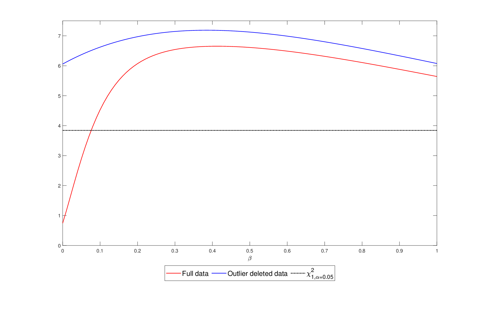
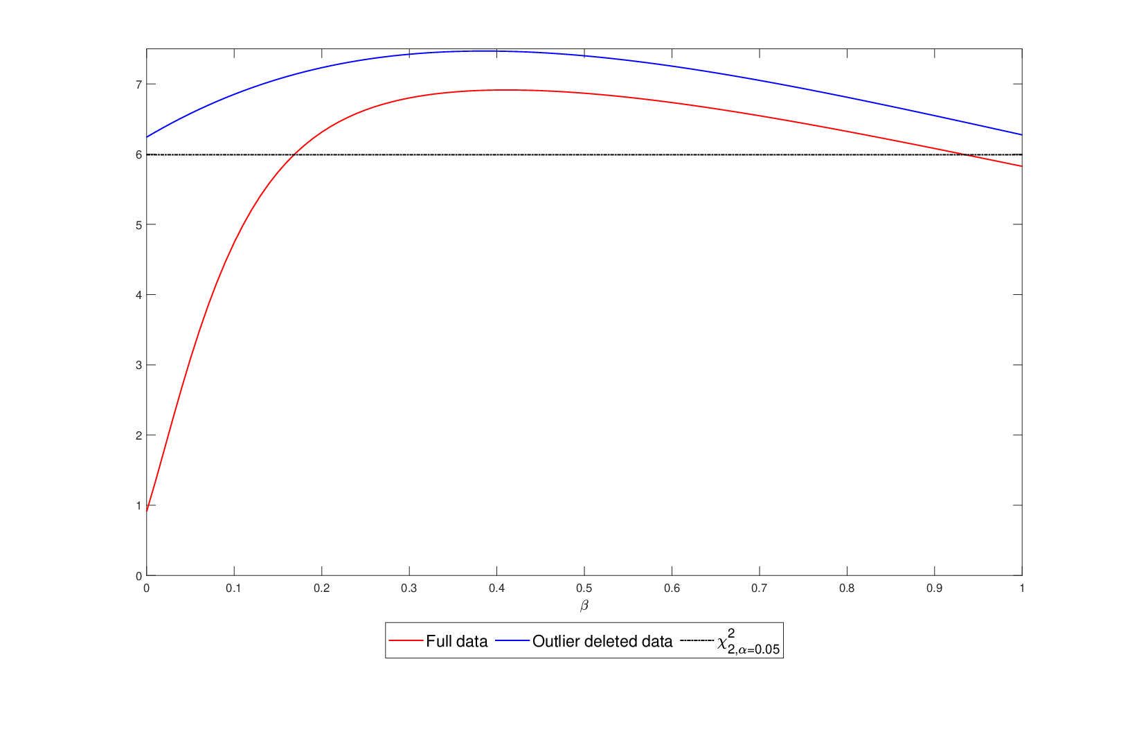
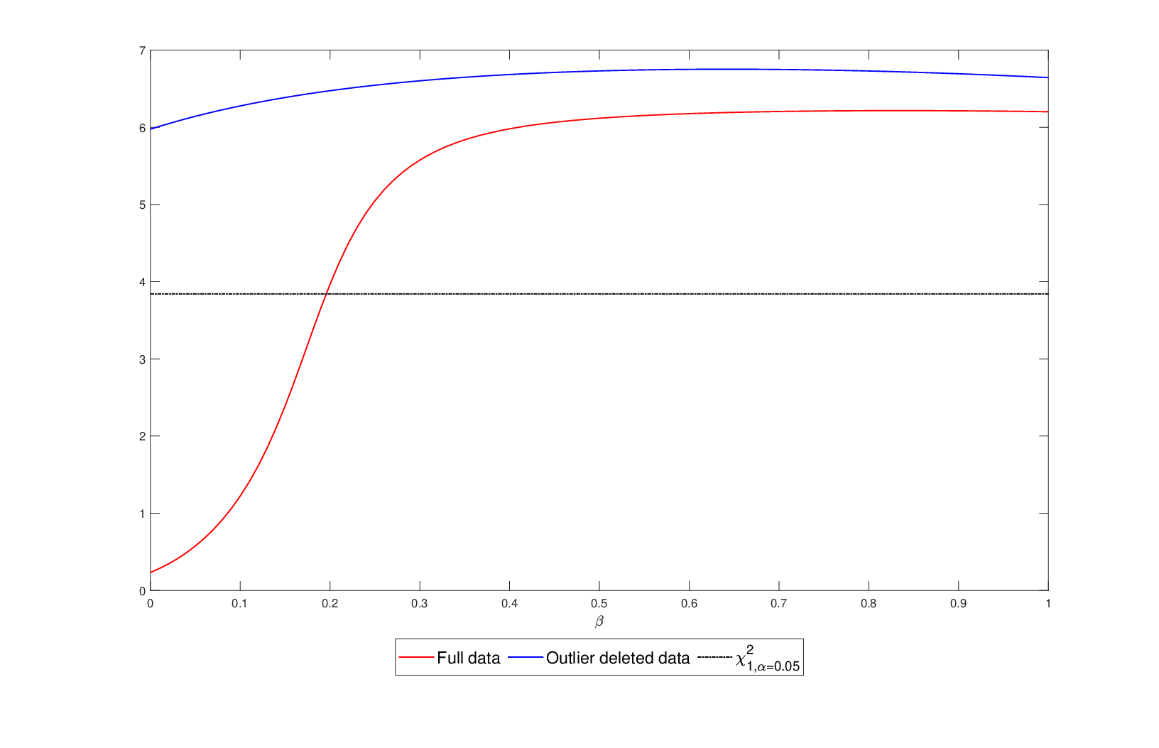
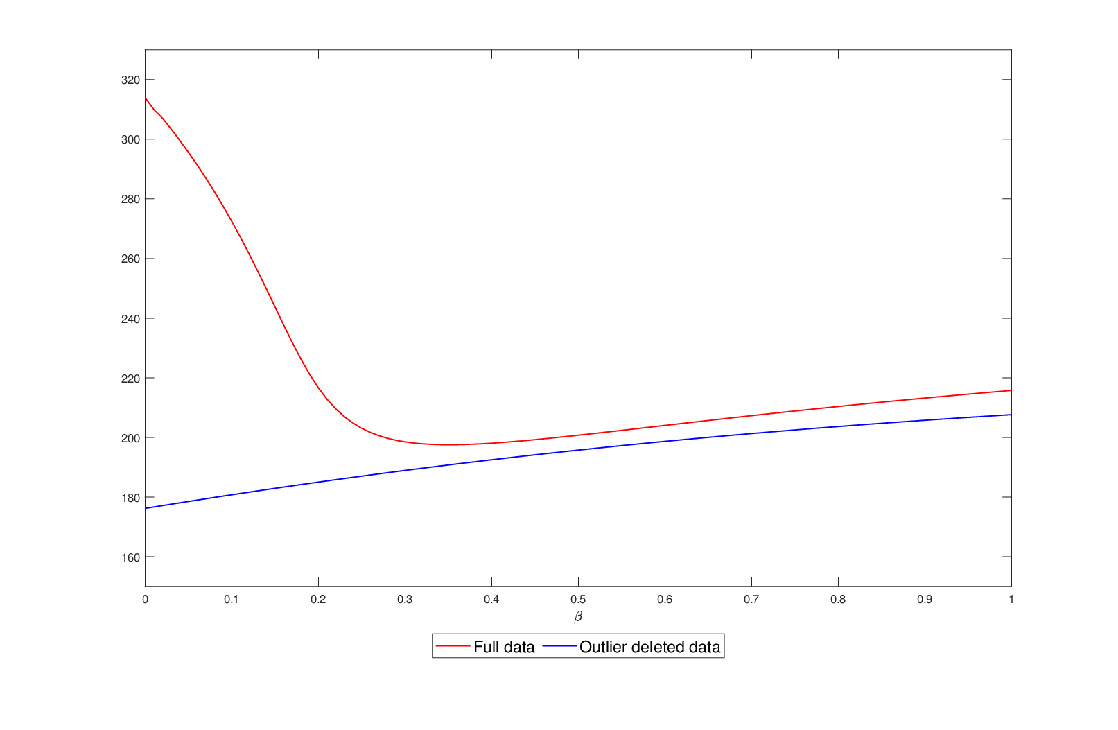
We consider the data on telephone line faults analyzed, among others, in Basu et al. (2013). The data are presented in Table 1 and consist of the ordered differences between the inverse test rates and the inverse control rates in matched pairs of areas. The first observation of this dataset is a huge outlier with respect to the normal model. In the following three subsections three different hypothesis testing problems are considered to be analyzed with this data set.

pairs	$1$	$2$	$3$	$4$	$5$	$6$	$7$	$8$	$9$	$10$	$11$	$12$	$13$	$14$
differences	$-988$	$-135$	$-78$	$3$	$59$	$83$	$93$	$110$	$189$	$197$	$204$	$229$	$289$	$310$

Table 1: Telephone-line faults data

6.1 Example 1 (One-dimensional simple null hypothesis)

Suppose we have an i.i.d. sample $X_{1},\ldots,X_{n}$ from a normal population with variance $\sigma_{0}^{2}$ and unknown mean $\mu$ . We want to test the hypothesis

H_{0}:\mu=\mu_{0}\text{ against }H_{1}:\mu\neq\mu_{0}

using the proposed Rao-type test statistics. In this case the full parameter space is given by $\Theta=\{\mu\in\mathbb{R}\}$ , while that under the null hypothesis is given by a unique point $\Theta_{0}=\{\mu\in\mathbb{R}:\mu=\mu_{0}\}$ . Direct calculations show that $u_{\beta}\left(X,\mu\right)$ , as defined in Equation (16) is given by

u_{\beta}\left(x,\mu\right)=\frac{x-\mu}{\sigma_{0}^{2}}\frac{1}{\left(\sqrt{2\pi}\sigma_{0}\right)^{\beta}}\exp\left(-\frac{\beta}{2}\left(\frac{x-\mu}{\sigma_{0}}\right)^{2}\right).

It is also easy to check

u(x,\mu_{0})=u_{\beta=0}\left(x,\mu_{0}\right)=\frac{x-\mu_{0}}{\sigma_{0}^{2}}~\text{and}~\xi\left(\mu_{0}\right)=\int_{-\infty}^{+\infty}u(x,\mu_{0})f_{\mu_{0}}^{\beta+1}(x)dx=0.

Also

	$\displaystyle K_{\beta}\left(\mu_{0}\right)$	$\displaystyle=\int_{-\infty}^{+\infty}u^{2}\left(x,\mu\right)f_{\mu_{0}}^{2\beta+1}(x)dx-\xi^{2}\left(\mu_{0}\right).$
		$\displaystyle=\int_{-\infty}^{+\infty}\left(\frac{x-\mu_{0}}{\sigma_{0}^{2}}\right)^{2}\frac{1}{\left(\sqrt{2\pi}\sigma_{0}\right)^{2\beta+1}}\exp\left(-\frac{2\beta+1}{2}\left(\frac{x-\mu_{0}}{\sigma_{0}}\right)^{2}\right)dx-0$
		$\displaystyle=\frac{1}{\left(2\pi\right)^{\beta}\sigma_{0}^{2\beta+2}\left(2\beta+1\right)^{\frac{3}{2}}}.$

Then

$\displaystyle R_{\beta,n}\left(\mu_{0}\right)$	$\displaystyle=nU_{\beta}^{2}\left(\mu\right)\left/K_{\beta}\left(\mu_{0}\right)\right.=\frac{1}{nK_{\beta}\left(\mu_{0}\right)}\left(\sum\limits_{i=1}^{n}u_{\beta}\left(X_{i},\mu\right)\right)^{2}$
	$\displaystyle=\frac{\left(2\pi\right)^{\beta}\sigma_{0}^{2\beta+2}}{n\left(2\beta+1\right)^{-\frac{3}{2}}}\left[\sum_{i=1}^{n}\frac{X_{i}-\mu_{0}}{\sigma_{0}^{\beta+2}}\frac{1}{\left(2\pi\right)^{\frac{\beta}{2}}}\exp\left(-\frac{\beta}{2}\left(\frac{X_{i}-\mu_{0}}{\sigma_{0}}\right)^{2}\right)\right]^{2}$
	$\displaystyle=\frac{\left(2\beta+1\right)^{\frac{3}{2}}}{n}\left(\sum_{i=1}^{n}\frac{X_{i}-\mu_{0}}{\sigma_{0}}\exp\left(-\frac{\beta}{2}\left(\frac{X_{i}-\mu_{0}}{\sigma_{0}}\right)^{2}\right)\right)^{2}.$	(41)

For $\beta=0$ , we recover the score equation for the MLE, and the test statistic reduces to the classical Rao statistic

R_{n}\left(\mu_{0}\right)=R_{\beta=0,n}\left(\mu_{0}\right)=\left(\frac{\bar{X}_{n}-\mu_{0}}{\frac{\sigma_{0}}{\sqrt{n}}}\right)^{2}.

where $\bar{X}_{n}$ is the sample mean.

In the top panel of Figure 1 the values of the Rao type test statistics are plotted for the telephone-line faults data for $\mu_{0}=0$ and $\sigma_{0}=175$ . The threshold for the acceptance region of the null hypothesis shows that for outlier deleted data, i.e. when the first observation is removed, the null hypothesis is rejected for all values of $\beta\in[0,1]$ at the nominal level $\alpha=0.05$ ; however, the full data set, the null hypothesis cannot be rejected for most values of $\beta<0.1$ , including for the classical Rao test-statistic ( $\beta=0$ ). The difference in the final conclusion of the test in the full data and outlier deleted data scenarios indicate the lack of robustness of the classical Rao statistic, in that here a single extreme observation is able to control the conclusion of the test in a sample of size $14$ . On the other hand, values of $\beta>0.1$ lead to a similar conclusion for the Rao type test statistic with or without outlier; this indicates the outlier stability of the proposed Rao type test statistics for moderately large values of $\beta$ .

Refer to caption — Figure 1: Telephone-line faults data: $R_{n,\beta}(\mu_{0})$ in the top and $R_{n,\beta}(\mu_{0},\sigma_{0})$ in the bottom, both in terms of tuning parameter $\beta$ on abscissa axis

6.2 Example 2 (Two-dimensional simple null hypothesis)

Let $X$ be a normal population with both parameters $\mu$ and $\sigma$ unknown. We want to derive the Rao-type test statistics for testing

H_{0}:\left(\mu,\sigma\right)=\left(\mu_{0},\sigma_{0}\right)\text{ against }H_{1}:\left(\mu,\sigma\right)\neq\left(\mu_{0},\sigma_{0}\right).

(42)

In this case the full parameter space is given by $\Theta=\{\left(\mu,\sigma\right)\in\mathbb{R}\times\mathbb{R}^{+}\}$ , while that under the null hypothesis is given by a unique point $\Theta_{0}=\{\left(\mu,\sigma\right)\in\mathbb{R}\times\mathbb{R}^{+}:(\mu,\sigma)=(\mu_{0},\sigma_{0})\}$ . In order to evaluate $\boldsymbol{u}_{\beta}\left(x,\mu_{0},\sigma_{0}\right)=\left(u_{\beta,1}\left(x,\mu_{0},\sigma_{0}\right),u_{\beta,2}\left(x,\mu_{0},\sigma_{0}\right)\right)^{T}$ , note that from the previous example we have

u_{\beta,1}\left(x,\mu,\sigma\right)=\frac{x-\mu}{\sigma^{\beta+2}}\frac{1}{\left(2\pi\right)^{\frac{\beta}{2}}}\exp\left(-\frac{\beta}{2}\left(\frac{x-\mu}{\sigma}\right)^{2}\right).

(43)

Simple calculations yield

u_{\beta,2}\left(x,\mu,\sigma\right)=\frac{1}{\sigma^{\beta+1}\left(2\pi\right)^{\beta/2}}\left[\left(\frac{(x-\mu)^{2}}{\sigma^{2}}-1\right)\exp\left(-\frac{\beta}{2}\left(\frac{x-\mu}{\sigma}\right)^{2}\right)+\frac{\beta}{\left(\beta+1\right)^{3/2}}\right],

(44)

and

$\displaystyle\boldsymbol{K}_{\beta}\left(\mu,\sigma\right)$	$\displaystyle=\mathrm{diag}\{K_{\beta,11}(\mu,\sigma),K_{\beta,22}(\mu,\sigma)\},$	(45)
$\displaystyle K_{\beta,11}(\mu,\sigma)$	$\displaystyle=\frac{1}{\sigma^{2(\beta+1)}\left(2\pi\right)^{\beta}\left(2\beta+1\right)^{3/2}},$
$\displaystyle K_{\beta,22}(\mu,\sigma)$	$\displaystyle=\frac{\tau(\beta)}{\sigma^{2(\beta+1)}\left(2\pi\right)^{\beta}},$
$\displaystyle\tau(\beta)$	$\displaystyle=\frac{2\left(2\beta^{2}+1\right)\sqrt{2\beta+1}}{(2\beta+1)^{3}}-\frac{\beta^{2}}{(\beta+1)^{3}},$	(46)

Making use of the above, the Rao-type test statistics finally turns out to be

	$\displaystyle R_{\beta,n}\left(\mu_{0},\sigma_{0}\right)$	$\displaystyle=R_{\beta,n}\left(\mu_{0}\right)+R_{\beta,n}\left(\sigma_{0}\right),$
	$\displaystyle R_{\beta,n}\left(\mu_{0}\right)$	$\displaystyle=\frac{1}{nK_{\beta,11}(\mu_{0},\sigma_{0})}\left(\sum_{i=1}^{n}u_{\beta,1}\left(X_{i},\mu_{0},\sigma_{0}\right)\right)^{2},$
	$\displaystyle R_{\beta,n}\left(\sigma_{0}\right)$	$\displaystyle=\frac{1}{nK_{\beta,22}(\mu_{0},\sigma_{0})}\left(\sum_{i=1}^{n}u_{\beta,2}\left(X_{i},\mu_{0},\sigma_{0}\right)\right)^{2},$

the combination of two one-dimensional Rao-type test statistics. On one hand, $R_{\beta,n}\left(\mu_{0}\right)$ has the same expression as (41), and is useful to test the hypothesis

H_{0}:\mu=\mu_{0}\text{ against }H_{1}:\mu\neq\mu_{0}

from a normal population with known variance $\sigma_{0}^{2}$ and unknown mean $\mu$ . On the other hand

R_{\beta,n}\left(\sigma_{0}\right)=\frac{1}{n\tau(\beta)}\left(\sum_{i=1}^{n}\left[\left(\frac{X_{i}-\mu_{0}}{\sigma_{0}}\right)^{2}-1\right]\exp\left(-\frac{\beta}{2}\left(\frac{X_{i}-\mu_{0}}{\sigma_{0}}\right)^{2}\right)+\frac{\beta}{\left(\beta+1\right)^{3/2}}\right)^{2},

with $\tau(\beta)$ given by (46), has the same expression as the Rao type test statistics to test the hypothesis

H_{0}:\sigma^{2}=\sigma_{0}^{2}\text{ against }H_{1}:\sigma^{2}\neq\sigma_{0}^{2}

from a normal population with known mean $\mu_{0}$ and unknown variance $\sigma^{2}$ . For $\beta=0$ , we get

	$\displaystyle R_{\beta=0,n}\left(\mu_{0}\right)$	$\displaystyle=\left(\frac{\bar{X}_{n}-\mu_{0}}{\frac{\sigma_{0}}{\sqrt{n}}}\right)^{2},~R_{\beta=0,n}\left(\sigma_{0}\right)=\frac{n}{2}\left(\frac{S_{\mu_{0}}^{2}-\sigma_{0}^{2}}{\sigma_{0}^{2}}\right)^{2},$
	$\displaystyle S_{\mu_{0}}^{2}$	$\displaystyle=\frac{1}{n}\sum_{i=1}^{n}\left(X_{i}-\mu_{0}\right)^{2},$		(47)

so that the classical Rao test for testing the hypothesis (42) is given by the statistic

R_{\beta=0,n}\left(\mu_{0},\sigma_{0}\right)=\left(\frac{\bar{X}_{n}-\mu_{0}}{\frac{\sigma_{0}}{\sqrt{n}}}\right)^{2}+\frac{n}{2}\left(\frac{S_{\mu_{0}}^{2}-\sigma_{0}^{2}}{\sigma_{0}^{2}}\right)^{2},

which is the classical Rao test for this hypothesis $R_{n}\left(\mu_{0},\sigma_{0}\right)$ .

In the bottom panel of Figure 1 the value of Rao type test statistics is plotted for telephone-line faults data for $\mu_{0}=0$ and $\sigma_{0}=175$ . The threshold for the acceptance region of the null hypothesis shows that for outlier deleted data, i.e. when the first observation is removed, the null hypothesis cannot be rejected with $\alpha=0.05$ , however for most of values $\beta<0.2$ , including the classical Rao test statistic ( $\beta=0$ ), the null hypothesis is rejected for the full data set. This different conclusion in the decision of the test clarifies the lack of robustness of the classical Rao test statistic. On the other hand, most of values $\beta>0.2$ have a similar value of the Rao type test statistic deleting or not the outlier, this fact shows the robust property of the proposed Rao type test statistics.

6.3 Example 3 (Two-dimensional composite null hypothesis)

Let $X$ be a normal population with unknown variance $\sigma^{2}$ and mean $\mu.$ We will develop the Rao-type test statistics for testing

H_{0}:\mu=\mu_{0}\text{ against }H_{1}:\mu\neq\mu_{0},

where $\sigma^{2}$ is an unknown nuisance parameter. In this case the full parameter space is given by $\Theta=\{\left(\mu,\sigma\right)\in\mathbb{R}\times\mathbb{R}^{+}\}$ , while that under the null hypothesis is given by $\Theta_{0}=\{\left(\mu,\sigma\right)\in\mathbb{R}\times\mathbb{R}^{+}:\mu=\mu_{0}\}$ , which is fixed in one of the two dimensions. If we consider the function $m\left(\mu,\sigma\right)=\mu-\mu_{0},$ the null hypothesis $H_{0}$ can be written alternatively as

H_{0}:m(\mu,\sigma)=0.

We can observe that in our case $\boldsymbol{M}\left(\mu,\sigma\right)=\left(1,0\right)^{T}$ . With $f_{\mu_{0},\sigma^{2}}(x)$ being the normal density with mean $\mu_{0}$ and variance $\sigma^{2}$ , we consider the statistic given in Equation (33), with $r=1$ and $\boldsymbol{K}_{\beta}\left(\mu,\sigma\right)$ given by (45). On the other hand

\boldsymbol{U}_{\beta,n}(\mu_{0},\widetilde{\sigma}_{\beta})=\frac{1}{n}\left(\sum_{i=1}^{n}u_{\beta,1}\left(X_{i},\mu_{0},\widetilde{\sigma}_{\beta}\right),\sum_{i=1}^{n}u_{\beta,2}\left(X_{i},\mu_{0},\widetilde{\sigma}_{\beta}\right)\right)^{T},

with $u_{\beta,1}\left(x,\mu,\sigma\right)$ and $u_{\beta,2}\left(x,\mu,\sigma\right)$ being as given in Equations (43) and (44), respectively. The estimator $\boldsymbol{\tilde{\theta}}_{\beta}=\left(\mu_{0},\widetilde{\sigma}_{\beta}\right)^{T}$ , for known $\mu=\mu_{0}$ when $\beta>0$ , is the solution of the nonlinear equation $U_{2,\beta,n}(\mu_{0},\widetilde{\sigma}_{\beta})=0$ , with $u_{2,\beta}\left(x,\mu,\sigma\right)$ given $\mu=\mu_{0}$ has the same expression as (44) and $U_{2,\beta,n}(\mu_{0},\widetilde{\sigma}_{\beta})=\frac{1}{n}\sum_{i=1}^{n}u_{2,\beta}\left(X_{i},\mu_{0},\sigma\right)$ . Based on the previous calculations, we have

	$\displaystyle\tilde{R}_{\beta,n}(\mu_{0},\widetilde{\sigma}_{\beta})$	$\displaystyle=\frac{1}{n}K_{\beta,11}(\mu_{0},\widetilde{\sigma}_{\beta})\left(\sum_{i=1}^{n}u_{\beta,1}\left(X_{i},\mu_{0},\widetilde{\sigma}_{\beta}\right)\right)^{2}$
		$\displaystyle=\frac{1}{n}\left(2\beta+1\right)^{\frac{3}{2}}\left(\sum_{i=1}^{n}\frac{X_{i}-\mu_{0}}{\widetilde{\sigma}_{\beta}}\exp\left(-\frac{\beta}{2}\left(\frac{X_{i}-\mu_{0}}{\widetilde{\sigma}_{\beta}}\right)^{2}\right)\right)^{2}.$

In particular, since $\widetilde{\sigma}_{\beta=0}^{2}=S_{\mu_{0}}^{2}$ given by (47) for $\beta=0$ , the classical Rao test statistic has the following simple expression

\tilde{R}_{n}(\mu_{0},S_{\mu_{0}}^{2})=\tilde{R}_{\beta=0,n}(\mu_{0},\widetilde{\sigma}_{\beta=0})=\left(\frac{\bar{X}_{n}-\mu_{0}}{\frac{S_{\mu_{0}}}{\sqrt{n}}}\right)^{2}.

In the top panel of Figure 2 the values of the Rao type test statistics are plotted for the telephone-line faults data for $\mu_{0}=0$ . For the cleaned data, i.e., with the first observation removed, all Rao-type test statistics are above the threshold and are able to reject the null hypothesis at the nominal level $\alpha=0.05$ . However, for the full data, most values of $\beta<0.2$ produce test statistics smaller than the threshold and therefore fail to reject the null hypothesis. The closeness of the statistics for the full data and the outlier deleted data as a function of $\beta$ correspond approximately to the closeness of the scale estimates for the full data and the outlier deleted data which is demonstrated in the bottom panel of Figure 2. On the whole this gives a good illustration of the robustness and stability properties of the Rao-type test statistics for larger values of $\beta$ .

7 Simulation study

We have considered the one-dimensional simple null hypothesis and the two-dimesnional composite null hypothesis for studying the performance of the Rao-type test statistics for normal populations. Our simulations have covered eleven values of the tuning parameter $\beta=k\times 0.1$ for $k\in\{0,1,...,10\}$ ; however in our plots we have only included seven values associated to $k\in\{0,2,...,10\}\cup\{3\}$ to make the identification of different curves, associated with $\beta$ , easier. We have used $R=1,000,000$ replications and have taken sample sizes equal to $n\in\{5,6,...,50\}$ ; when $10\%$ contamination is introduced, some of the smaller samples may not have any outliers at all, but by the time samples are of sizes around $50$ , and reasonable stability in the general behavior of the Rao-type test statistics under contamination should be observable under the two scenarios we are going to describe.

Scenario 1: This is based on Example 6.1 (one-dimensional simple null hypothesis). Here $X$ is assumed to be a normal random variable with known variance $\sigma_{0}^{2}=1$ and unknown mean $\mu$ . The corresponding Rao-type test statistics for testing

H_{0}:\mu=0\text{ against }H_{1}:\mu\neq 0,

(48)

is given by

R_{\beta,n}\left(\mu_{0}=0\right)=\frac{1}{n}\left(2\beta+1\right)^{\frac{3}{2}}\left(\sum_{i=1}^{n}X_{i}\exp\left(-\frac{\beta}{2}X_{i}^{2}\right)\right)^{2}.

The empirical significance level of this test (at nominal level $\alpha$ ) is computed as the proportion of replications (out of the total $R$ ) where the Rao-type test statistic exceeds the asymptotic threshold given by $\chi_{1,\alpha}^{2}$ ( $\chi_{1}^{2}$ quantile of order $\alpha$ , on the right), with $\alpha=0.05$ . For pure data it is seen, at the top panel of Figure 3, that the quantile of the classical Rao test statistic ( $\beta=0$ ) matches almost perfectly with the chi-square quantile of order $0.05$ for any sample size $n$ , and the variation around the line $\alpha=0.05$ is due to the sampling fluctuations (smaller than $1\%$ in absolute value) alone. As $n$ increases, the empirical levels of the Rao-type test statistics (for all $\beta$ ) get closer to the nominal values. The approximation is better as $\beta$ is closer to $0$ , and hence $\beta=0.2$ has better performance than $\beta=0.4$ , but worse than $\beta=0$ , in overall terms for all sample sizes.

In order to study attained levels of our proposed tests the performance of the significance levels under contamination, we generated observations from the $0.9\mathcal{N}(0,1)+0.1\mathcal{N}(-4.5,1)$ mixture. It is observed that all test statistics corresponding to $\beta\geq 0.4$ provide remarkably stable results in terms of the closeness to the empirical levels and nominal levels. For very small values of $\beta$ the results are generally reasonable at small sample sizes; however for $n>10$ , the empirical level of the classical Rao test blows up with increasing sample size. The same phenomenon is observed, at a lesser degree, for the test corresponding to $\beta=0.2$ . A slow inflation appears to take place for $\beta=0.3$ as well.

To investigate the power behavior of the Rao-type test statistics under pure data, we have taken $\mathcal{N}(-0.5,1)$ for all simulations; the empirical power of a given test is the empirical proportion of the number of test statistics exceeding the chi-square quantile threshold, $\chi_{1,\alpha}^{2}$ . As shown in the top panel of Figure 4, the classical Rao test statistic ( $\beta=0$ ) exhibits the highest power with pure data and in general as $\beta$ decreases the power is higher. For creating contamination, the samples for the scenario described in the bottom panel of Figure 4 come from the normal mixture $0.9\mathcal{N}(-0.5,1)+0.1\mathcal{N}(5,1)$ . Under contaminated data the classical Rao test statistic ( $\beta=0$ ) exhibits a very significant drop in power, making the power curve practically flat. Most of the test statistics corresponding to positive values of $\beta$ perform much better in holding the power levels under contamination. The best performance in terms of power under contamination is provided by the test-statistic corresponding to $\beta=0.4$ .

Scenario 2: Taking Example 6.3 as the basis (two-dimensional composite null hypothesis), we have taken $X$ to be a normally distributed random variable with unknown mean $\mu$ and variance $\sigma^{2}$ . The corresponding Rao-type test statistics for testing the hypothesis in (48) is given by

\tilde{R}_{\beta,n}\left(\mu_{0}=0,\widetilde{\sigma}_{\beta}^{2}\right)=\frac{1}{n}\left(2\beta+1\right)^{\frac{3}{2}}\frac{1}{\widetilde{\sigma}_{\beta}^{2}}\left(\sum_{i=1}^{n}X_{i}\exp\left(-\frac{\beta}{2}\frac{X_{i}^{2}}{\widetilde{\sigma}_{\beta}^{2}}\right)\right)^{2},

where $\widetilde{\sigma}_{\beta}^{2}$ is the estimation of $\sigma^{2}$ under the assumption that $\mu_{0}=0$ . The scheme of contamination and outliers is exactly the same as for Scenario 1, but the results shown in Scenario 2, by Figures 5-6, are very different. Surprisingly, for pure data the ordinary Rao test is conservative, particularly in small samples, and the nominal levels are better approximated with $\beta>0.2$ than for $\beta=0$ , and under contamination the ordinary Rao test simply breaks down, while all the others reasonably hold their level; even the $\beta=0.2$ test has an observed level less than 0.1 at a sample size of $n=50$ (Figure 5). Power calculations for pure data indicate that the ordinary Rao test has high power except at very low sample sizes (a consequence of its conservative nature), but its power practically vanishes under contamination, where values of $\beta$ between 0.6 and 0.8 appear to have the best performance (Figure 6).

8 Concluding Remarks

The traditional Rao test is a very useful tool in applied statistics and econometrics. However, as the default application of tests of this type are based the maximum likelihood estimator and the likelihood score function, lack of robustness and sensitivity to outliers is an inherent problem in the traditional Rao test. In this paper we have proposed a c;lass of Rao type tests, including the ordinary Rao test, many members of which have remarkable robustness properties often with very little loss in power relative to the ordinary Rao test. In i.i.d. data the application of the test is simple, and we believe that the theoretical results and the numerical support demonstrate that the class of tests help to cover the primary deficiency of the traditional Rao test at a very little cost.

References

[1] Aitchison, J. and Silvey, S. D. (1958). Maximum likelihood estimation of parameters subject to restraints. Annals of Mathematical Statistics, 29, 813-828.
[2] Basu, A., Harris, I. R., Hjort, N. L. and Jones, M. C. (1998). Robust and efficient estimation by minimizing a density power divergence. Biometrika, 85, 549–559.
[3] Basu, A., Mandal, A., Martin, N. and Pardo, L. (2013). Testing statistical hypotheses based on the density power divergence. Annals of the Institute of Statistical Mathematics, 65, 319–348.
[4] Basu, A., Mandal, A., Martin, N. and Pardo, L. (2016). Generalized Wald-type tests based on minimum density power divergence estimators. Statistics, 50, 1–26.
[5] Basu, A., Shioya, H. and Park, C. (2011). Statistical Inference: The Minimum Distance Approach. CRC Press, Boca Raton, Florida.
[6] Bera, A.K. and MacKenzie, C.R. (1986). Alternative forms and properties of the score test. Journal of Applied Statistics, 13,13–25.
[7] Bera, A.K. and Ullah, A. (1991). Rao’s score test in econometrics. Journal of Quantitative Economics, 7, 189–220.
[8] Breusch, T.S. and Pagan, A.R. (1980). The Lagrange multiplier test and its application to model specification in econometrics. The Review of Economic Studies, 47, 239–253.
[9] Chandra, T. K. and Joshi, S. N. (1983). Comparison of the likelihood ratio, Rao’s and Wald’s tests and a conjecture of C. R. Rao. Sankhya, A, 45 226–246.
[10] Chandra, T. K. and Mukerjee, R. (1985). On the optimahty of Rao’s statistic. Communications in Statistics (Theory and Methods), 13 1507-1515.
[11] De Angelis, D. and G. A. Young (1992). Smoothing the bootstrap. International Statistical Review, 60, 45–56.
[12] Engle, R.F. (1984). Wald, likelihood ratio and Lagrange multiplier tests in econometrics. In: Griliches, Z., Intriligator, M.D. (Eds.), Handbook of Econometrics, Vol. 2. North-Holland, Amsterdam, 775–826.
[13] Godfrey, L.G. (1988). Misspecification Tests in Econometrics. Cambridge University Press, Cambridge.
[14] Godfrey, L.G. (1996). Misspecication tests and their uses in econometrics. Journal of Statistical Planning and Inference, 49, 241–260.
[15] Godfrey, L.G. and Orme, C.D. (2001). On improving the robustness and reliability of Rao’s score test. Journal of Statistical Planning and Inference, 97, 153-176.
[16] Godfrey, L. G. and Tremayne, R. (1988). Checks of Model adequacy for univariate time series models and their applications to Econometrics relationships. Econometric Reviews, 7, 1-42.
[17] Ghosh, A., Mandal, A., Martin, N. and Pardo, L. (2016). Influence Analysis of Robust Wald-type Tests. Journal of Multivariate Analysis, 147, 102–126.
[18] Kotz, S., Johnson, N. L. and Boyd, D. W. (1967b). Series representations of distributions of quadratic forms in normal variables. II. Non-central case. Annals of Mathematical Statistics, 38, 838–848.
[19] Kramer, W., Sonnberger, H. (1986). The Linear Regression Model under Test. Physica Verlag, Heidelberg.
[20] Li, Bing (2001). Sensitivity of Rao’s score test, the Wald test and the likelihood ratio test to nuisance parameters, Journal of Statistical Planning and Inference, 97, 57-66.
[21] Maddala, G.S. (1995). Specification tests in limited dependent variables. In: Maddala, G.S., Phillips, P.C.B., Srinivasan, T.N. (Eds.), Advances in Econometrics and Quantitative Economics: Essays in Honor of C.R. Rao. Blackwell, Oxford, 1–49.
[22] Mukerjee, R. (1993). Rao’s score test: recent asymptotic results. In: Maddala, G.S., Rao, C.R., Vinod, H.D. (Eds.), Handbook of Statistics, Vol. 11. North-Holland, Amsterdam.
[23] Neyman, J. and Pearson, E. S. (1928). On the use and interpretation of certain test criteria for purposes of statistical Inference. Biometrika, 20, 175-240.
[24] Neyman, J. and Pearson, E. S. (1933). On the Problem of the Most Efficient Tests of Statistical Hypotheses. Philosophical Transactions of the Royal Society of London. Series A, Containing Papers of a Mathematical or Physical Character. 231, 289-337.
[25] Pearson, K. (1900). On the criterion that a given system of deviations from the probable in the case of a correlated system of variables is such that it can be reasonably supposed to have arisen from random sampling. Philosophical Magazine, 5, 157–175.
[26] Peers, H. W. (1971). Likelihood ratio and associated test criteria, Biometrika, 58, 577-487.
[27] Rao, C. R. (1948). Large sample tests of statistical hypotheses concerning several parameters with application to problems of estimation. Proceedings of the Cambrigde Philosophical Society, 44, 50–77.
[28] Rao, C. R. (1973). Linear statistical inference and its applications. Wiley (Second Edition), New York.
[29] Rao, C. R. (2005). Score test: Historical Review and Recent Developments. In Balakrishnan, N., Kannan, N. and Nagaraja, H. N. (Eds.), Advances in Ranking and Selection, Multiple Comparisons and Reliability Statistics for Industry and Technology, pp. 3-20. Birkhäuser.
[30] Silvey, S. D. (1959). The Lagrangian multiplier test, Annals of Mathematical Statistics, 30, 389–407.
[31] van der Vaart, A. W. (1990). Asymptotic Statistics. Cambridge University Press, New York.
[32] Wald, A. (1943). Tests of statistical hypothesies concerning several parameters when the number of observations is large. Transactions of the American Mathematical Society, 54, 426–482.
[33] White, H. (1984). Asymptotic Theory for Econometrics. Academic Press, New York.