Multi-Task Deep Learning with Dynamic Programming for Embryo Early Development Stage Classification from Time-Lapse Videos
Abstract
Time-lapse is a technology used to record the development of embryos during in-vitro fertilization (IVF). Accurate classification of embryo early development stages can provide embryologists valuable information for assessing the embryo quality, and hence is critical to the success of IVF. This paper proposes a multi-task deep learning with dynamic programming (MTDL-DP) approach for this purpose. It first uses MTDL to pre-classify each frame in the time-lapse video to an embryo development stage, and then DP to optimize the stage sequence so that the stage number is monotonically non-decreasing, which usually holds in practice. Different MTDL frameworks, e.g., one-to-many, many-to-one, and many-to-many, are investigated. It is shown that the one-to-many MTDL framework achieved the best compromise between performance and computational cost. To our knowledge, this is the first study that applies MTDL to embryo early development stage classification from time-lapse videos.
Index Terms:
Multi-task learning, in-vitro fertilization, convolutional neural networks, dynamic programming, image classificationI Introduction
In-vitro fertilization (IVF) [1, 2, 3] is a frequently used technology for treating infertility. The process involves the collection of multiple follicles for fertilization and in-vitro culture. Cultivation, selection and transplantation of embryo are the key steps in determining a successful implantation during IVF [4, 5]. During the development of embryos, the morphological characteristics [6] and kinetic characteristics [7] are highly correlated with the outcome of transplantation.
Time-lapse videos have been widely used in various reproductive medicine centers during the cultivation of embryos [8] to monitor them. A time-lapse video records the embryonic development process in real time by taking photos of the embryos at short time intervals [9]. Thus, a large amount of time series image data for each embryo are produced in this process. At the final stage of embryo selection, an embryologist reviews the entire embryo development process to score and sort them. Studies with different time-lapse equipment reported improved prediction accuracy of embryo implantation potential by analyzing the morphokinetics of human embryos at early cleavage stages [9, 10, 11, 8, 12]. These features have been shown to be statistically significant to the final outcome of the transplantation [7].
There have been only a few approaches to analyze time-lapse image data [9, 13, 14, 15, 16, 17, 18]. Due to the limitations of the time-lapse technology, stereoscopic cells of different heights overlap in the images when photographed. It is difficult for even an experienced embryologist to accurately count the number of cells in a single time-lapse image when there are more than eight cells. Therefore, most research focused on the early development stages of embryos. Wong et al. [9] identified several key parameters that can predict blastocyst formation at the 4-cell stage from time-lapse images, and employed sequential Monte Carlo based probabilistic model estimation to monitor these parameters and track the cells. Wang et al. [13] presented a multi-level embryo stage classification approach, by using both hand-crafted and automatically learned embryo features to identify the number of cells in a time-lapse video. Conaghan et al. [14] used an automated and proprietary image analysis software EEVATM (Early Embryo Viability Assessment), which exhibited high image contrast through the use of darkfield illumination, to track cell divisions from one-cell stage to four-cell stage. Their experiments verified that the EEVA Test can significantly improve embryologists’ ability to identify embryos that would develop into usable blastocysts. There are also several other studies on embryo selection by using EEVATM [19, 20, 21, 22], but they did not provide the details of the used EEVA Test. Jonaitis et al. [15] compared the performance of neural network, support vector machine and nearest neighbor classifier in detecting cell division time. Khan et al. [18] used a deep convolutional neural network (CNN) to classify the number of cells, and also semantic segmentation to extract the cell regions in a time-lapse image [16]. Ng et al. [17] combined late fusion networks with dynamic programming (DP) to predict different cell development stages and obtained better results than a single-frame model.
Multi-task learning has been successfully used in many applications, such as natural language processing [23], speech recognition [24], and computer vision [25]. Its basic idea is to share representations among related tasks, so that each trained model may have better generalization ability [26]. This paper proposes a multi-task deep learning with dynamic programming (MTDL-DP) approach, which first uses MTDL to pre-classify each frame in the time-lapse video to an embryo development stage, and then DP to optimize the stage sequence so that the stage number is monotonically non-decreasing, which usually holds in practice. To our knowledge, this is the first study that applies MTDL to embryo early development stage classification from time-lapse videos.
II Classification Frameworks
This section introduces four frameworks for embryo early development stage classification from time-lapse videos. We first describe our dataset and the baseline network architecture, and then extend it to many-to-one, one-to-many and many-to-many MTDL frameworks.
II-A Dataset
The time-lapse video dataset used in our experiments came from the Reproductive Medicine Center of Tongji Hospital, Huazhong University of Science and Technology, Wuhan, China. It consisted of 170 time-lapse videos extracted from incubators, using an EmbryoScope+ time-lapse microscope system11 1 https://www.vitrolife.com/products/time-lapse-systems/embryoscopeplus-time-lapse-system/ at 10-minute sampling interval. Each frame in the video is a grayscale image with a well number in the lower left corner and a time marker after fertilization in the lower right corner, as shown in Fig. 1. The embryo is surrounded by some granulosa cells in the microscope field. The scale bar in the upper right corner indicates the size of the cells. Each video began about 0-2 hours after fertilization, and ended about 140 hours after fertilization. We only used the first frames in each video, which were manually labeled for the embryo development stages. Therefore, we had a total of labeled frames in the experiment.


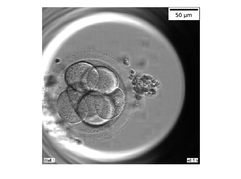
As in [17], we focused on the first six embryo development stages, which included initialization (tStart), the appearance and breakdown of the male and female pronucleus (tPNf), and the appearance of 2 through 4+ cells (t2, t3, t4, t4+). We counted the number of images in different embryo development stages in the dataset, and show the summary in Fig. 2. Note that t3 was rarely observed in our dataset.

II-B The Baseline One-to-One Classification Framework
Let be the th frame in a time-lapse video. For image classification, a standard one-to-one classification framework learns a mapping:
| (1) |
where is the stage label of , and the label set of the embryo development stages.
When information of the previous and future frames is used, the standard one-to-one classification framework can be extended to many-to-one, one-to-many and many-to-many MTDL frameworks, as illustrated in Fig. 3.


We used ResNet [27], which won the 2015 ImageNet classification competition, to process individual video frames. Table I shows our baseline ResNet50 model. The input image had three channels (RGB), each with 224224 pixels (the 800800 images were resized). The model was initialized from the ResNet weights pre-trained on ImageNet [28], which can help reduce overfitting on small datasets.
| layer name | 50-layer | output size |
| conv1 | , 64, stride | |
| res2 | max pool, stride | |
| res3 | ||
| res4 | ||
| res5 | ||
| global average pool | ||
| fc | ||
| softmax | ||
II-C The Many-to-One MTDL Framework
The many-to-one MTDL framework, shown in Fig. 3, is frequently used in video understanding [29, 30, 31] because multiple frames in the same video usually have the same label, and hence they can be considered together to predict the final label. Many-to-one can better make use of input context information than one-to-one.
Many-to-one performs the following mapping:
| (2) |
where is the number of neighboring frames before and after the current frame (the input context window size is hence ).
There are two common approaches to fuse time domain information from the frames: Conv Pooling [32] and Late Fusion [30].
II-C1 Conv Pooling
This is a convolutional temporal feature pooling architecture, which has been extensively used for video classification, especially for bag-of-words representations [33]. Image features are computed for each frame and then max pooled. The pooling features can then be sent to fully connected layers for final classification. A major advantage of this approach is that spatial information in multiple frames, output by the convolutional layers, is preserved through a max pooling operation in the time domain. Experiments [32] verified that Conv Pooling outperformed all other feature pooling approaches on the Sports-1M dataset, using a 120-frame AlexNet model [34].
II-C2 Late Fusion
In Late Fusion, all frames in the input context window are encoded via identical ConvNets. The final representations after all convolutional layers are concatenated and passed through a fully-connected layer to generate classifications. The concatenation can happen to a subset of frames in the input context window [30], or to all frames in that window [17]. Previous research [17] demonstrated that Late Fusion ConvNets using 15 frames and a DP-based decoder outperformed Early Fusion for predicting embryo morphokinetics in time-lapse videos.
II-D The One-to-Many MTDL Framework
One-to-many, shown in Fig. 3, means each input is mapped to multiple outputs, which is also called multi-task nets [35] in deep learning. This paper uses hard parameter sharing of hidden layers [26], as illustrated in Fig. 4. The parameters of the convolution layers are shared among different tasks, but those of the fully connected layers are trained separately.

In one-to-many, each is used in classifying stages centered at , i.e., it learns the following one-to-many mapping:
| (3) |
’s classification for the stage at time index is a probability vector .
At each Frame Index , the corresponding label is estimated by neighboring , . We need to aggregate them to obtain the final classification. This can be done by an ensemble approach.
Because each frame is involved in outputs, the total loss on a training frame is computed as the sum of the loss on all involved outputs:
| (4) |
where is the weight for the -th output, and is the true label for Frame . and the cross-entropy loss were used in this paper. The cross-entropy loss on the -th output can be written as follows:
| (5) |
where is the -th element of .
II-E The Many-to-Many MTDL Framework
Many-to-many can be viewed as a combination of one-to-many and many-to-one. Each input frame is processed by a separate CNN. Late Fusion was used, and the parameters of the fully connected layers were also trained separately, as shown in Fig. 3.
III Multi-Task Deep Learning with Dynamic Programming (MTDL-DP)
This section introduces our proposed MTDL-DP approach.
III-A Ensemble Learning for MTDL
As mentioned in Section II-D, a multi-task net has multiple outputs. The easiest approach to get the final classification corresponding to a specific frame is to choose the middle output of the network. A more sophisticated approach is ensemble learning [36]. We consider two common probabilistic aggregation approaches in this paper: additive mean and multiplicative mean.
Let be the predicted probability vector at Frame Index , given Frame , , as illustrated in Fig. 5. The ensemble probability at Frame Index , aggregated by the additive mean, is:
| (6) |
If the multiplicative mean is used,
| (7) |
Since each is a vector, the summation in (6) and multiplication in (7) are element-wise operations.

The final classification label for Frame is obtained by probability maximization:
| (8) |
where is the -th element of .
III-B Post-processing with DP
The number of cells in the development of an embryo is almost always non-decreasing [37]. However, this is not guaranteed in the classification outputs of MTDL. We use DP to adjust the classifications so that this constraint is satisfied.
For each video, the groundtruth stages form a sequence. MTDL outputs a probability vector before likelihood maximization at Frame , where is the estimated probability that Frame is at Stage . We define as the total loss for an estimated prediction , given the model output probability matrix . The total loss is the sum of the per-frame losses , which must be optimized subject to the monotonicity constraint: .
Two common per-frame losses [17] were used. The first is negative label likelihood (LL), defined as:
| (9) |
The second is earth mover (EM) distance, defined as:
| (10) |
The final classification stage sequence can be obtained as:
| (11) | ||||
which can be easily solved by DP, as shown in Algorithm 1.
III-C MTDL-DP
Our proposed MTDL-DP consists of three steps: 1) construct a multi-task net with the one-to-many or many-to-many MTDL framework; 2) use multiplicative mean to aggregate the prediction of the multi-task net; and, 3) post-process with DP using the EM distance per-frame loss. Its pseudocode is given in Algorithm 2.
The one-to-many MTDL framework can also be replaced by the many-to-many MTDL framework.
IV Experimental Results
This section investigates the performance of our proposed MTDL-DP.
IV-A Experimental Setup
We created training/validation/test data partitions by randomly selecting 70%/10%/20% videos from the dataset, i.e., 41,650/5,950/11,900 frames, respectively. We resized each frame to 224224 so that it can be used by ResNet50, our baseline model. Random rotation and flip data augmentation was used. All MTDL frameworks were initialized by the weights trained by one-to-one (ResNet50). Then, the convolution layer parameters were frozen, and the fully connected layers were further tuned.
We used the cross-entropy loss function and Adam optimizer [38], and early stopping to reduce overfitting, in all experiments. Multiplicative mean and EM distance per-frame loss were used in the MTDL-DP. All experiments were repeated five times, and the mean results were reported.
IV-B Classification Accuracy
First, we considered MTDL only, without using DP. The classification accuracies are shown in the left panel of Table II, with (the output context window size was ). All MTDL frameworks outperformed the one-to-one framework, suggesting using neighboring input or label information in multi-task learning was indeed beneficial.
| Framework | Method | Accuracy without DP | Accuracy with DP | ||||
|---|---|---|---|---|---|---|---|
| One-to-one | ResNet50 | 83.8% | 83.8% | 83.8% | 86.1% | 86.1% | 86.1% |
| Many-to-one | Conv Pooling | 84.7% | 84.4% | 83.8% | 85.9% | 85.1% | 84.5% |
| Late Fusion | 83.9% | 84.6% | 85.1% | 86.0% | 85.2% | 85.2% | |
| One-to-many | Multi-Task Nets (ours) | 85.0% | 85.4% | 85.3% | 86.5% | 85.8% | 85.7% |
| Many-to-many | 84.6% | 85.7% | 85.8% | 86.6% | 86.5% | 86.9% | |
For the many-to-one MTDL framework, when increased, the performance of Late Fusion also increased, whereas the performance of Conv Pooling decreased. This is intuitive, because more input information was ignored in Conv Pooling when increased.
The classification accuracies with DP post-processing are shown in the right panel of Table II. Post-processing increased the classification accuracies for all classifiers and different , e.g., the five classifiers achieved 2.3%, 1.2%, 2.1%, 1.5%, and 2.0% performance improvement when , respectively. However, as increased, the classification performance improvements became less obvious. After post-processing, the many-to-many and one-to-many frameworks had higher accuracies than the many-to-one framework, and only many-to-many consistently outperformed one-to-one for all , suggesting post-processing may be more beneficial when more input and output information was utilized.
IV-C Root Mean Squared Error (RMSE)
We also computed the root mean squared error (RMSE) between the true video label sequences and the classifications. The RMSEs without DP post-processing are shown in the left panel of Table III. All MTDL frameworks had lower RMSEs than the one-to-one framework, suggesting again that using neighboring input or label information in multi-task learning was beneficial.
The results after DP post-processing are shown in the right panel of Table III. DP post-processing reduced the RMSE for all MTDL frameworks and different , suggesting that DP was indeed beneficial. Though all MTDL frameworks outperformed the one-to-one framework only at , the many-to-many framework consistently outperformed one-to-one for all different .
| Framework | Method | RMSE without DP | RMSE with DP | ||||
|---|---|---|---|---|---|---|---|
| One-to-one | ResNet50 | 0.4840 | 0.4840 | 0.4840 | 0.4199 | 0.4199 | 0.4199 |
| Many-to-one | Conv Pooling | 0.4728 | 0.4690 | 0.4795 | 0.4066 | 0.4432 | 0.4419 |
| Late Fusion | 0.4761 | 0.4531 | 0.4740 | 0.4036 | 0.4254 | 0.4214 | |
| One-to-many | Multi-Task Nets (ours) | 0.4638 | 0.4695 | 0.4480 | 0.3964 | 0.4155 | 0.4260 |
| Many-to-many | 0.4752 | 0.4640 | 0.4360 | 0.4085 | 0.4077 | 0.4083 | |
IV-D Training Time
The training time of different models, averaged over five runs, is shown in Table IV. The training time of the many-to-one and many-to-many MTDL frameworks increased about linearly with the input context size; however, the training time of the one-to-many MTDL framework was insensitive to , which is an advantage.
| Framework | Method | Training time (s) | ||
|---|---|---|---|---|
| One-to-one | ResNet50 | 2231 | 2231 | 2231 |
| Many-to-one | Conv Pooling | 5318 | 15378 | 29139 |
| Late Fusion | 4892 | 17390 | 27534 | |
| One-to-many | Multi-Task Nets (ours) | 2246 | 2265 | 2542 |
| Many-to-many | 5759 | 16182 | 27808 | |
IV-E Comparison of Different Ensemble Approaches
We also compared the performances of different ensemble approaches introduced in Section III-A, without considering DP post-processing. The CNN models were constructed using the one-to-many and many-to-many MTDL frameworks. The results are shown in Figs. 6 and 7. Both additive mean and multiplicative mean achieved performance improvements. Multiplicative mean also slightly outperformed additive mean. As increased, the performance of the many-to-many MTDL framework was improved. The one-to-many MTDL framework had the best performance when .


IV-F Comparison of Different Losses in DP Post-Processing
Next, we studied the effect of different per-frame losses in DP post-processing. The RMSEs for different and different MTDL frameworks are shown in Fig. 8. The EM loss always gave smaller RMSEs than the LL loss.


The true stage labels, and the classified labels before and after DP in two time-lapse videos, are shown in Fig. 9. Clearly, DP smoothed the classifications, and its outputs were closer to the groundtruth labels.


The confusion matrix for the one-to-many MTDL framework, using the multiplicative mean and , is shown in Fig. 10(a) before DP post-processing, and in Fig. 10(b) after DP post-processing. The diagonal shows the classification accuracy of each individual cell stage. Post-processing improved the accuracy of all embryonic stages except t3, whose classification accuracy before DP (16%) was much lower than others. There may be two reasons for this: 1) Stage t3 had much fewer training examples in our dataset (see Fig. 2), and hence it was not trained adequately; and, 2) the low accuracy of t3 may also be due to multipolar cleavages from the zygote stage, which occurs in 12.2% of human embryos [39].


V Conclusion
Accurate classification of embryo early development stages can provide embryologists valuable information for assessing the embryo quality, and hence is critical to the success of IVF. This paper has proposed an MTDL-DP approach for automatic embryo development stage classification from time-lapse videos. Particularly, the one-to-many and many-to-many MTDL frameworks performed the best. Considering the trade-off between training time and classification accuracy, we recommend the one-to-many MTDL framework in MTDL-DP, because it can achieve comparable performance with the many-to-many MTDL framework, with much lower computational cost.
To our knowledge, this is the first study that applies MTDL to embryo early development stage classification from time-lapse videos.
References
- [1] B. Huang, X. Ren, L. Wu, L. Zhu, B. Xu, Y. Li, J. Ai, and L. Jin, “Elevated progesterone levels on the day of oocyte maturation may affect top quality embryo IVF cycles,” PLoS One, vol. 11, no. 1, p. e0145895, 2016.
- [2] B. Huang, D. Hu, K. Qian, J. Ai, Y. Li, L. Jin, G. Zhu, and H. Zhang, “Is frozen embryo transfer cycle associated with a significantly lower incidence of ectopic pregnancy? an analysis of more than 30,000 cycles,” Fertility Sterility, vol. 102, no. 5, pp. 1345–1349, 2014.
- [3] B. Huang, K. Qian, Z. Li, J. Yue, W. Yang, G. Zhu, and H. Zhang, “Neonatal outcomes after early rescue intracytoplasmic sperm injection: an analysis of a 5-year period,” Fertility Sterility, vol. 103, no. 6, pp. 1432–1437, 2015.
- [4] A. S. in Reproductive Medicine and E. S. I. G. of Embryology, “The istanbul consensus workshop on embryo assessment: Proceedings of an expert meeting,” Human Reproduction, vol. 26, no. 6, pp. 1270–1283, 2011.
- [5] B. Tomasz, K. Rafal, and G. Wojciech, “Methods of embryo scoring in in vitro fertilization,” Reproductive Biology, vol. 4, no. 1, pp. 5–22, 2004.
- [6] J. Holte, L. Berglund, K. Milton, C. Garello, G. Gennarelli, A. Revelli, and T. Bergh, “Construction of an evidence-based integrated morphology cleavage embryo score for implantation potential of embryos scored and transferred on day 2 after oocyte retrieval,” Human Reproduction, vol. 22, no. 2, pp. 548–557, 2006.
- [7] J. Lemmen, I. Agerholm, and S. Ziebe, “Kinetic markers of human embryo quality using time-lapse recordings of IVF/ICSI-fertilized oocytes,” Reproductive Biomedicine Online, vol. 17, no. 3, pp. 385–391, 2008.
- [8] K. Kirkegaard, I. E. Agerholm, and H. J. Ingerslev, “Time-lapse monitoring as a tool for clinical embryo assessment,” Human Reproduction, vol. 27, no. 5, pp. 1277–1285, 2012.
- [9] C. C. Wong, K. E. Loewke, N. L. Bossert, B. Behr, C. J. De Jonge, T. M. Baer, and R. A. R. Pera, “Non-invasive imaging of human embryos before embryonic genome activation predicts development to the blastocyst stage,” Nature Biotechnology, vol. 28, no. 10, pp. 1115–1121, 2010.
- [10] J. Herrero, A. Tejera, C. Albert, C. Vidal, M. J. De Los Santos, and M. Meseguer, “A time to look back: Analysis of morphokinetic characteristics of human embryo development,” Fertility Sterility, vol. 100, no. 6, pp. 1602–1609, 2013.
- [11] A. A. Chen, L. Tan, V. Suraj, R. R. Pera, and S. Shen, “Biomarkers identified with time-lapse imaging: Discovery, validation, and practical application,” Fertility Sterility, vol. 99, no. 4, pp. 1035–1043, 2013.
- [12] M. Meseguer, J. Herrero, A. Tejera, K. M. Hilligsoe, N. B. Ramsing, and J. Remohi, “The use of morphokinetics as a predictor of embryo implantation,” Human Reproduction, vol. 26, no. 10, pp. 2658–2671, 2011.
- [13] Y. Wang, F. Moussavi, and P. Lorenzen, “Automated embryo stage classification in time-lapse microscopy video of early human embryo development,” in Proc. 16th Int’l Conf. on Medical Image Computing and Computer-Assisted Intervention (ICMICCAI), Nagoya, Japan, Sep. 2013, pp. 460–467.
- [14] J. Conaghan, A. A. Chen, S. P. Willman, K. Ivani, P. E. Chenette, R. Boostanfar, V. L. Baker, G. D. Adamson, M. E. Abusief, M. Gvakharia et al., “Improving embryo selection using a computer-automated time-lapse image analysis test plus day 3 morphology: results from a prospective multicenter trial,” Fertility and Sterility, vol. 100, no. 2, pp. 412–419, 2013.
- [15] D. Jonaitis, V. Raudonis, and A. Lipnickas, “Application of numerical intelligence methods for the automatic quality grading of an embryo development,” International Journal of Computing, vol. 15, no. 3, pp. 177–183, 2016.
- [16] A. Khan, S. Gould, and M. Salzmann, “Segmentation of developing human embryo in time-lapse microscopy,” in Proc. 13th Int’l Symposium on Biomedical Imaging (ISBI), Prague, Czech Republic, April 2016, pp. 930–934.
- [17] N. H. Ng, J. McAuley, J. A. Gingold, N. Desai, and Z. C. Lipton, “Predicting embryo morphokinetics in videos with late fusion nets & dynamic decoders,” May 2018. [Online]. Available: https://openreview.net/forum?id=By1QAYkvz
- [18] A. Khan, S. Gould, and M. Salzmann, “Deep convolutional neural networks for human embryonic cell counting,” in Proc. 14th European Conf. on Computer Vision (ECCV), Amsterdam, The Netherlands, October 2016, pp. 339–348.
- [19] M. D. VerMilyea, L. Tan, J. T. Anthony, J. Conaghan, K. Ivani, M. Gvakharia, R. Boostanfar, V. L. Baker, V. Suraj, A. A. Chen et al., “Computer-automated time-lapse analysis results correlate with embryo implantation and clinical pregnancy: a blinded, multi-centre study,” Reproductive Biomedicine Online, vol. 29, no. 6, pp. 729–736, Dec. 2014.
- [20] M. P. Diamond, V. Suraj, E. J. Behnke, X. Yang, M. J. Angle, J. C. Lambe-Steinmiller, R. Watterson, K. A. Wirka, A. A. Chen, and S. Shen, “Using the Eeva Test™ adjunctively to traditional day 3 morphology is informative for consistent embryo assessment within a panel of embryologists with diverse experience,” Journal of Assisted Reproduction and Genetics, vol. 32, no. 1, pp. 61–68, Jan. 2015.
- [21] B. Aparicio-Ruiz, N. Basile, S. P. Albalá, F. Bronet, J. Remohí, and M. Meseguer, “Automatic time-lapse instrument is superior to single-point morphology observation for selecting viable embryos: retrospective study in oocyte donation,” Fertility and Sterility, vol. 106, no. 6, pp. 1379–1385, Nov. 2016.
- [22] D. C. Kieslinger, S. De Gheselle, C. B. Lambalk, P. De Sutter, E. H. Kostelijk, J. W. R. Twisk, J. van Rijswijk, E. Van den Abbeel, and C. G. Vergouw, “Embryo selection using time-lapse analysis (Early Embryo Viability Assessment) in conjunction with standard morphology: a prospective two-center pilot study,” Human Reproduction, vol. 31, no. 11, pp. 2450–2457, Nov. 2016.
- [23] R. Collobert and J. Weston, “A unified architecture for natural language processing: Deep neural networks with multitask learning,” in Proc. 25th Int’l Conf. on Machine Learning (ICML), Helsinki, Finland, July 2008, pp. 160–167.
- [24] L. Deng, G. Hinton, and B. Kingsbury, “New types of deep neural network learning for speech recognition and related applications: an overview,” in Proc. 38th Int’l Conf. on Acoustics, Speech, and Signal Processing (ICASSP), Vancouver, Canada, May 2013, pp. 8599–8603.
- [25] R. Girshick, “Fast R-CNN,” in Proc. Int’l Conf. on Computer Vision (ICCV), Santiago, Chile, December 2015.
- [26] S. Ruder, “An overview of multi-task learning in deep neural networks,” CoRR, vol. abs/1706.05098, 2017. [Online]. Available: http://arxiv.org/abs/1706.05098
- [27] K. He, X. Zhang, S. Ren, and J. Sun, “Deep residual learning for image recognition,” in Proc. IEEE Conf. on Computer Vision and Pattern Recognition (CVPR), Las Vegas, NV, June 2016, pp. 770–778.
- [28] J. Deng, W. Dong, R. Socher, L.-J. Li, K. Li, and L. Fei-Fei, “ImageNet: A large-scale hierarchical image database,” in Proc. IEEE Conf. on Computer Vision and Pattern Recognition (CVPR), Miami Beach, FL, June 2009, pp. 248–255.
- [29] K. Soomro, A. R. Zamir, and M. Shah, “UCF101: A dataset of 101 human actions classes from videos in the wild,” CoRR, vol. abs/1212.0402, 2012. [Online]. Available: http://arxiv.org/abs/1212.0402
- [30] A. Karpathy, G. Toderici, S. Shetty, T. Leung, R. Sukthankar, and L. Fei-Fei, “Large-scale video classification with convolutional neural networks,” in Proc. IEEE Conf. on Computer Vision and Pattern Recognition (CVPR). Columbus, OH: IEEE, June 2014, pp. 1725–1732.
- [31] F. Caba Heilbron, V. Escorcia, B. Ghanem, and J. Carlos Niebles, “Activitynet: A large-scale video benchmark for human activity understanding,” in Proc. IEEE Conf. on Computer Vision and Pattern Recognition (CVPR). Boston, MA: IEEE, June 2015, pp. 961–970.
- [32] J. Y.-H. Ng, M. Hausknecht, S. Vijayanarasimhan, O. Vinyals, R. Monga, and G. Toderici, “Beyond short snippets: Deep networks for video classification,” in Proc. IEEE Conf. on Computer Vision and Pattern Recognition (CVPR). Boston, MA: IEEE, June 2015, pp. 4694–4702.
- [33] L. Fei-Fei and P. Perona, “A bayesian hierarchical model for learning natural scene categories,” in Proc. IEEE Conf. on Computer Vision and Pattern Recognition (CVPR), vol. 2, San Diego, CA, June 2005, pp. 524–531.
- [34] A. Krizhevsky, I. Sutskever, and G. E. Hinton, “ImageNet classification with deep convolutional neural networks,” in Proc. Advances in Neural Information Processing Systems, Lake Tahoe, NV, December 2012, pp. 1097–1105.
- [35] G. E. Dahl, N. Jaitly, and R. Salakhutdinov, “Multi-task neural networks for qsar predictions,” arXiv preprint arXiv:1406.1231, 2014.
- [36] Z.-H. Zhou, Ensemble methods: foundations and algorithms. Boca Raton, FL: CRC press, 2012.
- [37] Y. Liu, V. Chapple, P. Roberts, and P. Matson, “Prevalence, consequence, and significance of reverse cleavage by human embryos viewed with the use of the embryoscope time-lapse video system,” Fertility Sterility, vol. 102, no. 5, pp. 1295–1300, 2014.
- [38] D. P. Kingma and J. Ba, “Adam: A method for stochastic optimization,” CoRR, vol. abs/1412.6980, 2014. [Online]. Available: https://arxiv.org/abs/1412.6980
- [39] B. Kalatova, R. Jesenska, D. Hlinka, and M. Dudas, “Tripolar mitosis in human cells and embryos: occurrence, pathophysiology and medical implications,” Acta Histochemica, vol. 117, no. 1, pp. 111–125, 2015.