End-To-End Measure for Text Recognition

Even if the reading order of pages with tables, notes, marginalia or multiple columns is hard to define, it is crucial for semantic understanding. So it is reasonable to extend the restriction of (5) to

This additional restriction prevents assignments which are not aware of the orders of H and G, e.g., an assignment for which the first line of H is assigned to the last one of G and vice versa.

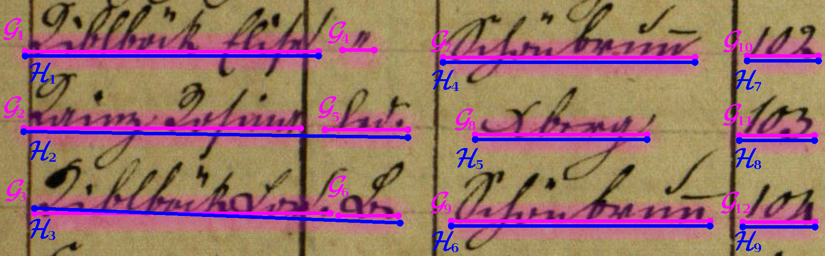
We focus on the top right four text lines of Fig. 1 to demonstrate the effect for a simple example, i.e.,

In this order the HYP and GT only differ in the sorting along columns and rows as well as in one error in the hypothesis $\mathcal{H}_{7}$. Without the reading order constraint we get $LD_{\mathcal{A}}{\left(\textbf{H},\textbf{G}\right)}=LD{\left(\mathcal{H}_{7},\mathcal{G}_{10}\right)}=1$, because $W={\left\{{\left(1,1\right)},{\left(3,2\right)},{\left(2,3\right)},{\left(4,4\right)}\right\}}$ is feasible and there are no errors in three out of the four assigned text lines. In contrast, with the constraint $A\in{\mathcal{A}^{R}}$ we get $W={\left\{{\left(1,1\right)},{\left(3,2\right)},{\left(4,4\right)}\right\}}$. The assignment ${\left(2,3\right)}$ is not allowed due to the reading order constraint. Consequently, $\mathcal{H}_{7}$ and $\mathcal{G}_{10}$ are not assigned, which results in $U={\left\{2\right\}}$, $V={\left\{3\right\}}$ and $LD_{\mathcal{A}}{\left(\textbf{H},\textbf{G}\right)}={\left|\mathcal{H}_{7}\right|}+{\left|\mathcal{G}_{10}\right|}=5$,

Based on (6) we define

as minimal LD between H and G that penalizes reading order errors and $CER^{R}{\left(\textbf{H},\textbf{G}\right)}:=\frac{LD^{R}{\left(\textbf{H},\textbf{G}\right)}}{{\left|\textbf{G}\right|}}$.

Especially for tables with short text lines containing for instance the age, the birth date or running numbers, it is possible that the minimization of (6) assigns a wrongly transcribed HYP text line to a GT text line which is located at an entirely different position in the image. E.g., $\mathcal{H}_{9}=\mathcal{G}_{10}$ holds for the text lines of Fig. 1, but their geometric positions do not match. An assignment of such kind could erroneously reduce the CER. Consequently, it makes sense to only allow assignments between $\textbf{H}_{y}$ and $\textbf{G}_{x}$ if their geometric positions match. Again, the idea is to add restrictions for $\mathcal{A}$, such that two text lines can only be assigned, if they are “(geometrically) close” to each other. There are many possibilities to determine if two text lines are close to each other or not. Here, the well-established method of [3] is used. We say two text lines are close, if their baselines are geometrically close to each other (see Section III-B for details). Let $\mathcal{N}{\left(\textbf{G}_{x}\right)}\subset\textbf{H}$ be the set of all text lines in H, that are close to $\textbf{G}_{x}$. We extend (5) to

and modify (6) with $\mathcal{A}^{G}$

to define $CER^{G}{\left(\textbf{H},\textbf{G}\right)}:=\frac{LD^{G}{\left(\textbf{H},\textbf{G}\right)}}{{\left|\textbf{G}\right|}}$.

If an LA does not detect a text line $\textbf{G}_{x}$, the LD increases by ${\left|\textbf{G}_{x}\right|}$, as well as the LD increases by ${\left|\textbf{H}_{y}\right|}$ for an erroneously detected text line $\textbf{H}_{y}$. Even more crucial are falsely merged text lines. For example, the hypothesis ${\left(\mathcal{H}_{2}\right)}$ of Figure 1 is an erroneously merged text line. For

the calculation $LD{\left(\textbf{H},\textbf{G}\right)}$ leads to $U=\emptyset,V={\left\{2\right\}},W={\left\{{\left(1,1\right)}\right\}}$ and $LD{\left(\textbf{H},\textbf{G}\right)}=LD{\left(\mathcal{H}_{2},\mathcal{G}_{2}\right)}+{\left|\mathcal{G}_{5}\right|}=5+4=9$. The resulting LD could be considered to be quite high based on the fact, that the recognized text is entirely correct, but merged. The same argument is valid for an erroneous split of a text line. Hence, it is meaningful to modify the LD calculation such that it does not penalizes this kind of split and merge errors.

It is assumed that these kind of segmentation errors are mainly caused by large gaps between words. As a result, the most common substitution for a line break is the space character $\text{\textvisiblespace}\in\Sigma$ in the merged line. Hence, we allow to interpret a line break as space character and the other way around. This is achieved by allowing successive split operations at spaces and merge operations between lines to adjust H:

• •

  split operation: One line $\textbf{h}=\textbf{H}_{y}$ with the space character $\textbf{h}_{k}=\text{\textvisiblespace}$ at position $k$ can be split into two lines $\textbf{a}={\left(\textbf{h}_{1},\ldots,\textbf{h}_{k-1}\right)}$ and $\textbf{b}={\left(\textbf{h}_{k+1},\ldots,\textbf{h}_{{\left|\textbf{h}\right|}}\right)}$,

• •

  merge operation: Two subsequent lines $\textbf{a}=\textbf{H}_{y}$ and $\textbf{b}=\textbf{H}_{y+1}$ can be merged into one line ${\left(\textbf{a}_{1},\ldots,\textbf{a}_{{\left|\textbf{a}\right|}},\text{\textvisiblespace},\textbf{b}_{1},\ldots,\textbf{b}_{{\left|\textbf{b}\right|}}\right)}$.

We define the space of partition functions

with $\Phi$ as a composition of split and merge operations. We change (6) by optimizing over all $\Phi$ that minimizes the LD:

and get $CER^{S}{\left(\textbf{H},\textbf{G}\right)}:=\frac{LD^{S}{\left(\textbf{H},\textbf{G}\right)}}{{\left|\textbf{G}\right|}}$. For the example in (10) and the optimal $\Phi^{*}$ we get

which leads to $CER^{S}{\left(\textbf{H},\textbf{G}\right)}=CER{\left(\textbf{H}^{\prime},\textbf{G}\right)}=0$.

It has to be mentioned, that ${\left|\textbf{H}\right|}\neq{\left|\Phi{\left(\textbf{H}\right)}\right|}$ is possible. Furthermore, for an optimal $\Phi^{*}$ there is no text line $\textbf{H}_{y}\in\Phi^{*}{\left(\textbf{H}\right)}$ in $U$ which contains spaces, because a splitting of $\textbf{H}_{y}$ at this spaces would result in a lower LD.

The equations (7), (9) and (12) are defined as single modifications of (6), whereby in many scenarios a combination of these modifications is reasonable: For example to measure the quality of a text extraction method, the semantic meaning is important, which leads to the reading order restriction combined with the option to change the segmentation. We will denote combinations of configurations by adding all modification letters to the superscript (in the previous example: $CER^{R,S}$). Having $3$ modifications we can choose between $2^{3}=8$ configuration-dependent CER measures.

Besides the possibility to evaluate the quality of an HTR engine under different restrictions, a meaningful comparison of the results for different measure configurations allows for an examination of the categories of the main errors of this system.

The WER can be determined based on the CER methodology introduced in this chapter. If $\Sigma$ is not chosen as alphabet of characters but of words instead, everything in Section II holds and the $CER$ becomes the $WER$. Hence, the $WER$ with all different configurations can be calculated.

There is no general definition of how to transform a sequence of character into a sequence of words. For example, the sequence ‘‘it’s’’ could be divided into one, two or three words. Since in the most cases the user has his own idea of ‘‘words’’, we provide a simple interface to integrate own word tokenizers²² 2 Interface: https://github.com/Transkribus/TranskribusInterfaces/blob/ master/src/main/java/eu/transkribus/interfaces/ITokenizer.java. A basic tokenizer, that splits a character sequence at spaces, is implemented as default. For Figure 2 this tokenizer is used.

At first glance $CER$ does not have much in common with $BOW$. However, by successively changing the configurations, we can close the gap between these measures:

So far, it is not obvious, why $WER^{S}\leftrightarrow BOW$ is reasonable. For the $WER$ calculation we do not only count the manipulations insertion, deletion and substitution, we also count the number of correctly assigned characters/words ($COR$). For the $BOW$ measure the false positive ($FP$), the false negative ($FN$) and the true positive ($TP$) words are counted. So we can define precision and recall for $WER$ and $CER$ with similar counts used in $BOW$:

whereas ${\left|GT\right|}$ and ${\left|HPY\right|}$ are the number of characters/words in GT and HYP. Note that in Figure 2 for precision and recall for $WER^{S}$ and $BOW$ are equal, even with additional geometric restrictions. Since $WER^{S}$ is constructed to minimize the LD, which only implicitly maximizes $COR$, the inequality is obvious. But if the lines of G or H are single words, it follows equality and we closed the gap between $WER^{S}$ and $BOW$.

We use the recursion defined in (II) and expand it to calculate the LD across text lines for the flattened $\textbf{h},\textbf{g}$. For that purpose, we expand (1) to

This adaptation will prevent substitutions of usual characters by line break characters and vice versa. Consequently, only line breaks can be mapped to each other. Hence, this enforces a direct comparison of entire text lines instead of parts of text lines. Let $\textbf{b}_{\textbf{h}}\in{\left[{\left|\textbf{h}\right|}\right]}^{{\left|\textbf{H}\right|}+1}$ be the tuple of line break positions in h, whereas $\textbf{b}_{\textbf{h}}^{y}:={\left(\textbf{b}_{\textbf{h}}\right)}_{y}\in{\left[{\left|\textbf{h}\right|}\right]}$ is the index of the $y$-th line break in h. The tuple $\textbf{b}_{\textbf{g}}$ is defined in the same manner. For simplification we use the notation of the cross product of sets for tuples:

For index pairs ${\left(i,j\right)}\in\textbf{b}_{\textbf{h}}\times\textbf{b}_{\textbf{g}}$ which represent line breaks at $i=\textbf{b}_{\textbf{h}}^{y}$ and $j=\textbf{b}_{\textbf{g}}^{x}$, we modify the distance calculation in (II) to allow for the deletion and insertion of lines

for other index pairs ${\left(i,j\right)}\in{\left({\left[{\left|\textbf{h}\right|}\right]}\times{\left[{\left|\textbf{g}\right|}\right]}\right)}\setminus{\left(\textbf{b}_{\textbf{h}}\times\textbf{b}_{\textbf{g}}\right)}$ we set

In the following, we use the term points for index pairs.

The calculation of $\Delta_{{\left|\textbf{h}\right|},{\left|\textbf{g}\right|}}^{R}$ can be formulated as shortest path problem. Therefore, we search the shortest path from point ${\left(0,0\right)}$ to ${\left(i,j\right)}$, which indicates the minimal cost to map $\textbf{h}_{1:i}$ to $\textbf{g}_{1:j}$. For ${\left(i,j\right)}={\left({\left|\textbf{h}\right|},{\left|\textbf{g}\right|}\right)}$ we obtain $LD^{R}{\left(\textbf{H},\textbf{G}\right)}=\Delta_{{\left|\textbf{h}\right|},{\left|\textbf{g}\right|}}^{R}$. Since at each point we calculate the minimum over other points with additional non-negative costs, we can use the Dijkstra Algorithm to solve this problem [7]. Especially for a low CER this algorithm can skip the calculation of many points ${\left(i,j\right)}\in{\left[{\left|\textbf{h}\right|}\right]}\times{\left[{\left|\textbf{g}\right|}\right]}$. The implementation is done in Java and freely available on GitHub³³ 3 https://github.com/CITlabRostock/CITlabErrorRate under the Apache License.

As mentioned in Section II-B it is reasonable to allow ${\left(y,x\right)}\in W$, only if $\textbf{H}_{y}$, $\textbf{G}_{x}$ are geometrically close to each other ($\textbf{H}_{y}\in\mathcal{N}{\left(\textbf{G}_{x}\right)}$). To define the neighborhood of $\textbf{G}_{x}$ we use a method that compares the so-called baselines of the text lines. This is a common measure to evaluate the performance of a layout analysis result [3]. We call the tuple of two-dimensional points $B={\left(B_{1},\ldots,B_{{\left|B\right|}}\right)}\in\mathbb{P}:={\left(\mathbb{N}^{2}\right)}^{*}$a baseline. We define

as tuple of polygons corresponding to H and let $\textbf{B}^{\textbf{G}}$ be defined in the same manner for G. From [3, Section III A. 3)] we use the Coverage Function $COV:\mathbb{P}\times\mathbb{P}\times\mathbb{R}\to{\left[0,1\right]}\subset\mathbb{R}$, which calculates the overlapping between two baselines for a given tolerance value. The tolerance value $t:\mathbb{P}^{*}\times\mathbb{N}\to\mathbb{R}$ is dependent on the geometric position of all ground truth baselines and the index of the ground truth baseline of interest (cf. [3, Section III A. 2)]).

We set

which implicitly restricts the set of valid assignment matrices in (5). Indeed, setting baselines to be close if they have any connection is probably a very soft restriction, but reasonable to avoid erroneously non-assignments for close $\textbf{H}_{y}$ and $\textbf{G}_{x}$. We modify (III-A) with $i=\textbf{b}_{\textbf{h}}^{y}$ and $j=\textbf{b}_{\textbf{g}}^{x}$ by

If we allow $\Phi\in\Psi$ to be applied to H, we have to modify the LD calculation at some positions. As argued in Section II we allow to map $\dlsh$ to ␣ without costs and vice versa. We define $\overline{\textbf{b}}_{\textbf{h}}$ as expansion of $\textbf{b}_{\textbf{h}}$ by also containing the positions of the space character $\text{\textvisiblespace}\in\Sigma$. We modify (16) by

and (III-A) in points ${\left(i,j\right)}$ with $i=\overline{\textbf{b}}_{\textbf{h}}^{y}$ and $j=\textbf{b}_{\textbf{g}}^{x}$ by

which also allows to skip single words. This leads to the updated Algorithm 2, which implicitly returns the best segmentation $\textbf{H}^{\prime}:=\Phi{\left(\textbf{H}\right)}$.

References

• [1] J. Sivic and A. Zisserman, “Efficient visual search of videos cast as text retrieval,” IEEE Transactions on Pattern Analysis and Machine Intelligence, vol. 31, no. 4, pp. 591–606, 4 2009.
• [2] U.-V. Marti and H. Bunke, “Using a statistical language model to improve the performance of an HMM-based cursive handwriting recognition system,” in Hidden Markov models: applications in computer vision. World Scientific, 2001, pp. 65–90.
• [3] T. Grüning, R. Labahn, M. Diem, F. Kleber, and S. Fiel, “READ-BAD: A new dataset and evaluation scheme for baseline detection in archival documents,” CoRR, vol. abs/1705.03311, 2017. [Online]. Available: http://arxiv.org/abs/1705.03311
• [4] M. Murdock, S. Reid, B. Hamilton, and J. Reese, “ICDAR 2015 competition on text line detection in historical documents,” in Proceedings of the International Conference on Document Analysis and Recognition, ICDAR, vol. 2015-November. IEEE, 8 2015, pp. 1171–1175.
• [5] S. Pletschacher and A. Antonacopoulos, “The page (page analysis and ground-truth elements) format framework,” in 2010 20th International Conference on Pattern Recognition, 8 2010, pp. 257–260.
• [6] V. I. Levenshtein, “Binary codes capable of correcting deletions, insertions, and reversals,” in Soviet physics doklady, vol. 10, no. 8, 1966, pp. 707–710.
• [7] E. W. Dijkstra, “A note on two problems in connexion with graphs,” Numer. Math., vol. 1, no. 1, pp. 269–271, Dec. 1959. [Online]. Available: http://dx.doi.org/10.1007/BF01386390