JLAB-THY-19-3022
Covariant Spectator Theory of scattering: Deuteron form factors
Abstract
The deuteron form factors are calculated using two model wave functions obtained from the 2007 CST high precision fits to scattering data. Included in the calculation are a new class of isoscalar interaction currents which are automatically generated by the nuclear force model used in these fits. If the nuclear model WJC2 is used, a precision fit (/datum ) to the Sick Global Analysis (GA) of all elastic scattering data can be obtained by adjusting the unknown off-shell nucleon form factors (discussed before) and (introduced in this paper), and predicting the high behavior of the neutron charge form factor well beyond the region where it has been measured directly. Relativistic corrections, isoscalar interaction currents, and off-shell effects are defined, discussed, and their size displayed. A rationale for extending elastic scattering measurements to higher is presented.
I Introduction
I.1 Background
This work is the last in a series of papers Gross:2014zra; Gross:2014wqa; Gross:2014tya (referred to as Refs. I, II, and III) that present the fourth generation calculation of the deuteron form factors using what is sometimes called the Covariant Spectator Theory (CST) Gross:1969rv; Gross:1972ye; Gross:1982nz. The third generation, done by Van Orden and collaborators in 1995 VanOrden:1995eg, calculated the form factors from a variation of model IIB (originally obtained from a 1991 fit to the database Gross:1991pm, with an improved fit giving /datum VanOrden:1995eg) already provided an excellent description of the deuteron form factors. The current calculation is needed only because a better CST fit to the database was found in 2007. This fit, with a /datum , included momentum dependent terms in the kernel and requires a completely new treatment. For a brief review of the previous CST history of calculations of the form factors, see the introduction to Ref. I. For a more comprehensive survey of the field see several recent reviews Garcon:2001sz; Gilman:2001yh; Marcucci:2015rca.
The CST, in common with other treatments based on the assumption that scattering can be explained by the ladders and crossed ladders arising from the exchange of mesons between nucleons Gross:1982nz; Pena:1996tf, treats nucleons and mesons as the elementary degrees of freedom, with the internal structure of the nucleons and mesons treated phenomenologically. This means that, in particular, the electromagnetic form factors of the nucleons that are bound into a deuteron are not calculated, but must be obtained from direct measurements of electron-nucleon scattering. If the form factors cannot be measured directly, they can be treated as undetermined functions that can be fixed by fitting the theory to electron-deuteron () scattering data.
In common with the 1991 fit that lead to model IIB, the new fit to the 2007 data base Gross:2008ps; Gross:2010qm was obtained using the CST two body equation (sometimes called the Gross equation) with a one boson exchange (OBE) kernel. However, we found that a high precision fit (with /datum ) could be obtained only if the vertices associated with the exchange of a scalar-isoscalar meson, denoted , included momentum dependent terms in the form
| (1) |
where is a parameter fixed by fitting the scattering data, and are the four-momenta of the outgoing and incoming nucleons, respectively, and the are projection operators
| (2) |
which are non-zero for off-shell particles, and hence are a feature of both the Bethe-Salpeter and CST equations.
Two high precision models were found with somewhat different properties. Model WJC1 (originaly designated WJC-1), designed to give the best fit possible, has 27 parameters, , and a large . Model WJC2 (originaly designated WJC-2), designed to give a excellent fit with as few parameters as possible, has only 15 parameters, , and a smaller . Both models also predict the correct triton binding energy (see Figs. 12 and 13 of Ref. Gross:2008ps and Ref. Stadler:1996ut). The deuteron wave functions predicted by both of these models Gross:2010qm have small P-state components of relativistic origin, and the normalization of the wave functions includes a term coming from the energy dependence of the kernel, which contributes for WJC1 and for WJC2.
This momentum dependence of the kernel implies the existence of a new class of isoscalar interaction currents that will contribute to the electromagnetic interaction of the deuteron, leading to the need for this fouth generation calculation. These currents were fixed in Ref. I, and used to predict the deuteron magnetic moment (Ref. II) and the quadrupole moment (Ref. III). This paper completes this series of papers by calculating the dependence of the form factors on the momentum transfer of the scattered electron, .
In the process of fitting the data, we are able to determine two off-shell nucleon form factors and predict the high momentum behavior of the neutron electric form factor, , beyond the region where it has been measured. These and other major conclusions of this paper are discussed in detail in Sec. VI below.
I.2 Organization of the paper
This paper is organized into six sections, with most of the theoretical details moved to the Appendices. The rest of this section describes the ingredients of the calculation as simply as possible, with emphasis on the important off-shell nucleon current. A more complete discussion can be found in the Appendices and in Refs. I–III. The major results are described in Sec. II, which gives predictions that are extracted from the measurements. Sec. III shows how the individual deuteron form factors are built up from the different theoretical contributions, and Sec. IV discusses the size and importance of relativistic effects. The results for the deuteron static moments are reviewed in Sec. V, and finally I draw major conclusions in Sec. VI. The reader eager to get to the conclusions may jump to Sec. VI, and backtrack as needed to fill in the many missing details.
Seven appendices summarize many details needed for a precise understanding of this paper. Appendix A reviews the theoretical definitions of the deuteron form factors, deuteron current and deuteron wave and vertex functions, and examines how the arguments of the amplitudes are shifted by the relativistic boosts that enter into the calculation of the form factors. Appendix B derives the form of the nonrelativistic deuteron charge form factor, , in momentum space. Appendices C and D discuss some details of the extraction of the nucleon form factors from the theory, and Appendices E and F describe some theoretical transformations that facilitate the calculations. Finally, Appendix G discusses some errors that were found in Ref. II.
I.3 Diagrammatic form of the deuteron current
In CST when a OBE kernel is used to describe the interaction, the two-body current is given initially by the four diagrams shown in Fig. 1. Here, by convention, it is assumed that particle 1 is on-shell (I could have chosen particle 2 to be on-shell with corresponding changes in the diagrams), and the necessary (anti)symmetry between the two particles is contained in the kernel, which is explicitly (anti)symmetrized. In these diagrams the deuteron structure is represented by a vertex function, , in which particle 1 is on shell and particle 2 off-shell, and a vertex function in which both particles are off-shell. The vertex function is calculated directly from the deuteron bound state equation and can be calculated from .
I showed in Ref. I how the current operator shown in Fig. 1(C) can be re-expressed using an effective vertex function and a subtracted vertex function . When this is done, diagram 2(A(2)) and parts of 2(B) include the interaction current contributions originally included in diagram 1(C). The new diagram 2(B) not only includes part of the interaction current, but is also a generic way of combining the two diagrams 1(B±). The three diagrams of Fig. 2 are completely equivalent to the five diagrams shown in Fig. 2 of Ref. I and Fig. 1 of Ref. II (but the labeling of the momenta in the B± diagrams differs from the choice here).
Diagrams 2(A) and 2(A(2)) describe the interaction of the photon with particle 2, allowing particle 1 to be on-shell in both the initial and final state. The internal momenta are
| (3) |
where () are the four-momenta of the outgoing (incoming) deuterons, and the hat symbol over a four-vector means that the four-vector is on-shell. Diagram 2(B) describes all the interactions of the photon with particle 1, so that both particles must off-shell in either the initial or in the final state. Here the internal momenta are
| (4) |
The final (initial) nucleon is on shell when (), with
| (5) |
I.4 Strong form factor and the bound nucleon current
In this section I describe two central features of the CST calculation of the deuteron observables and form factors from the diagrams in Fig. 2. These are (i) the presence of a strong nucleon form factor, , and (ii) the structure of the bound nucleon current, which depends on four form factors: not only the usual Dirac and Pauli form factors and , but also two off-shell form factors and . The first of these, , has been discussed extensively in previous work, but has never been introduced before and is a major new feature of this paper.
I.4.1 The strong nucleon form factor
In all strong, nonperturbative theories of hadronic structure there is a need to include form factors that cut off high momentum contributions and provide convergent results. In the CST-OBE models studied so far, the form factors at the meson- vertices are assumed to be products of strong form factors for each particle entering or leaving the vertex. This means that for each nucleon of momentum entering or leaving a vertex, there is a universal strong nucleon form factor (a function of only) present at that vertex. This form factor is normalized so that when (so that is on shell), .
Because it is universal, the strong form factor associated with each external nucleon line can be factored out from the scattering kernel giving
| (6) |
where () are the four-momentum of the outgoing (incoming) particle 1, is the reduced kernel and, for both primed and unprimed variables, . Note that the expression for the kernel is written allowing for the possibility that any (or all four) of the particles could be off-shell. Similarly, removing the strong form factors from the vertex function gives a reduced vertex function , where
| (7) |
Since is included in the kernel, and when particle 1 is on-shell, the dependence of the results on variations of when particle 1 is on-shell has already been studied in the fits to the scattering and presents nothing new. However, when electromagnetic current conservation is imposed, the presence of leads to a modification of the nucleon current. This dependence is a new feature of the relativistic theory that is interesting to study. In addition, when particle 1 is off-shell, so that , the dependence of the calculation on for is another feature of the relativistic theory that is new.
I will report on some of these effects later in Sec. III; for now I only want to highlight existence of the strong form factor , because its presence drives the discussion of the bound nucleon current.
I.4.2 Structure of the bound nucleon current
Using interactions that depend only on , the momentum transfer by the interacting particles, Feynman showed a long time ago that current conservation could be proved if the off-shell bound nucleon current satisfied the Ward-Takahashi (WT) identity
| (8) |
where is the propagator of a bare nucleon, which in my notation (with the ’s removed) is
| (9) |
When a strong nucleon form factor is present, the interactions in a one boson exchange (OBE) model will be of the form , and can be made to depend only on if the strong nucleon form factors coming from the initial and final interactions that connect each propagator are moved from the interactions to the propagators connecting them. Since each propagator connects two interactions, the new (dressed) nucleon propagator then has the form
| (10) |
Now a similar proof of current conservation is possible Gross:1987bu provided a reduced current , is constructed
| (11) |
and required to satisfy a generalized WT identity
| (12) |
There are many solutions to (12). The one I use in this paper is
| (13) | |||||
where are (uniquely determined) off-shell functions discussed below, is the isoscalar charge, the off-shell projection operator was defined in (2),
| (14) | |||||
and the transverse gamma matrix is
| (15) |
with . Except for the addition of the new form factor , this is precisely the current that has been used in all previous work.
I.4.3 Uniqueness of the bound nucleon current, and the principle of balance
The longitudinal parts of the current (13) are largely determined by the generalized WT identity (12). Still, as (14) displays, the important physics contained in the form factors and is purely transverse, and the longitudinal part that is constrained by the WT identities will not contribute to any observable since it is proportional to which vanishes when contracted into any conserved current or any of the three polarization vectors of an off-shell photon. The form factors themselves are completely unconstrained by current conservation, except for the requirement that (with the real normalization set by ). This is as it should be; the structure of the nucleon should not be fixed by the general requirement of current conservation.
Similarly, the transverse Pauli-like terms and are completely unconstrained, and there are may other off-shell terms that we could add to the current. What principal is to constrain these?
In Ref. I, I introduced the principles of simplicity and picture independence in an attempt to limit possible contributions. I found that, using current conservation and these principles, all contributions from the structure of the meson-nucleon vertices could be expressed in terms of the nucleon structure alone; no new interactions, such as the famous interaction current, needed to be added. However, these arguments placed no constraint on the term. Clearly it must be included because the free nucleon cannot be described without it, but the choice of whether or not to multiply the term by is not dictated by these principles. Similarly, I emphasize that the introduction of is not required by the principles of simplicity or picture independence. To justify the introduction of and to explain the use of the same for both and , and the same terms for and , a new principle is needed.
The new principle will be referred to as the principle of balance between Dirac and Pauli interactions. The principle states that whenever a Dirac-like charge term ( and in this case) is required, a similar Pauli-like term ( and ) will be included. This ensures that the off shell current, expressed in terms of the and from factors, could also be expressed in terms of off-shell charge () and magnetic () form factors, without a constraint on the structure of either (except for the previously discussed constraint ).
I.4.4 Properties of and
The simplest solution to (12) is
| (16) |
where I use the the shorthand notation and . Both and are symmetric in , and important limits are
| (17) |
where
| (18) |
I.5 Definitions of deuteron observables
Precise definitions of the deuteron form factors will be reviewed in Appendix A. For an understanding of the results to be presented in Sec. II, it is only important to review that electron-deuteron scattering is described by three independent deuteron form factors Garcon:2001sz; Gilman:2001yh: (charge), (magnetic), and (quadrupole). Denoted generically by (with ). These form factors are a sum of products of isoscalar nucleon form factors, (where the subscript labeling these as isoscalar will be omitted throughout this paper for simplicity), and body form factors, , so that
| (19) |
It is important to realize that the theory presented in this paper calculates the body form factors only; the nucleon form factors must be obtained from another source.
The deuteron form factors can be measured by the analysis of three independent experiments. Two of these can be obtained from the unpolarized elastic scattering of electrons from the deuteron. In one photon exchange approximation, this elastic scattering is given by
| (20) |
where
| (21) |
is the cross section for scattering from a particle without internal structure ( is the Mott cross section), and , , and are the electron scattering angle, the incident and final electron energies, and the solid angle of the scattered electron, all in the lab system. The structure functions and , which can be separated by comparing unpolarized measurements in the forward and backward directions, depend on the three electromagnetic form factors
| (22) |
where
| (23) |
To further separate and , the polarization of the outgoing deuteron can be measured in a separate, analyzing scattering. The quantity most extensively measured is
| (24) |
where
| (25) |
Note that the structure function depends only on , and depends on , both of which are linear in the the nucleon form factors. However, the structure function is quadratic in the nucleon form factors.
II Fits to the Deuteron Observables
II.1 Introduction
All results for the deuteron form factors depend on the off-shell nucleon form factors and . However, except for the sole requirement that , these form factors are completely unknown, and it is appropriate to use the deuteron form factor data to determine them. The first step, determining and , in done in Sec. IIB below.
I have found that the most efficient way to do this is to use the data from (determined directly from ) and [actually from Eq. (25)]. Both and are linear in and , so a solution is straightforward and it is easy to determine the errors in and from the errors in and . Details are given in Appendix C.
The data are scattered, and to do this efficiently it would first be necessary find a smooth fit to all the data. Fortunately, Sick has produced a Global Analysis Sick:2001rh; Marcucci:2015rca (referred to as the GA in this paper) where he reanalyzed all of the data starting from the detailed records. I will use his GA for a representation of the data. Once and have been determined, the data (that is, the Sick GA) for and is exactly reproduced, as shown in Sec. IIC.
Note that determines only the ratio of the independent form factors and , not their size. The third observable, , can vary even when and are fixed. This is studied in Sec. IID, where it is shown that can be adjusted to give the correct (fortunately, and are very insensitive to , so that this determination of does not alter the fits to and ). The predictions for made by each model is discussed in Sec. IID, where it is shown that model WJC1 fails at this point, but model WJC2 works very well. Finally, using the predicted and and various models of , Sec. IIE presents the deuteron form factors and compares them to Sick’s GA.
In order to keep the number of figures to a minimum, the reader is warned that some of the early figures will show results for models that will not be introduced until later in the discussion. To help with this, all of the models that will be used are summarized in Table 1. Models 1A and 2A are a starting point; their input is the same as the successful VODG calculation (except I never have any interaction current). Model VODG used the GK05 prediction of , and in the absence of any previous knowledge, assumed a standard dipole for and . Then, models 1B and 2B replace and by the solutions found in Sec. IIB, giving precise fits to and . Finally, models 2C and 2D show the results of using models for based on the predictions given in Sec. IID, and cannot be understood until that section is studied.
| Name | Deuteron | color | line | |||
| VODG* | IIB | GK05 | dipole | 0 | black | long-dash |
| VODG0 | IIB | GK05 | dipole | 0 | black | 2 dash-2 dot |
| 1A | WJC1 | GK05 | dipole | 0 | blue | short-dash |
| 2A | WJC2 | GK05 | dipole | 0 | red | short-dash |
| 1B | WJC1 | GK05 | blue | 2 dash-2 dot | ||
| 2B | WJC2 | GK05 | red | 2 dash-2 dot | ||
| 2C | WJC2 | CST2 | red | long dash-dot | ||
| 2D | WJC2 | CST1 | red | thick solid |
*Model VODG includes a exchange current calculated using the Rome 2 form factor Cardarelli:1995ap.
II.2 Predictions for the off-shell nucleon form factors
As mentioned in the Introduction, the off-shell form factors can be found by simultaneously fitting them to the GA data points for and (which is independent of ). Each GA point has its own error that I use to estimate the errors in the fitted values of the form factors. The results obtained from Models WJC1 and WJC2 are shown in Figs. 3 and 4. Each red and blue point in the figure is the (simultaneous) solution for and at each GA point, which extend out to = 7 (fm)-1 = 1.379 (GeV) (limited my the measurements of ).
On the same figures I also show the values obtained by fitting separately to (solid black diamonds) or (half filled black diamonds) under the assumption that . The fact that these fits differer substantially shows that it is not possible to obtain a good fit to the GA data without including a nonzero .
| (1) | (2) | (1) | (2) | |
|---|---|---|---|---|
| 30.905 | 1.3508 | 29.467 | 1747.8 | |
| 457.66 | 4.0568 | 1141.0 | 2395.0 | |
| 1401.7 | 0 | 2422.0 | 0 | |
| 1618.9 | 137.69 | 404.21 | 3370.4 | |
| 1.2323 | 0.6131 | 1.1115 | 1.0004 |
Note that the form factors are largely undetermined at GeV, and also at small where the errors in the fitted form factors are large. In order to have results for all , and especially beyond the range where data for exists, I chose smooth curves that fit the points in the range 0.5 GeV, where they are well constrained. The generic models used for and are
| (26) |
where for WJC1, for WJC2, and the other parameters are given in Table 2. The asymptotic limits of these form factors are
| (27) |
and note that I have constrained
| (28) |
Finally, I point out that the models for those form factors are real analytic functions with cuts in the complex plane along the positive real axis. For the model WJC2, these cuts start at
| (29) |
Both cuts start near or above the the 7 threshold, confirming that they are short range effects. Similar results hold for . I have not investigated the dispersion relations that these functions satisfy.

II.3 Fits to and
With the off-shell form factors determined, I now confirm that the fits to and do indeed agree with the Sick GA. (The fits to , related to , will be shown later when the other form factors are discussed.) This is also an opportunity to compare the results for Models WJC1 and WJC2 with the previous successful calculation of Van Orden et al.VanOrden:1995eg, which is refered to as VODG. The various models under discussion in this and the following sections are defined in Table 1, and will be referred to by the simple names given in the table.
I begin by showing the data for in Fig. 5. The rapid variation of with makes it difficult to see how the theory compares with data, so I have scaled everything by the simple fit function
| (30) | |||||
where is measured in GeV, and the tail was adjusted to be near an expected secondary maximum in . The results of dividing both data and predictions by this function are shown in Fig. 6. This figure also shows how the various theoretical models shown in Table 1 compare with the experimental data and the Sick GA. Fig. 7 shows how the models and Sick GA compare with the experimental data for .
Study of the curves in Figs. 6 and 7 show that models 1A and 2A, with the same assumptions as VODG (standard dipole for , , and GK05 nucleon form factors) are both successful at low GeV, but 1A seriously overshoots B at higher and 2A undershoots already at about . Model VODG overshoots a little near GeV (this will be more clearly displayed when we show below), but the discrepancy is smaller than either Models 1A or 2A. VODG gives a better explanation than either models 1A and 2A.
As expected models 1B and 2B, that use the appropriate and for each model, do indeed give excellent agreement with the structure function and over the entire region where the GA exists. Note that the size of the exchange current used by VODG can be inferred from the differences between VODG0 and VODG and is smaller than the effects arising from and , particularly for model WJC2.
Finally, the figures show the important result that the best models, 2C and 2D that have not yet been introduced, are practically indistinguishable from 2B in the region of the GA fit. Their significance will be discussed in the next section.
II.4 Predictions for and
To complete the picture, Fig. 8 shows the data and predictions for similar to those shown for in Fig. 5. This figure shows nicely how falls as an exponential over many decades. As was the case or , comparing theory to data on such a curve obscures all but huge differences. To see differences of a factor of 2 or 3, the structure function is scaled by the simple function
| (31) |
(where Q is measured in GeV), and Figs. 9 and 10 show these scaled results, which play a role in our discussion of similar to that played by Fig. 6 in our discussion of . To emphasize the differences at large , Fig. 10 is the same as Fig. 9, but with the scales expanded.
Figs. 9 and 10 show that all theoretical models give an excellent description of at GeV. However (excluding models 2C and 2D for now) none of the models do very well describing the GA significantly above GeV. VODG does the best (with the exchange current playing a decisive role), model 2B is not far off, but models 1A and B, and 2A all depart substantially from the GA and are clearly unacceptable. This means that even when the two unknown off-shell form factors and are adjusted to fit and , Model WJC1 disagrees with the data for by such a large amount that it cannot be repaired, as discussed in the next section.
Note that model 2B does well out to GeV, but dips below the data in the region from GeV. This is a region where the nucleon charge form factor, is unknown, and hence this calculation can be used to predict in this region.
Models 2C and 2D will be discussed below, and the failure of any of the models to describe at the highest values of will be discussed in the Conclusions.
The values of required to bring each model into agreement with the GA points for are shown in Fig. 11. The GA fits to , shown Figs. 9 and 10, extend out to (GeV) = 8 (fm)-1, well beyond the region where is known. However, since is quadratic in (but only one root is acceptable; see the discussion in Appendix D), there is no guarantee that a real solution can be found at each point. It is remarkable that real solutions do exist except at the highest values of . I found that there were no solutions for Model WJC1 at the 3 highest GA points ( GeV), and for WJC2 at the 5 highest GA points ( GeV). The errors shown are determined by the GA errors in only; at high the theory depends on the extrapolations obtained from the fits and (where ), and hence are subject to additional errors I have not tried to estimate.
Here we have a very different situation from our previous study of and . Measurements of from free neutrons using recoil polarization, Eden:1994ji–Plaster:2005cx are completely independent of any theory of the deuteron, and those from a polarized deuteron target, Passchier:1999cj–Warren:2003ma, are almost as clean. All of these measurements are shown in Fig. 11, and I chose to focus only on them because they are insensitive to deuteron theory. For a recent review of the experimental data, see Ref. Perdrisat:2006hj; many other measurements exist.
Fig. 11 shows that the solution for for Model WJC1 is in serious disagreement with the form factor measurements from free neutrons. There seems to be no way to repair model WJC1; for this reason I did not study the predictions for model WJC1 further.
In contrast, the solution for from model WJC2 is in good agreement with the free data. To study various possibilities, I decided to represent by the general functional form
| (32) |
which goes like at large , and has cuts only for positive , required if it is to be represented by a dispersion relation. This functional form is so flexible that it can describe GK05 and two additional models of potential interest. The parameters used for these three models of are given in Table 3. Model CST1 is a very good representation of the solution obtained from , while model CST2 follows GK05 up to the highest points (Mad03,Pla05) and then tracks CST1 at higher . All three of these models are shown in Fig. 11.
It turns out that both and are very insensitive to , so our choice of a new different from GK05 will not disturb our previous fits to and (this can be confirmed by noting that the left panels of Figs. 6 and 7 show almost no differences between models 2B, 2C, and 2D in the regions where they were used to obtain and ). Hence the only effect of choosing a new is an improvement in , and as Fig. 10 showns, model 2D (with represented by model CST1) provides an excellent fit to the data (except at the highest points – to be discussed in the Conclusions), while model 2C (with represented by model CST2) is almost as good, and this tracks GK05 in the region where has been measured. Final conclusions will be drawn in Sec. VI.
Predictions for the three form factors , , and are shown in the next subsection.
| GK05 | CST1 | CST2 | |
| 0.4779 | 0.4930 | 0.4930 | |
| 0.5798 | 16.254 | 0.5532 | |
| 1.8452 | 27.849 | 0.6805 | |
| 0.4045 | 33.710 | 0.6861 | |
| 0.8628 | 1.5836 | 0.7904 |
| 0.6743 | 0.5149 | 0.4980 | |
| 0.0693 | 0.2912 | 0.0559 | |
| 0.0084 | 0.0013 | 0.00008 | |
| 1.8478 | 1.8422 | 1.2732 | |
| 0.4185 | 0.5252 | 0.2956 | |
| 0.1557 | 0.1749 | 0.0963 | |
| 0.0321 | 0.0204 | 0.0194 |
II.5 Predictions for the deuteron form factors
I now can complete the discussion by presenting the three deuteron form factors and comparing them to Sick’s GA, which has been determined in the region GeV.
In order to better see the details, all form factors are normalized to unity at , and divided by scaling functions with the same functional form as used in Ref. Marcucci:2015rca:
| (33) |
where
| (34) |
ensuring that ScaleG. In order to scale the large behavior of the form factors, I found it necessary to refit the coefficients, and the values I use in this paper are given in Table 4.
| nbr of points | 2C | 2D | |
|---|---|---|---|
| 28 | 3.613 | 0.116 | |
| 32 | 0.713 | 0.763 | |
| 28 | 1.920 | 0.446 | |
| 44 | 6.440 | 0.774 | |
| tail | 5 | 125.1 | 116.5 |
| 34 | 1.130 | 1.131 | |
| 28 | 0.127 | 0.131 |
| number | /d | number | /d | ||
| HEPL-65 | 5 | 2.53 | Bates-84 | 2 | 0.13 |
| Orsay-66 | 4 | 1.63 | Nuovo-85 | 2 | 0.78 |
| CEA-69 | 18 | 3.01 | Nuovo-90 | 2 | 0.83 |
| DESY-71 | 10 | 0.71 | Bonn-91 | 1 | 0.55 |
| SLAC-75 | 8 | 1.61 | Bates-94 | 3 | 2.50 |
| Mainz-81 | 18 | 7.36 | NIK-96 | 1 | 1.02 |
| Bonn-85 | 5 | 20.18 | NIK-99 | 3 | 0.70 |
| Saclay-90 | 43 | 2.77 | JLabC-00 | 6 | 0.86 |
| JLab-A | 16 | 4.59 | Nuovo-01 | 5 | 3.14 |
| JLab-C | 6 | 2.87 | Bates-11 | 9 | 0.94 |
| All | 131 | 3.98 | All | 34 | 1.29 |
| ranges | |||||
| GeV | 64 | 3.82 | Stan-65 | 4 | 1.08 |
| GeV | 67 | 4.14 | Mainz-81 | 4 | 2.87 |
| 3 largest | 3 | 21.83 | Saclay-85 | 13 | 0.75 |
| Bonn-85 | 5 | 1.07 | |||
| JLab-89 | 6 | 2.06 | |||
| SLAC-90 | 9 | 2.28 | |||
| All | 41 | 1.56 |
| Relativistic vertex function (with particle 1 | |
| on-shell); contributes to all diagrams shown in | |
| Fig. 2; solution of a two-nucleon CST equation | |
| using the OBE kernel | |
| Relativistic wave function (with particle 1 | |
| on-shell); generated by interaction currents | |
| of type which arise from the momentum | |
| dependence of the boson couplings to particle | |
| 2; calculated by iterating the CST equation | |
| once using the kernel ; diagram 2(A(2)) | |
| Subtracted vertex function (with both particles | |
| off-shell); the subtraction arises from the | |
| interaction currents coming from the | |
| momentum dependence of the boson couplings | |
| to particle 1; calculated by iterating the CST | |
| equation once using the subtracted kernel | |
| with both particles off-shell in the | |
| final state; diagram 2(B) | |
| and | Form factors describing the off-shell nucleon |
| current; diagram 2(A) |
The scaled deuteron form factors are shown in Figs. 12 and 13. In the figures I display all of the cases studied in the previous sections, even though the models 2C and 2D are the only ones that are in quantitative agreement with the Sick GA.
Note that model VODG predicts all of the form factors within 1-2 standard deviations over the entire range. Model 2B, designed to agree precisely with and , gives an exact description of over the entire range (as expected) but fails to provide a precise explanation of and . In the region , both and are too large, so that their ratio, measured in , is correct. Only models 2C and 2D give a precise explanation of all form factors.
I call attention to the contributions of the and form factors which are easy to see on these plots. Since cannot be zero (because of the constraint ) the best way to isolate the size of these contributions is to compare models 1A and 1B, or 2A and 2B, shown respectively by the short dashed and double dash-dot lines (blue for WJC1 and red for WJC2). The figures show that that there is little difference at GeV, except that model 2A fails to describe even at quite small .
Table 5 shows how closely models 2C and 2D predict Sick’s GA (using Sick’s error bars). Except for few points in at the highest (the tail), the fits are excellent, of comparable quality except of , and , where model 2D provides a more accurate prediction than 2C.
Table 6 shows the /datum for the published data compared to model 2D. Note that the CST prediction is in reasonable agreement with the data for and , but that there are large discrepancies with the data for , even for GeV, and that the measurements at the three largest points (JLabA) are in significant disagreement with the perdiction (but the disagreement is not as large as with the Sick GA). I will discuss this further in the Conclusions
III Physical Insights
In this section I study the size of various partial contributions to the form factors. The study is limited to model 2D, which gives the best fit to the Sick GA. Before discussing the individual contributions, it is helpful to briefly identify the ingredients of the theory.
III.1 Physical quantities of the theory
The physical quantities that I will focus in in this section are summarized in Table 7. They are: (i) vertex functions and when one particle is on-shell, (ii) the subtracted vertex function for both nucleons off-shell, and (iii) the new off-shell nucleon form factors and already discussed extensively above. To make the presentation simple, I postpone all precise definitions until Appendix A.
III.2 Study of the isoscalar interaction currents
The isoscalar interaction currents (IC) produce the interaction current vertex function generated by and giving rise to diagram Fig. 2(A(2)), and the subtraction terms generated by and discussed in Ref. I. The behavior of these terms is shown in Fig. 14.
Fig. 14 shows that both IC’s make significant contributions to , even at low . For the other form factors, and , their contributions are quite small at low , but are still important for GeV (for ) and GeV (for ). These interaction currents are a significant part to the overall theoretical picture.
III.3 Off-shell effects
What are off-shell effects? This discussion must be approached carefully or serous misunderstandings may emerge. For example, in the CST one nucleon is always off-shell in intermediate states; this is the way the CST creates virtual intermediate states and, at the same time, preserves four-momentum conservation. In conventional quantum mechanics, the particles are always on-shell, but the virtual intermediate states do not conserve the total energy of the particles. It can be shown that these two approaches are largely equivalent, with the CST having the advantage that it is relativistically covariant, and the disadvantage that it must learn how to describe off-shell particles (with their accompanying antiparticle components). In the context of the discussion of scattering, for example, the role of the virtual antiparticles is an interesting off-shell effect. However, in the context of scattering, I will look only at new effects that did not already arise in scattering.
The unique off-shell effects that are studied here are the contributions that arise when both nucleons are off-shell. These are the contributions from the vertex functions , which take us outside the usual boundaries of the CST. The need to discuss the physics of two nucleons off-shell does not arise in the discussion of three-nucleon scattering Stadler:1996ut; Gross:1982ny; Stadler:1995cjp; Stadler:1997iu but does arise in the discussion of scattering and electron-triton scattering Pinto:2009dh; Pinto:2009jz. How should these effects be defined so that they give us useful insight into the physics of this theory?
Only diagram 2(B) requires particle 1 to be driven off-shell. In the Breit frame, , with . When the incoming (outgoing) particle 1 is on-shell, the outgoing (incoming) particle 1 will have four-momentum
| (35) |
where
| (36) |
This particle is off-shell with an energy . I find it convenient to describe this extra degree of freedom by the parameter , which is defined as the ratio of the off-shell energy to the on-shell energy. In this case the ratio is
| (37) |
which is always positive. The maximum of () occurs when (or ), , and solving for gives
| (38) | |||||
and the minimum is . This shows that as increases, the particle 1 (either incoming or outgoing) is forced further and further off-shell.
While this is useful for our understanding, what we really want is the result in the rest system of the deuteron, so (38) must be transformed to the rest system. This is discussed in detail in Appendix A.3. The results for both (38) and the relativistically correct result , given in Eq. (81), are shown in Fig. 15. Note that the boost effects are significant.
The invariants that describe depend on the two variables and (with when particle 1 is on shell). As shown in Fig. 15, for studies of the form factor below it is sufficient to know the off-shell dependence of the invariants that describe in the range . This behavior is shown in Fig. 16, with and related to the largest deuteron wave functions and by
| (39) |
The other wave functions are much smaller.
To obtain the off-shell behavior, the wave functions are iterated once using the fully off-shell kernel, as shown in Eq. (62b). I found that the resulting wave functions were much smother at low momentum if the small one photon exchange term was removed from the iterating kernel, and all of the results presented in this paper were calculated in this way. This is partly justified by the observation that keeping the “last” one photon exchange could be regarded as including one higher order effect in while ignoring others, and may not even be consistent. In any case, it introduces a small inconsistency: when the on-shell wave functions are iterated without the last one photon exchange, the normalization is changed slightly. To obtain the original normalization, the results for WJC1 are multiplied by 0.9962 and those for WJC2 by 0.9954.
The point on the curves where particle 2 is on-shell is given by
| (40) |
which depends on . This point is marked by the small solid black squares (for MeV), red diamonds ( MeV), and blue circles ( MeV) along the axis in the panels of Fig. 16. These points are interesting because the two-body bound state equation depends on vertex functions defined only at and ; values of the vertex functions at all other values of have not played any role in previous fits to the data.. The off-shell dependence of elastic ed scattering depends on values of the vertex functions determined theoretically, but never tested experimentally.
The size of these effects is shown in Fig. 17. In each panel the black dotted line is a calculation using the parameters of model 2D with in the (B) diagrams, and the thick red solid line is the full model 2D with free to vary as the kinematics dictates (as shown previously). The contribution from Fig. 2(B) decomposes into a contribution multiplied by the projector that vanishes when particle 1 is on-shell (referred to as the C contribution) and a remainder (referred to as the B contribution, distinguished from the total by the absence of the parentheses):
| (41) |
The C contribution (labeled by the blue long dashed lines in the figure) is quite small, but still of great interest because it depends on invariants that do not exist when one of the particles is on-shell. The largest off-shell contributions come from the B terms (dash-dotted blue lines), which make a significant contribution to all the form factors, especially and .
The calculations are sensitive to off-shell effects at all values of .
III.4 Size of the and contributions
The size of the and contributions was addressed in Fig. 13; Fig. 18 shows these effects in more detail. Both and make comparable contributions. It is interesting to note that the contribution plays a very important role in correcting the failure of model 2A at low . In this case the and contributions are individually quite large and tend to cancel each other.
III.5 Accuracy of the RIA
In the absence of isoscalar interaction currents, the relativistic impulse approximation (RIA) was originally defined to be twice the contribution from diagram 2(A). The interest in this approximation arose from the idea that symmetry (the CST equations are explicitly symmetrized to ensure that scattering satisfies the generalized Pauli principle exactly) should allow one to get the full result from the electromagnetic scattering from only one of the nucleons (multiplied by a factor of 2). If this were true, after adding interaction currents the results from diagrams 2(A)+ 2(A(2)) should equal the results from 2(B), so that the full result would come from either of these alone, or their average, which emerges if we take 1/2 the sum of the contributions from the lower and upper half plane.
The contributions from diagrams 2(A)+ 2(A(2)) and 2(B) are compared in Fig. 19. The contributions from 2(B) is given in two parts: the B and C contributions discussed in Eq. (41). The B contributions (labeled with the blue dot-dashed line) and the explicitly off-shell C contribution. The sum of these contributions, the total from diagram (B), is the long dashed blue line. The average of the two long dashed lines (black and blue) is the total result for model 2D.
I conclude from this figure that the RIA disagrees the the magnetic form factor even at low , but that it works reasonably well at low momentum transfer for the two charge form factors. In any case, it is not good enough to be a replacement for the full theory, as was hoped at one time.
IV Relativistic effects
Some in the electron scattering community still believe that relativistic effects are small in electron deuteron scattering and that it is possible to use deuteron wave functions calculated from the Schrödinger equation to study elastic scattering. Casper and I argued over 50 years ago Casper:1967zz that relativistic corrections were important when using deuteron scattering data to draw precise conclusions, and in this section I will review this issue in detail.
I focus only on the observables and at small , where it might be assumed that a nonrelativistic calculation would be reliable. The nonrelativistic theory for gives
| (42) | |||||
where , and are the and state wave functions, and
| (43) |
[Beware that the defined above differs significanty from the defined in Eq. (35).] This momentum space nonrelativistic result emerges naturally from the nonrelativistic limit of the CIT. This is a very general feature of this theory, and provides an excellent starting point for the study of relativistic effects. To get the right limits, one must be very careful to use the correct nonrelativistic transformations: argument shift (63c) for the (A) diagram and (71) for the (B) diagram. Both the (A) and (B) diagrams give exactly the same nonrelativistic limit, a limit where the RIA is accurate.
The size of various contributions, scaled by the nonrelativistic expression (42), is shown in the left panel of Fig. 20. The blue dashed line replaces the nonrelativistic argument shifts that appear in (42), and were derived in (63c), with the fully relativistic ones (63b). Note that this effect alone accounts for about a 4% correction at GeV, about eight times the size of the error in the Sick GA. The blue solid line shows the result obtained from the full calculation of if only and wave functions are included. At this produces a discrepancy of almost 10% with the nonrelativistic calculation. All changes after this begin to go beyond relativistic kinematics. Adding the and terms moves the result to the red dot dashed line, and adding the C contributions from the (B) diagram moves the total to the red short dashed line, both small effects. A bigger change occurs when we add in the A(2) diagram and all contributions from the nucleon form factor, bring the result to red longer dashed line. Finally adding the contributions from the off-shell form factors and brings us to the final result for model 2D, the heavy solid red line. The green short dashed line is the function
| (44) |
which gives a rough estimate of the size of all of the effects.
The size of the relativistic argument shift alone is about 4 times smaller than the total shift, or about , comparable to the result that Casper and I found over 50 years ago. For comparison, the recoil effect of the deuteron itself is very much smaller
| (45) |
Because the kinematics and the relativistic shifts in the arguments of the wave functions (that add up to the solid blue line in Fig. 20) can explain only about 1/2 of the total shift, it is clear that an accurate theoretical interpretation of the data requires the use of a relativistic theory, even at the smallest values of .
The right panel of Fig. 20 shows theory and data for the structure function , all scaled by . The red dot-dashed line is of model 2D while the thick solid line is the full calculation of using all form factors from model 2D. The panel shows that the other contributions to coming from and begin to become important at GeV.
| A | Total from diagram (A) with |
|---|---|
| full given in Eq. (16) | |
| A0 | Diagram (A) with |
| AA0 | Total dependence from diagram (A) |
| A2 | Diagram (A(2)), calculated using |
| Eq. (62a) with the interaction | |
| B, C | The two parts of diagram (B) [the B and C terms in |
| the decomposition (41)] with calculated | |
| using Eq. (62b) | |
| B0, C0 | The two parts of diagram (B) with fixed |
| at in , but not in | |
| Bh, Ch | The dependence of on in the |
| two parts of diagram (B) | |
| BBh, | Removes the dependence of on from |
| CCh | B0 and C0, leaving everywhere (on-shell) |
| on-shell | A0 + B Bh + C Ch; terms, Refs. II |
| 0.286 (1+), Ref. III | |
| AA0+ Bh + Ch; terms, Ref. II; | |
| , Ref. III | |
| A2; terms, Ref. II; 0.286 , Ref. III | |
| off-shell | BB0 + C C0; terms, Ref. II; |
| 0.286 , Ref. III | |
| (includes the current) | |
| TOTAL | A+A(2)+B+C |
V The static moments
The form factors at give the charge, magnetic, and quadrupole moments in units reported in Eq. (A.1). Using the exact equations, there is no need to expand the analytic results around as we did in Refs. II and III. However, comparison of the two different calculations uncovered some errors in Ref. II, and I now find that the new value for the magnetic moment predicted by model WJC2 is in precise agreement with the measured result. In addition the new, more accurate values of the quadrupole moment differ from the experimental values by over 1%, with no significant difference between the predictions of the two models, in disagreement with the conclusions of Ref. III.
Various contributions to the static moments are defined in Table 8. Here, in order to provide details that may be of use to future investigators, I also report some contributions that I did not study in the previous references. Tables 9 – 11 compare the results obtained from the exact form factors with the results obtained from the approximate expansions reported in Refs. II and III (and for the magnetic moment, in Appendix G).
V.1 Charge and magnetic moment
In Ref. II I conjectured that the errors in the expansions should be about 0.002. As shown in Table 9, the calculations of the charge agree to better than this, but the magnetic moment presents a more complicated picture. I originally found such large disagreements with the expansions for the magnetic moment reported in Ref. II that I redid them and found the corrected results given in Appendix G. Table 10 shows that the new expansion disagrees with the exact results by about 0.002 for several terms but there are discrepancies as large as 0.007 (0.7%) with others. I believe that the major source of this discrepancy is the expansion of the nucleon kinetic energy
| (46) |
Since terms were dropped, the discrepancy could be as large as 0.007 if the terms conspire to make the coefficient of the term of the order of unity (and not 1/8) and the mean momentum of the nucleon is about 300 MeV. In any case, the expansions are not as reliable as I expected. The remarkable new result is that the magnetic moment for model WJC2 is in very good agreement with experiment, differing by only 0.07%.
V.2 Quadrupole moment
The comparison of the quadrupole moment with the expansions reported in Ref. III does not fare much better. Here I originally estimated the error to be about or a of 0.0006, and a comparison with Table 11 shows that this seems to be accurate for the small terms, but fails for the largest terms with an error of about 0.002, or about 1% (similar to that found for the magnetic moment). However. since all terms seem to have similar signs and magnitudes, there is no reason to expect an error as I did for the magnetic moment, and I did not recalculate the expansions given in Ref. III. The new conclusion here is that the two models have similar quadrupole moments, differing by about 1.5% from the experimental result.
| Quantity | WJC1 | WJC2 | ||
|---|---|---|---|---|
| 1B | Ref. II | 2D | Ref. II | |
| on-shell () | 1.0547 | 1.055 | 1.0231 | 1.023 |
| dependence | 0.0245 | 0.025 | 0.0176 | 0.018 |
| current | 0.0228 | 0.023 | 0.0111 | 0.011 |
| off-shell () | 0.0562 | 0.057 | 0.0297 | 0.030 |
| TOTAL | 1.0002 | 1.000 | 1.0000 | 1.000 |
| 2 A0 | 1.0547 | 1.055 | 1.0231 | 1.023 |
| 2 (AA0) | 0.0245 | 0.025 | 0.0176 | 0.018 |
| 2 B | 0.9693 | — | 0.9835 | — |
| 2 C | 0.0025 | — | 0.0021 | — |
| 2 B0 | 1.0816 | — | 1.0428 | — |
| 2 C0 | 0.0025 | — | 0.0021 | — |
| 2 Bh | 0.0245 | 0.025 | 0.0176 | 0.018 |
| Quantity | WJC1 | WJC2 | ||
|---|---|---|---|---|
| 1B | App G | 2D | App G | |
| on-shell () | 0.8985 | 0.8812 | 0.8643 | 0.8630 |
| dependence | 0.0123 | 0.0145 | 0.0112 | 0.0092 |
| current | 0.0156 | 0.0167 | 0.0004 | 0.0000 |
| off-shell () | 0.0289 | 0.0170 | 0.0180 | 0.0129 |
| TOTAL | 0.8663 | 0.8620 | 0.8580 | 0.8594 |
| error | 0.0089 | 0.0046 | 0.0006 | 0.0020 |
| error (%) | 1.04% | 0.48% | 0.07% | 0.23% |
| 2 A0 | 0.9155 | 0.8646 | ||
| 2 (AA0) | 0.0141 | 0.0158 | ||
| 2 B | 0.7193 | 0.7163 | ||
| 2 C | 0.1150 | 0.1183 | ||
| 2 B0 | 0.7904 | 0.7553 | ||
| 2 C0 | 0.1017 | 0.1154 | ||
| 2 Bh | 0.0145 | 0.0093 | ||
| 2 Ch | 0.0039 | 0.0026 | ||
| Quantity | WJC1 | WJC2 | ||
|---|---|---|---|---|
| 1B | Ref. III | 2D | Ref. III | |
| on-shell () | 0.2831 | 0.285 | 0.2815 | 0.284 |
| dependence | 0.0011 | 0.000 | 0.0007 | 0.000 |
| current | 0.0009 | 0.001 | 0.0002 | 0.000 |
| off-shell | 0.0014 | 0.005 | 0.0003 | 0.000 |
| TOTAL | 0.2820 | 0.279 | 0.2817 | 0.284 |
| error | 0.0039 | 0.007 | 0.0042 | 0.0019 |
| error (%) | 1.38% | 2.4% | 1.49% | 0.7% |
| 2 A0 | 0.2825 | 0.2815 | ||
| 2 (AA0) | 0.0014 | 0.0008 | ||
| 2 B | 0.2835 | 0.2829 | ||
| 2 C | 0.0017 | 0.0016 | ||
| 2 B0 | 0.2863 | 0.2836 | ||
| 2 C0 | 0.0017 | 0.0016 | ||
| 2 Bh | 0.0009 | 0.0006 | ||
| 2 Ch | 0.0001 | 0.0000 | ||
| Approximation | (GeV)-2 | fm |
|---|---|---|
| NR | 116.1 | 2.122 |
| NR with (A) shift | 117.0 | 2.131 |
| All | 116.6 | 2.128 |
| add | 116.7 | 2.128 |
| add C terms | 116.7 | 2.128 |
| add A(2) and | 116.3 | 2.124 |
| add and | 116.2 | 2.123 |
V.3 Rms radius
The rms radius of the deuteron is, by definition,
| (47) |
The values of (in GeV-2) and (in fm) are shown in Table 12. Note that the corrections from the relativistic effects discussed in Sec. IV are very small.
Perhaps it is interesting to see how a linear fit to the dependence of the form factor might affect how the radius would be extracted from experimental data. Fig. 21 shows four fits, with parameters listed in Table 13, to a set of theoretical points calculated using model 2D. The large variation in the derivative, , shows how difficult it is to get the slope at from the fits. Using the 10 points seems to be less reliable than the four lowest points, and it is a surprise to me that the quadratic fit to the lowest points, which is completely unreliable at higher , gives a closest to the derivative.
| 4 points | 4 points | 10 points | 10 points | |
|---|---|---|---|---|
| 0 | 293.13 | 106.05 | 229.76 | |
| 0 | 0 | 0 |
VI conclusions and Discussion
VI.1 Major new results
This is the first time the deuteron form factors have been calculated using models WJC1 and WJC2, which give precision fits to the data base with /datum . These models use a kernel with a dependence on the momentum of the off-shell particle and therefor require isoscalar interaction currents in order to conserve the two-body current. At first it seems that the existence of these currents would make it impossible to make any unique predictions for the form factors, but I showed in Ref. I that using principles of simplicity and picture independence it is possible to all but uniquely fix these currents in terms of the already determined parameters of the models. These results fixed the currents at , and I show here that the exact calculations of the static moments of the deuteron, calculated without adjustable parameters (assuming ), give very good predictions. [If its effect on the magnetic moment is much larger than the quadrupole moment, justifying the choice .]
In addition, I believe that this is the first time anyone has obtained a precision fit to all of the deuteron elastic scattering data (where precision in this case also means /datum ). I immediately qualify this remark: such a fit would be impossible without using the Global Analysis of Ingo Sick. To obtain this Global Analysis, Sick reanalyzed all for the data for the invariant functions , , and the polarization transfer function . My fit is actually to the Sick GA; as I have discussed briefly above, direct fits to the published data cannot give such a low because the published data is not consistent to this level (recall Table 6). These issues deserved to be reviewed by other scientists.
A third major new result is a prediction for the neutron charge form factor, , in the region (GeV)2 where it has not been measured experimentally (see Fig. 11, and model CST1 in Table 3).
The last new result I want to highlight is the determination of two new off-shell nucleon form factors and , defined in Eqs. (13) and (14). These new form factors can contribute only when both the incoming and the outgoing nucleon is off-shell, and thus contribute only to the diagram Fig. 2(A) where this is possible. The form factor , known for a long time, cannot be zero because current conservation requires . Form factor (new to this paper and one of many that can appear in the most general expansion of the off-shell nucleon current), is purely transverse and hence cannot be constrained by current conservation in any way. However, balance between the on-shell form factors and provides an ab initio argument for including : since is required to complement , it is not a stretch to argue that should be included to complement , even though neither nor can be constrained by current conservation. The data will determine these form factors; as it turns out can directly measured by electron nucleon scattering, while can only be measured by electron scattering from a composite nucleus, the deuteron being the simplest.
In this paper model WJC2 uses the Sick GA at intermediate to predict the form factors and . The data is insensitive to precise values of at low (I assumed , a value that would likely emerge from a comparison of the static moments, but not investigated here) and there is insufficient data at (GeV)2 for a prediction, so I adjusted fits so that the large behavior of these form factors would be small. These introduce small uncertainties which I cannot estimate. The reason for not using the model WJC1 to extract and was discussed in Sec. II.4.
Table 14 gives numerical values for the 12 model 2D body form factors introduced in Eq. (19). The reader may use these to extract her own nucleon form factors from the data.
| Q | ||||||||||||
|---|---|---|---|---|---|---|---|---|---|---|---|---|
| 0.001 | 1.003D+00 | -2.611D-07 | -3.334D-03 | 5.429D-10 | 1.924D+00 | 1.793D+00 | 4.994D-03 | -2.247D-04 | 2.548D+01 | -4.196D-01 | -2.725D-04 | -1.861D-04 |
| 0.101 | 8.576D-01 | -2.251D-03 | -3.308D-03 | 5.494D-06 | 1.654D+00 | 1.527D+00 | 4.969D-03 | -2.402D-04 | 2.189D+01 | -4.555D-01 | -1.918D-04 | -1.809D-04 |
| 0.201 | 5.988D-01 | -6.042D-03 | -3.232D-03 | 2.091D-05 | 1.181D+00 | 1.064D+00 | 4.869D-03 | -2.844D-04 | 1.540D+01 | -5.064D-01 | -1.728D-04 | -1.133D-04 |
| 0.301 | 3.847D-01 | -8.315D-03 | -3.109D-03 | 4.496D-05 | 7.963D-01 | 6.922D-01 | 4.727D-03 | -3.554D-04 | 1.017D+01 | -5.250D-01 | -1.888D-04 | -7.917D-05 |
| 0.401 | 2.354D-01 | -8.443D-03 | -2.945D-03 | 7.496D-05 | 5.297D-01 | 4.401D-01 | 4.537D-03 | -4.483D-04 | 6.642D+00 | -5.094D-01 | -1.921D-04 | -3.139D-05 |
| 0.501 | 1.356D-01 | -6.803D-03 | -2.745D-03 | 1.078D-04 | 3.511D-01 | 2.759D-01 | 4.299D-03 | -5.575D-04 | 4.369D+00 | -4.710D-01 | -1.559D-04 | 2.607D-05 |
| 0.601 | 6.999D-02 | -4.005D-03 | -2.517D-03 | 1.399D-04 | 2.314D-01 | 1.696D-01 | 4.026D-03 | -6.759D-04 | 2.905D+00 | -4.214D-01 | -1.329D-04 | 9.206D-05 |
| 0.701 | 2.753D-02 | -6.161D-04 | -2.271D-03 | 1.677D-04 | 1.509D-01 | 1.010D-01 | 3.723D-03 | -7.969D-04 | 1.954D+00 | -3.686D-01 | -9.700D-05 | 1.655D-04 |
| 0.801 | 4.582D-04 | 2.934D-03 | -2.014D-03 | 1.878D-04 | 9.615D-02 | 5.674D-02 | 3.401D-03 | -9.133D-04 | 1.330D+00 | -3.179D-01 | -5.520D-05 | 2.439D-04 |
| 0.901 | -1.602D-02 | 6.331D-03 | -1.755D-03 | 1.975D-04 | 5.867D-02 | 2.803D-02 | 3.068D-03 | -1.018D-03 | 9.156D-01 | -2.720D-01 | -2.272D-06 | 3.232D-04 |
| 1.001 | -2.542D-02 | 9.380D-03 | -1.503D-03 | 1.946D-04 | 3.276D-02 | 9.419D-03 | 2.735D-03 | -1.105D-03 | 6.341D-01 | -2.314D-01 | 5.797D-05 | 4.029D-04 |
| 1.101 | -2.979D-02 | 1.191D-02 | -1.264D-03 | 1.783D-04 | 1.502D-02 | -2.510D-03 | 2.410D-03 | -1.171D-03 | 4.398D-01 | -1.962D-01 | 1.235D-04 | 4.774D-04 |
| 1.201 | -3.084D-02 | 1.384D-02 | -1.043D-03 | 1.485D-04 | 3.259D-03 | -9.659D-03 | 2.100D-03 | -1.213D-03 | 3.051D-01 | -1.657D-01 | 1.914D-04 | 5.447D-04 |
| 1.301 | -2.998D-02 | 1.518D-02 | -8.456D-04 | 1.066D-04 | -4.328D-03 | -1.347D-02 | 1.812D-03 | -1.229D-03 | 2.110D-01 | -1.393D-01 | 2.594D-04 | 6.032D-04 |
| 1.401 | -2.780D-02 | 1.591D-02 | -6.730D-04 | 5.441D-05 | -8.879D-03 | -1.509D-02 | 1.550D-03 | -1.220D-03 | 1.457D-01 | -1.169D-01 | 3.250D-04 | 6.477D-04 |
| 1.501 | -2.479D-02 | 1.610D-02 | -5.266D-04 | -5.290D-06 | -1.119D-02 | -1.529D-02 | 1.317D-03 | -1.189D-03 | 1.004D-01 | -9.791D-02 | 3.850D-04 | 6.793D-04 |
| 1.601 | -2.191D-02 | 1.591D-02 | -4.047D-04 | -6.941D-05 | -1.229D-02 | -1.462D-02 | 1.114D-03 | -1.136D-03 | 6.860D-02 | -8.194D-02 | 4.353D-04 | 6.964D-04 |
| 1.701 | -1.899D-02 | 1.538D-02 | -3.066D-04 | -1.348D-04 | -1.255D-02 | -1.351D-02 | 9.400D-04 | -1.068D-03 | 4.652D-02 | -6.873D-02 | 4.755D-04 | 6.988D-04 |
| 1.801 | -1.622D-02 | 1.457D-02 | -2.300D-04 | -1.984D-04 | -1.219D-02 | -1.215D-02 | 7.941D-04 | -9.879D-04 | 3.138D-02 | -5.790D-02 | 5.046D-04 | 6.879D-04 |
| 1.901 | -1.371D-02 | 1.360D-02 | -1.723D-04 | -2.574D-04 | -1.149D-02 | -1.070D-02 | 6.739D-04 | -8.993D-04 | 2.088D-02 | -4.894D-02 | 5.229D-04 | 6.649D-04 |
| 2.001 | -1.154D-02 | 1.254D-02 | -1.296D-04 | -3.099D-04 | -1.066D-02 | -9.310D-03 | 5.756D-04 | -8.059D-04 | 1.375D-02 | -4.175D-02 | 5.296D-04 | 6.320D-04 |
| 2.101 | -9.675D-03 | 1.141D-02 | -9.989D-05 | -3.541D-04 | -9.740D-03 | -7.972D-03 | 4.970D-04 | -7.120D-04 | 8.848D-03 | -3.585D-02 | 5.265D-04 | 5.907D-04 |
| 2.201 | -8.117D-03 | 1.028D-02 | -7.934D-05 | -3.892D-04 | -8.886D-03 | -6.797D-03 | 4.337D-04 | -6.199D-04 | 5.557D-03 | -3.123D-02 | 5.139D-04 | 5.441D-04 |
| 2.301 | -6.862D-03 | 9.182D-03 | -6.584D-05 | -4.148D-04 | -8.079D-03 | -5.735D-03 | 3.834D-04 | -5.318D-04 | 3.260D-03 | -2.744D-02 | 4.938D-04 | 4.942D-04 |
| 2.401 | -5.746D-03 | 8.061D-03 | -5.774D-05 | -4.311D-04 | -7.264D-03 | -4.790D-03 | 3.437D-04 | -4.494D-04 | 1.817D-03 | -2.447D-02 | 4.681D-04 | 4.419D-04 |
| 2.501 | -4.754D-03 | 6.925D-03 | -5.210D-05 | -4.390D-04 | -6.440D-03 | -3.932D-03 | 3.107D-04 | -3.733D-04 | 8.937D-04 | -2.206D-02 | 4.370D-04 | 3.912D-04 |
| 2.601 | -3.896D-03 | 5.777D-03 | -4.913D-05 | -4.392D-04 | -5.633D-03 | -3.152D-03 | 2.847D-04 | -3.060D-04 | 2.644D-04 | -2.001D-02 | 4.041D-04 | 3.410D-04 |
| 2.701 | -3.160D-03 | 4.668D-03 | -4.683D-05 | -4.331D-04 | -4.874D-03 | -2.440D-03 | 2.629D-04 | -2.460D-04 | -1.439D-04 | -1.823D-02 | 3.694D-04 | 2.940D-04 |
| 2.801 | -2.499D-03 | 3.589D-03 | -4.483D-05 | -4.211D-04 | -4.160D-03 | -1.814D-03 | 2.444D-04 | -1.929D-04 | -4.162D-04 | -1.662D-02 | 3.338D-04 | 2.501D-04 |
| 2.901 | -1.957D-03 | 2.602D-03 | -4.285D-05 | -4.056D-04 | -3.538D-03 | -1.287D-03 | 2.281D-04 | -1.482D-04 | -5.767D-04 | -1.522D-02 | 2.996D-04 | 2.102D-04 |
| 3.001 | -1.456D-03 | 1.665D-03 | -4.031D-05 | -3.870D-04 | -2.955D-03 | -8.248D-04 | 2.132D-04 | -1.097D-04 | -6.466D-04 | -1.393D-02 | 2.660D-04 | 1.753D-04 |
| 3.101 | -1.087D-03 | 8.782D-04 | -3.741D-05 | -3.671D-04 | -2.502D-03 | -4.903D-04 | 1.995D-04 | -7.772D-05 | -6.775D-04 | -1.282D-02 | 2.346D-04 | 1.433D-04 |
| 3.201 | -8.082D-04 | 2.024D-04 | -3.415D-05 | -3.459D-04 | -2.130D-03 | -2.430D-04 | 1.872D-04 | -5.123D-05 | -6.945D-04 | -1.179D-02 | 2.051D-04 | 1.163D-04 |
| 3.301 | -5.949D-04 | -3.586D-04 | -3.030D-05 | -3.245D-04 | -1.841D-03 | -6.112D-05 | 1.748D-04 | -2.929D-05 | -6.672D-04 | -1.095D-02 | 1.781D-04 | 9.261D-05 |
| 3.401 | -4.416D-04 | -8.563D-04 | -2.668D-05 | -3.036D-04 | -1.615D-03 | 5.790D-05 | 1.635D-04 | -1.184D-05 | -6.497D-04 | -1.019D-02 | 1.541D-04 | 7.254D-05 |
| 3.501 | -3.380D-04 | -1.229D-03 | -2.288D-05 | -2.838D-04 | -1.446D-03 | 1.078D-04 | 1.529D-04 | 1.821D-06 | -6.073D-04 | -9.538D-03 | 1.323D-04 | 5.553D-05 |
| 3.601 | -2.548D-04 | -1.590D-03 | -1.884D-05 | -2.653D-04 | -1.305D-03 | 1.403D-04 | 1.426D-04 | 1.276D-05 | -5.735D-04 | -8.950D-03 | 1.127D-04 | 4.119D-05 |
| 3.701 | -3.003D-04 | -1.760D-03 | -1.476D-05 | -2.474D-04 | -1.289D-03 | 7.839D-05 | 1.324D-04 | 2.140D-05 | -5.790D-04 | -8.425D-03 | 9.546D-05 | 2.966D-05 |
| 3.801 | -2.796D-04 | -1.976D-03 | -1.119D-05 | -2.318D-04 | -1.231D-03 | 5.794D-05 | 1.235D-04 | 2.756D-05 | -5.466D-04 | -8.003D-03 | 8.061D-05 | 1.973D-05 |
| 3.901 | -2.138D-04 | -2.269D-03 | -7.747D-06 | -2.179D-04 | -1.131D-03 | 6.653D-05 | 1.146D-04 | 3.219D-05 | -5.126D-04 | -7.516D-03 | 6.789D-05 | 1.093D-05 |
| 4.001 | -1.926D-04 | -2.433D-03 | -4.371D-06 | -2.045D-04 | -1.045D-03 | 3.904D-05 | 1.063D-04 | 3.530D-05 | -4.771D-04 | -7.074D-03 | 5.643D-05 | 4.836D-06 |
VI.2 Assessment
For this assessment I return to an issue I raised in Ref. I: can the CST make predictions? Stated more forcefully: if I obtain a precision fit to the three independent sets of deuteron data for , , and by adjusting another set of three independent functions , , and , in what sense does this provide any understanding? I will discuss this issue in 4 parts:
(i) First, the independent functions are multiplied by a body form factor, and hence are constrained by the values of the body form factor itself, which depends on the dynamics of the WJC models. If the body form factors are small or have the “wrong” sequence of signs for , this will prevent the independent functions from giving a desirable fit to all three form factors.
(ii) Next, the predictions for the static deuteron moments are absolute; they are free of any parameters (because and are known, and I constrain ). The low behavior of , , and (Figs. 9, 6, and 7, respectively) all show a complete insensitivity to the independent functions for GeV. This shows that the CST gives precise predictions for all low observables, largely independent of the choice of the independent functions.
(iii) Determination of the three independent functions using model WJC1 gives values of that disagree with the data for over the entire range of , as shown in Fig. 11. In this sense model WJC1 fails, allowing me to conclude that the prediction obtained from model WJC2, which is consistent with the data for out to the highest point measured ( GeV), is not an accident, but a real success (the body form factors for WJC2 have the correct properties). An experimental confirmation of the prediction for at higher would be a further success of model WJC2.
(iv) Finally, note that no choice of can fit the GA for at the highest points (recall the small circles in Fig. 11). This is either an indication that model WJC2 fails at the highest , or might be an indication that the GA is inaccurate at the highest points, a possibility suggested by the largest JLabA measurement for at GeV2. Further measurements at high would clarify this.
VI.3 Alternative interpretation
The central role played by the off-shell form factors and leads to the following question: will the physics described by these form factors disappear in a formalism where the nucleons are always on-shell? The answer is “no.” The way the same physics is described in alternative formalisms is shown in Fig. 22, where for shorthand I used . The left panel shows, as an example, the case where the one pion exchange mechanism is the “last” interaction to be factored out of the iteration kernel, and the right panel shoes how the the projection operators cancel the propagators leaving a two-pion exchange term with an effective interaction at the vertex.
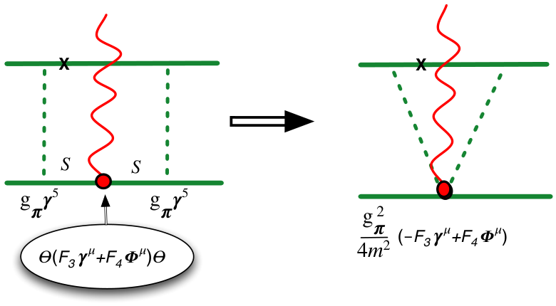
This correspondence mirrors that shown in Fig. 8 of Ref. I. In that case the off-shell sigma coupling cancelled the nucleon propagators. Here the details are very different, but the way in which off-shell projectors cancel propagators reducing the effective interaction of the off shell particle to a point interaction (modified by or ) is the same. It is another example of the theorem I proposed in Ref. I: a theory with off-shell couplings is equivalent to another theory with no off-shell couplings plus an infinite number of very complex interaction currents.
This comparison provides two further insights. First, I showed in Ref. I that the momentum dependent couplings in the kernel did not generate any two-pion exchange currents, while, as the example in Fig. 22 shows, the off-shell form factors do. Second, since the comparison suggests the physical role for is to generate two-pion exchange currents (as well as exchange currents involving other pairs of mesons) perhaps a more natural scale for the factor multiplying is (instead of which is merely a carry over from the factors multiplying ). If this were the case the form factor would be times smaller that the curves shown in Figs. 3 and 4. The new would be more comparable in size to .
VI.4 Outlook
I remind the reader that model VODG provides a very good explanation of the data for , and . However, the revised model IIB which is the basis of the VODG calculation, does not give a high precision fit to the data. The newer high precision fits provided by models WJC1 and WJC2, with their momentum dependent couplings and accompanying exchange currents, required a completely new calculation.
The fits to the off-shell form factors and the prediction of a new high behavior of completely fixes model WJC2, and allows for a precise prediction, without any free parameters, for the rescattering term in deuteron electrodisintegration at modest energy using the CST Adam:2002cn. In addition to being important in its own right, comparing this prediction to electrodisintegration data would be a decisive test of the CST.
Finally, extending the measurements of and particularly or to higher would yield new information about the off-shell deuteron form factors, and perhaps (in the absence of direct measurements) the neutron charge form factor . This paper provides the predictions with which to compare experimental results. Note in particular the CST prediction that will flatten out and reach a secondary maximum [recall Fig. (5)]. The large size of in this region may make measurements less difficult than previously anticipated.
Acknowledgements.
This work was partially supported by Jefferson Science Associates, LLC, under U.S. DOE Contract No. DE-AC05- 06OR23177. I especially want to thank Ingo Sick for sharing his Global Analysis (GA), without which it would have been more difficult to complete this work. It is also a pleasure to thank my colleagues for their support and collaboration over the years. In particular, I thank J. W. Van Orden, Alfred Stadler, and Carl Carlson for their significant contributions to the development of the CST as applied to scattering, and to previous calculations of the deuteron form factors.Appendix A Short review of the theory
This Appendix reviews some details of the calculations of the deuteron form factors discussed in several previous papers, but also includes some new analysis useful for a detailed understanding of this paper.
A.1 Form factors and helicity amplitudes
The most general form of the covariant deuteron electromagnetic vector current illustrated in Figs 1 and 2 can be expressed in terms of three deuteron form factors
| (48) |
where the form factors , , and are all functions of the square of the momentum transfer , with , , and () are the four-vector polarizations of the incoming (outgoing) deuterons with helicities (). The polarization vectors satisfy the well known constraints
| (49) |
This notation agrees with that used in Ref. Gilman:2001yh, except that now denotes the helicity of the outgoing deuteron and the helicity of the incoming deuteron.
The form factors and are usually replaced by the charge and quadrupole form factors, defined by
| (50) |
with defined in Eq. (23). At , the three form factors , , and give the charge, quadrupole moment, and magnetic moment of the deuteron
Contracting the vector current (48) with the photon helicity vectors
| (55) |
gives the helicity amplitudes, denoted by
| (56) |
The properties of the helicity amplitudes are discussed in Sec. III of Ref. II, where it was shown that only three of the possible 27 amplitudes are independent, so the form factors can be expressed in terms of the three combinations
| (57) |
where the symmetrised sum in the definition of is used for convenience. To calculate the deuteron form factors, it therefore sufficient to calculate the (with ).
A.2 Mathematical form of the current
The helicity amplitudes of the current, , are the sum of the three types of contributions shown in Fig. 2
| (58) |
The and contributions were combined in Eq. (3.28) of Ref. II; here I find it convenient to write them as two separate terms. Including the (B) diagrams from Eq. (3.36) of Ref. II, all three contributions can be written in a compact form:
| (59a) | |||||
| (59b) | |||||
| (59c) | |||||
where the integral is
| (60) |
the operator , with the phase , and , where was defined in Eq. (5). The coefficient of the term in Eq. (59a) differs from that reported in Ref. II; in includes a sum over two off-shell nucleon form factors, and , defined in Eq. (13). The quantities and are traces over products of pairs of covariant wave functions (or vertex functions), summarized in Table 7, one for the initial and one for the final deuteron, and are multiplied by one of the four from factors describing the interaction of the virtual photon with the off-shell nucleon. The detailed formulae for these traces are given in Ref. II: Eqs. (B1) and (B2) for , Eqs. (B6) and (B7) for , and Eqs. (B9) and (B10) for . I found corrections to these formulae that are reported in Appendix G.
The three types of wave functions or vertex functions that enter into the traces (59a) – (59c) are , and . The equation for the bound state wave function with particle 1 on shell is
| (61) |
where is the symmetrized one boson exchange (OBE) kernel (introduced in Ref. Gross:2008ps and discussed in detail in Ref. I) and the volume integral was defined in (60). The wave function and the subtracted vertex function (where can be off-shell) are obtained from an iteration of the basic equation (61) using the kernels and
| (62a) | ||||
| (62b) | ||||
where and are kernels constructed from the momentum dependence of the meson- vertiex couplings to particle 1 and 2 as described in Ref. I.
The off-shell subtracted vertex function is composed of two parts with a different matrix structure. These were previously defined in Eq. (41). The B part of the vertex function appears in the traces and the C part in the traces. (The reader is warned not to confuse the B term in Eq. (41) with the total contribution to the (B) diagrams.) Note that each of the trace terms is singular when , and only through the cancellation of the two terms at is this singularity removed. This cancellation is required by the physical behavior of this contribution, as discussed in detail in Sec. IIF of Ref. I. The C term vanishes when particle 1 is on-shell, and is interesting because it is a measure of contributions from off-shell terms that do not contribute to the on-shell two-body CST equation used to fix the parameters of the kernel.
A.3 Relativistic effects due to shifts in the arguments of the wave functions
The wave functions and vertex functions (referred to collectively as wave functions in the following discussion) that enter into the relativistic formulae have arguments shifted by the relativistic kinematics. It is of considerable interest in itself to study the size of these affects, and this is the focus of this subsection.
A.3.1 Arguments for the A diagrams
As discussed in Sec. IIC of Ref. II, when one particle is on-shell, the wave functions depend on only one variable, which I have chosen to be (the square of the three momentum of the on-shell particle 1). When boosted to the rest frame, this variable is denoted by , which is then either the momentum of particle 1 or the relative momentum of both particles (identical in the rest frame). The quantity is a function of , (the component of in the direction of ), and .
For the A diagrams, with the momenta labeled as in Fig. 1(A), the exact expression for this argument is [using for rest frame values from diagram (A)]
| (63a) | |||||
| (63b) | |||||
| (63c) | |||||
where [] is the rest frame value of obtained from a moving incoming (outgoing) deuteron in the Breit frame.
The last expression, Eq. (63c), is the value of the rest frame momentum in the infinite mass (nonrelativistic) limit, and shows that, nonrelativistically, these momenta must be interpreted as the relative momenta, , because before and after the collision with the photon, the assignment of momenta that correctly describes this process is
| (64) |
Note the reassuring fact that Eq. (63a) gives the same result if is replaced by the relative momentum in the moving frame
| (65) | |||||
The lesson from this discussion is that the effective rest frame momentum, , is the same whether or not one starts in the moving frame from the four-momentum of particle 1, or the relative four-momentum of the two particles; this must be true, of course, since the two are indistinguishable in the rest system.
To better understand the results (63b) and (63c), it is useful to obtain the longitudinal and transverse components of by directly transforming the components of from the moving system to the rest system, using the relations
| (66) |
where it is easily shown that . In Fig. 23 I show the related components
| (67) |
plotted in the plane.
Two cases are shown in the figure. The first is the nonrelativistic limit of the boost (with ). It is described by the dashed black circle which can be described as the locus of points swept out by the unit vector (represented by the dashed arrow fixed to the origin) rotating through polar angle with the axis. However, the same circle is also the locus of points swept out by , represented by the longer black dashed vector, with one end fixed at the reference point (represented by the round black dot at in the figure) and the other end following the locus of points swept out by dashed circle. This vector, which is the rest frame momentum in the nonrelativistic limit, divide by , must change length in order to track the dashed circle.
The second case shown is the solid red ellipse, which shows the behavior of the relativistic A-type rest-frame momentum. Because ( for the parameters chosen) the curve changes from a circle to an ellipse and the reference point (represented by the solid red square) shifts to . The vector that sweeps out the relativistic momentum is represented by the red arrow that connects the solid red square reference point to the ellipse. One can see clearly how the relativistic transformation changes the effective rest-frame momentum; the shift in the reference point is due to the role that the particle energy plays in the transformation, and change from a circle to an ellipse is due to the dilation factor in the transformation.
Fig. 23 shows the relativistic ellipse expanding in the direction, rather than contracting. This is because we are keeping constant in the moving frame. To obtain this condition, we must start from an expanded ellipse in the rest-frame, so that when it is contracted by the transformation to the moving system it will be compressed back into a circle. Hence the transformation behaves as expected after all. This expansion explains qualitatively the behavior of the relativistic argument shift shown by the dashed blue line shown in Fig. 20.
A.3.2 Arguments for the B diagrams
For the B diagrams, when both particles can be off-shell, the wave functions can depend on an additional variable, which was previously chosen to be the energy of particle 1 in the moving frame, , which transformed to in the rest frame. The momenta are labeled in Fig. 2(B) and following the discussion in Sec. III.3, I make the substitution
| (68) |
into the momenta given in Ref. II (with the change in notation )
| (69) | |||||
where [recalling that the momenta in Fig. 2(B) are labeled with a tilda to distinguish them from momenta in Fig. 2(A)]
| (70) |
I prefer using the variable instead of the unconstrained energy because when particle 1 is on-shell, , independent of momenta. Hence
| (71) | |||||
It is easy to see that is constrained by the mass shell condition
| (72) |
as required by relativity. The condition is now a simple, momentum independent way to specify that particle 1 is on-shell.
In the calculation of the (B) diagram, only the values of given in Eq. (37) are needed. To order these are
| (73) | |||||
When this is substituted into (69), the result to order is
| (74) | |||||
showing that the mass shell condition holds to order .
While is the appropriate quantity describing the off-shell behavior in the moving frame, the quantity that describes this in the rest frame of each state, denoted by , is defined by the relations
| (75) |
This can be derived directly by transforming and in Eq. (68) to the rest frame and requiring the transformation of to maintain the equation. Note that setting in (75) and using the relation (72) gives the result .
It is satisfying to observe that nonrelativistic limits of the momenta (69) [or (71)] correctly describe the process in which the photon is absorption on particle 1 instead of particle 2:
| (76) |
This is a consequence of the fact that the nonrelativistic limit of is not equal to .
As I did in the previous subsection, it is useful to derive (69) directly from the Lorentz boost. Starting from the off-shell four-momentum of particle 1 in the moving frame, (where pairs with momenta ), and transforming to the rest frame using , gives
| (77) |
This result for agrees immediately with (69), and it is also easy to show that as expected.
To represent the behavior of the spacial components when particle 1 is on shell, Fig. 24 shows the behavior of the two components that enter into the (B+) diagram when
| (78) | |||||
In defining , I introduced a new subtraction term depending on the energy ,
| (79) |
chosen to be independent of and of the correct size to center the elliptical locus of the points at the origin
The solid red ellipse shown in Fig. 24 is the locus of points swept out by the vector , which reaches from the new reference point (the subtraction term) shown as a solid red diamond located on the axis at (for the same values GeV and MeV used in Fig. 23) to the smaller of the red ellipses, and has a different length than the one for diagram (A). For comparison, the ellipse for the transformation of diagram (A) shown in Fig. 23 is the red dashed ellipse in Fig. 24. The Lorentz transformation of the (A) and (B) diagrams have very different behaviors, which can be traced to the different behavior of the energies of particle 1 in the two cases.
I return now to the issue of how far off-shell particle 1 is forced by the kinematics in the 2(B) diagrams. This was already addressed nonrelativistically in Sec. III.3 above. As I showed there, the relevant values of , denoted , were given in Eq. (37). The correct quantity is therefore
| (80) | |||||
The maximum of occurs when (I drop the tilde at this point), giving
| (81) |
where
| (82) |
As for the non-boosted case, the minimum is found by changing (or to ). Also, note that
| (83) |
which, once has been found, agrees with the result (38).
For each , this limiting function is has a maximum at a particular value of (which is best found numerically) so the maximum and minimum for all can be shown as a function of only. This limiting value was already shown in Fig. 15. The figure shows how far off-shell the particle can be forced, even at modest values of .
A.4 Calculation of the off-shell invariant functions
The wave and vertex functions can be expanded into scalar functions. For recent discussion of the decomposition of , see Appendix A of Ref. II and Sec. III of Ref. Gross:2010qm. The wave function can be expressed in terms of four scalar functions: the two familiar nonrelativistic S and D-state wave functions, (S-state), (P-state), and the two small P-state components of relativistic origin, (spin triplet P-state), and (spin singlet P-state), or alternatively in terms of the helicity amplitudes (with ; see the discussion below). The momentum dependence of these wave functions was shown in Figs. 6 and 7 of Ref. Gross:2010qm.
In this subsection, I discuss a few technical details that I found helpful in carrying out the numerical calculations.
First, instead of using the amplitudes , where
| (84) |
I use the realted amplitudes
| (85) |
where and is related to the inverse of the nucleon propagator for positive and negative energy nucleon states. These propagators are
| (86) | |||||
The reason for using the ’s instead of the ’s is that the propagator appears naturally when the ’s are extended off-shell. Since is singular at , or at
| (87) |
the ’s are singular at these points, and it is hard to compute them numerically around these singularities. The problem becomes critical because these singularities are very close to at small . These singularities are cancelled in the amplitudes , which are very smooth near and provide a much better input for numerical solutions.
The eight invariant functions that define the Dirac-space form of the vertex function can be expressed in terms of the helicity amplitudes . The results in terms of the ’s was given in Eq. (A27) of Gross:2014wqa. When expressed in terms of the ’s the relations become
| (88) | |||||
where
| (89) |
with .
It turns out that only the four amplitudes need to be considered; the amplitudes will never contribute to the final result. The argument is in two steps. First, when particle 1 is on-shell, , and the four invariant functions do not depend on the amplitudes . Next, when both particles are off-shell, only subtracted amplitudes contribute, and I have found that the subtracted amplitudes are numerically so small as to be nearly zero, and can be discarded from the calculation. In this case the subtracted are not zero, but depend only on the amplitudes . I have not looked for a proof of the relation , which I believe to be true.
All of the invariants are regular as , yet the expressions for all but show a possible singularity at . To avoid this there must be relations between the ’s near . To examine this, drop all of the terms, and substitute and examine the limits, dropping all terms proportional to or higher, since they are finite. Taking , and using the expansions
| (90) |
gives
| (91) |
Requiring that these seven invariants be regular at gives conditions on the four vertex functions. Near , and independent of , we require
| (92) |
Note that these limits are satisfied by the usual behavior of the momentum space wave functions. Using the definitions [taken from (84) multiplied by ] gives
| (93) |
which shows that the standard behavior of the and state wave functions will satisfy the necessary conditions.
Appendix B Nonrelativistic form factor
B.1 Wave functions momentum space
To prepare for the discussion of the nonrelativistic form factor, I write the nonrelativistic wave functions in the form
| (94) |
where a generic name for the radial wave functions, or , and is the spherical harmonic with relations
| (95) |
Note that the wave functions in coordinate space are reduced and the wave functions in coordinate and momentum spaces are only distinguished is by their arguments ( for coordinate space and for momentum space). For a discussion of the phase , see Eq. (3.36) and the last paragraph of Sec. III C in Ref. Gross:2010qm. This phase, which comes from the familiar plane wave expansion, is need to keep the ’s real. The standard Fourier transform links the two spaces
| (96) |
Using the familiar plane wave expansion
| (97) | |||||
where is the spherical Bessel function, I reduce the Eqs. (96) to
| (98) |
Dropping the common factors gives the relations [see Eq. (A32) of Ref. II]
| (99) |
B.2 Derivation of the charge form factor in momentum space
The nonrelativistic charge form factor is
| (100) |
where . For convenience I give the derivation of the momentum space expression, which is not widely known.
Appendix C Extraction of and from data for and
Here I present details of how the unknown off-shell from factors and are determined from a simultaneous fit to the Sick GA “data” for and . To this end recall the expansion (19). Dropping explicit mention of the arguments, this expansion is rewritten in a form that isolates the and contributions
| (102) |
where is the value of form factor at each Sick GA point . A similar expansion for the parameter of Eq. (25) that fixes can be written
| (103) |
where
| (104) |
Solving Eqs. (102) (with ) and (103) (for and ) gives
| (105) |
were
| (106) |
Note that when , becomes
| (107) |
independent of the sign of , insuring that the are continuous at the point where .
Appendix D Extraction of from data for
While it is straightforward to extract the predicted values of from the data for , it is still useful to outline here the way in which this was done. I begin by isolating the contribution from the expansion (19). Dropping the arguments, the new expansion is
| (110) | |||||
where , is defined by the expression, and, as before, all nucleon form factors contributing to the deuteron are isoscalar, so that here . The first two on-shell nucleon form factors, and are related to the nucleon electric and magnetic form factors in the usual way
| (111) |
where . Hence
| (112) |
or, in terms of the calculated body form factors,
| (113) |
This defines all of the coefficients in the expansion (110).
| ’s | ||||
|---|---|---|---|---|
The quadratic dependence go on can now be expressed in a compact form
| (114) |
The coefficients (all functions of ) are
| (115) |
The solution to (114) is
| (116) |
where the sign of the square root was chosen to give a positive when .
The error in comes from both the error in and the errors in and . Since and contribute only to , its contribution to the error is contained in the factors
| (117) |
which contribute the following errors to the
| (118) |
combining these errors with the Experimental error in gives the following estimate for the error in
| (119) |
With these results in hand, we find the solution for from the solution for by subtracting , which is also assumed to have no error. Hence as given in (119).
Appendix E Redefinitions of the traces
In Refs. II and III the arguments for the and traces were chosen differently. This is inconvenient for the numerical calculations performed in this paper, and can be easily avoided by some redefinitions. Specializing to the case when the outgoing particle 1 is on-shell, momenta used for the were
| (120) |
while for the traces I previously used
| (121) |
where here, to avoid confusion, I labeled the momenta used for the diagrams by , and therefore in these expressions . The momenta can be transformed into the momenta by the simple transformation
| (122) |
In this Appendix I show the effect of this transformation on the formulae for the traces published in Ref. II.
First, consider the argument shifts for the traces. In Ref. II the arguments of the are shifted to
| (123) |
while the argument of the outgoing generic on-shell is
| (124) | |||||
If the outgoing state in the traces has particle 1 on shell, so that , these expressions are identical to the argument shifts given in Eq. (69), showing that the transformation (122) transforms the shifts for into those for .
The expressions for the traces depend on the coefficients defined in Table IX of Ref. II (some of which are defined in Tables VI and VII of that reference). The only coefficients that depend on are the ’s, with transformations summarized in Table 15, and the coefficients , , and the particle 1 momentum squared, , all of which transform to
| (125) | |||||
Finally, the volume integral transforms to
| (126) |
where in the final expression, I return to the definition used everywhere.
With these substitutions, the same four-vector is used for both the and traces.
Appendix F Corrected treatment of the angular integrals when
Evaluation of the he angular integrals was discussed in detail in Appendix B of Ref. Gross:2010qm, but the discussion there was not accurate for cases when . In that paper we introduced the variable to scale for the off-shell energy dependence to the relative energy, where
| (127) |
(c.f. Eq. (A16) of Ref. Gross:2010qm). However, since the relative energy can be large when , the quantity defined in this way can also become quite large, making numerical calculations using this quantity difficult to carry out accurately. In this paper I have chosen to scale the off-shell energy of particle 1, using the relation
| (128) |
It follows immediately that the relative energy, expressed in tin terms of is
| (129) |
so that
| (130) |
This correspondence can be used quite successfully in many places, but for the discussion of the angular integrals it is best to work directly with .
As an example, consider how the treatment of the direct terms must be modified when the both nucleons are off-shell. Now the the momentum transfer depends on
| (131) | |||||
where I assume that the initial state (with momentum ) has particle 1 on-shell. This momentum transfer is zero at the critical cosine
| (132) |
The angular integrals are strongly peaked at . When , and approaches 1 only when . This singularity can be handled by the methods used in Ref. Gross:2010qm. However, for , can be less than 1 and the angular integrals can peak inside of the region of integration. This requires a mapping of the type used for the exchange terms, described in Appendix B3, Eq. (B9) of Ref. Gross:2010qm.
Appendix G Errata in Ref. II
There are errors in the magnetic moment results reported in Ref. II. As I did in Ref. II, here I present the difference between the expansion of the relativistic calculation and to obtain the “corrections” to the magnetic moment coming from the relativistic calculation. Multiplying the normalization condition by 0.880, written in the form (approximating and in the terms)
| (133) | |||||
and subtracting this from the predictions of the (A) + (A(2)) + (B) diagrams (multiplied by 1/2) gives the following corrections to the magnetic moment
| (134) |
where the expression reflects the fact that the only nonzero contributions to come from the (B) [(A)(2))] diagrams and , while not zero, is of lower order and can be dropped. The non-zero contributions are therefore
| (135) |
Combining these terms allows us to compare then with Eq. (5.6) of Ref. II. The sums (divided by 2) are
| (136) |
Note that , and agree with Ref. II, but the others do not. The terms have been found to be negligible and were not recalculated.
In the process of computing the form factors, the following errata we discovered in the equations reported in Ref. II:
- 1.
Eq. (C3) should read
- 2.
Eq. (B1):
- •
the coefficient of the term should be divided by an additional factor of
- •
the coefficient of the term should be divided by an additional factor of
- •
- 3.
Eq. (B2):
- •
in the coefficient of , the term should be replaced by
- •
a closing parentheses, ), is missing from the coefficient of the term; it belongs just before , so that the coefficient of includes the and terms but not the term
- •
a similar closing parentheses, ), is missing from the coefficient of the term; it belongs just before
- •
in the coefficient of , the coefficient of is , and NOT
- •
- 4.
Eq. (B.7):
- •
the terms are divided by (not )
- •
in the coefficient of the term replace by and in the coefficient of the term replace by
- •
- 5.
Eq. (B10):
- •
the terms should be divided by
- •
divide the entire trace by an extra factor of (so the coefficient in front is , not
- •
These errors arose when the original Mathematica formula were transcribed into text. Fortunately, all of the results of Refs. II and III are unaffected by these errors because they were derived directly from the correct Mathematica formula.
References
- (1) F. Gross, “Covariant Spectator Theory of np scattering: Isoscalar interaction currents,” Phys. Rev. C 89, no. 6, 064001 (2014). Referred to as Ref. I.
- (2) F. Gross, “Covariant Spectator Theory of np scattering: Deuteron magnetic moment” Phys. Rev. C 89, no. 6, 064002 (2014). Referred to as Ref. II.
- (3) F. Gross, “Covariant Spectator Theory of np scattering: Deuteron Quadrupole Moment” Phys. Rev. C 91, no. 1, 014005 (2015). Referred to as Ref. III.
- (4) F. Gross, “Three-dimensional covariant integral equations for low-energy systems,” Phys. Rev. 186, 1448 (1969).
- (5) F. Gross, “A New Theory of Nuclear Forces. 1. Relativistic Origin of the Repulsive Core,” Phys. Rev. D 10, 223 (1974).
- (6) F. Gross, “The Relativistic Few Body Problem. 1. Two-Body Equations,” Phys. Rev. C 26, 2203 (1982).
- (7) J. W. Van Orden, N. Devine and F. Gross, Phys. Rev. Lett. 75, 4369 (1995). doi:10.1103/PhysRevLett.75.4369
- (8) F. Gross, J. W. Van Orden and K. Holinde, Phys. Rev. C 45, 2094 (1992).
- (9) M. Garcon and J. W. Van Orden, Adv. Nucl. Phys. 26, 293 (2001) [nucl-th/0102049].
- (10) R. A. Gilman and F. Gross, J. Phys. G 28, R37 (2002).
- (11) L. E. Marcucci et al., J. Phys. G 43, 023002 (2016) doi:10.1088/0954-3899/43/2/023002 [arXiv:1504.05063 [nucl-th]].
- (12) M. T. Pena, F. Gross and Y. Surya, Phys. Rev. C 54, 2235 (1996) doi:10.1103/PhysRevC.54.2235 [nucl-th/9605041].
- (13) F. Gross and A. Stadler, “Covariant spectator theory of np scattering: Phase shifts obtained from Phys. Rev. C 78, 014005 (2008).
- (14) F. Gross and A. Stadler, “Covariant spectator theory of scattering: Effective range expansions and relativistic deuteron wave functions,” Phys. Rev. C 82, 034004 (2010)
- (15) A. Stadler and F. Gross, Phys. Rev. Lett. 78, 26 (1997) doi:10.1103/PhysRevLett.78.26 [nucl-th/9607012].
- (16) F. Gross and D. O. Riska, Phys. Rev. C 36, 1928 (1987).
- (17) I. Sick, Prog. Part. Nucl. Phys. 47, 245 (2001), and private communication
- (18) E. L. Lomon, Phys. Rev. C 66, 045501 (2002) doi:10.1103/PhysRevC.66.045501 [nucl-th/0203081].
- (19) F. Cardarelli, I. L. Grach, I. Narodetsky, G. Salme and S. Simula, Phys. Lett. B 359, 1 (1995) doi:10.1016/0370-2693(95)01058-X [nucl-th/9509004].
- (20) C. D. Buchanan and M. R. Yearian, Phys. Rev. Lett. 15, 303 (1965).
- (21) G. G. Simon, C. Schmitt and V. H. Walther, Nucl. Phys. A 364, 285 (1981).
- (22) S. Auffret et al., Phys. Rev. Lett. 54, 649 (1985).
- (23) R. Cramer et al., Z. Phys. C 29, 513 (1985).
- (24) R. G. Arnold et al., Phys. Rev. Lett. 58, 1723 (1987).
- (25) P. E. Bosted et al., Phys. Rev. C 42, 38 (1990).
- (26) R. Suleiman, Measurements of the Electric and Magnetic Elastic Structure Functions of the Deuteron at Large Momentum Transfers, Ph.D. Thesis, Kent State University, December 1999.
- (27) G. G. Petratos, Nucl. Phys. A 663, 357 (2000).
- (28) M. E. Schulze et al., Phys. Rev. Lett. 52, 597 (1984). doi:10.1103/PhysRevLett.52.597
- (29) V. F. Dmitriev et al., Phys. Lett. 157B, 143 (1985). doi:10.1016/0370-2693(85)91534-5
- (30) B. B. Wojtsekhowski B B et al., JETP Lett. 43 733 (1986)
- (31) R. A. Gilman et al., Phys. Rev. Lett. 65, 1733 (1990). doi:10.1103/PhysRevLett.65.1733
- (32) B. Boden et al., Z. Phys. C 49, 175 (1991). doi:10.1007/BF01555492
- (33) I. The et al., Phys. Rev. Lett. 67, 173 (1991). doi:10.1103/PhysRevLett.67.173
- (34) M. Garcon et al., Phys. Rev. C 49, 2516 (1994). doi:10.1103/PhysRevC.49.2516
- (35) M. Ferro-Luzzi et al., Phys. Rev. Lett. 77, 2630 (1996). doi:10.1103/PhysRevLett.77.2630
- (36) M. Bouwhuis et al., Phys. Rev. Lett. 82, 3755 (1999) doi:10.1103/PhysRevLett.82.3755 [nucl-ex/9810004].
- (37) D. Abbott et al. [JLAB t(20) Collaboration], Phys. Rev. Lett. 84, 5053 (2000) doi:10.1103/PhysRevLett.84.5053 [nucl-ex/0001006].
- (38) D. M. Nikolenko et al., Nucl. Phys. A 684, 525 (2001). doi:10.1016/S0375-9474(01)00373-6
- (39) C. Zhang et al., Phys. Rev. Lett. 107, 252501 (2011). doi:10.1103/PhysRevLett.107.252501
- (40) D. Benaksas, D. Drickey and D. Frerejacque, Phys. Rev. 148, 1327 (1966). doi:10.1103/PhysRev.148.1327
- (41) J. E. Elias, J. I. Friedman, G. C. Hartmann, H. W. Kendall, P. N. Kirk, M. R. Sogard, L. P. Van Speybroeck and J. K. De Pagter, Phys. Rev. 177, 2075 (1969). doi:10.1103/PhysRev.177.2075
- (42) S. Galster, H. Klein, J. Moritz, K. H. Schmidt, D. Wegener and J. Bleckwenn, Nucl. Phys. B 32, 221 (1971). doi:10.1016/0550-3213(71)90068-X
- (43) R. G. Arnold et al., Phys. Rev. Lett. 35, 776 (1975). doi:10.1103/PhysRevLett.35.776
- (44) S. Platchkov et al., Nucl. Phys. A 510, 740 (1990). doi:10.1016/0375-9474(90)90358-S
- (45) L. C. Alexa et al. [Jefferson Lab Hall A Collaboration], Phys. Rev. Lett. 82, 1374 (1999) doi:10.1103/PhysRevLett.82.1374 [nucl-ex/9812002].
- (46) D. Abbott et al. [Jefferson Lab t(20) Collaboration], Phys. Rev. Lett. 82, 1379 (1999) doi:10.1103/PhysRevLett.82.1379 [nucl-ex/9810017].
- (47) T. Eden et al., Phys. Rev. C 50, no. 4, R1749 (1994). doi:10.1103/PhysRevC.50.R1749
- (48) C. Herberg et al., Eur. Phys. J. A 5, 131 (1999). doi:10.1007/s100500050268
- (49) M. Ostrick et al., Phys. Rev. Lett. 83, 276 (1999). doi:10.1103/PhysRevLett.83.276
- (50) D. I. Glazier et al., Eur. Phys. J. A 24, 101 (2005) doi:10.1140/epja/i2004-10115-8 [nucl-ex/0410026].
- (51) R. Madey et al. [E93-038 Collaboration], Phys. Rev. Lett. 91, 122002 (2003) doi:10.1103/PhysRevLett.91.122002 [nucl-ex/0308007].
- (52) B. Plaster et al. [Jefferson Laboratory E93-038 Collaboration], Phys. Rev. C 73, 025205 (2006) doi:10.1103/PhysRevC.73.025205 [nucl-ex/0511025].
- (53) I. Passchier et al., Phys. Rev. Lett. 82, 4988 (1999) doi:10.1103/PhysRevLett.82.4988 [nucl-ex/9907012].
- (54) H. Zhu et al. [E93026 Collaboration], Phys. Rev. Lett. 87, 081801 (2001) doi:10.1103/PhysRevLett.87.081801 [nucl-ex/0105001].
- (55) G. Warren et al. [Jefferson Lab E93-026 Collaboration], Phys. Rev. Lett. 92, 042301 (2004) doi:10.1103/PhysRevLett.92.042301 [nucl-ex/0308021].
- (56) C. F. Perdrisat, V. Punjabi and M. Vanderhaeghen, Prog. Part. Nucl. Phys. 59, 694 (2007) doi:10.1016/j.ppnp.2007.05.001 [hep-ph/0612014].
- (57) F. Gross, Phys. Rev. C 26, 2226 (1982). doi:10.1103/PhysRevC.26.2226
- (58) A. Stadler and F. Gross, AIP Conf. Proc. 334, 867 (1995). doi:10.1063/1.48120
- (59) A. Stadler, F. Gross and M. Frank, Phys. Rev. C 56, 2396 (1997) doi:10.1103/PhysRevC.56.2396 [nucl-th/9703043].
- (60) S. A. Pinto, A. Stadler and F. Gross, Phys. Rev. C 79, 054006 (2009) doi:10.1103/PhysRevC.79.054006 [arXiv:0901.4313 [nucl-th]].
- (61) S. A. Pinto, A. Stadler and F. Gross, Phys. Rev. C 81, 014007 (2010) doi:10.1103/PhysRevC.81.014007 [arXiv:0911.1473 [nucl-th]].
- (62) B. M. Casper and F. Gross, Phys. Rev. 155, 1607 (1967).
- (63) I. Sick and D. Trautmann, Nucl. Phys. A 637, 559 (1998). doi:10.1016/S0375-9474(98)00334-0
- (64) J. Adam, Jr., F. Gross, S. Jeschonnek, P. Ulmer and J. W. Van Orden, Phys. Rev. C 66, 044003 (2002) [nucl-th/0204068].