Theoretical Issues in Deep Networks: Approximation, Optimization and GeneralizationDOI: www.pnas.org/cgi/doi/10.1073/pnas.XXXXXXXXXX

We start with the first set of questions, summarizing results in HierarchicalKernels2015; Hierarchical2015; poggio2015December, and Mhaskaretal2016; MhaskarPoggio2016. The main result is that deep networks have the theoretical guarantee, which shallow networks do not have, that they can avoid the curse of dimensionality for an important class of problems, corresponding to compositional functions, that is functions of functions. An especially interesting subset of such compositional functions are hierarchically local compositional functions where all the constituent functions are local in the sense of bounded small dimensionality. The deep networks that can approximate them without the curse of dimensionality are of the deep convolutional type – though, importantly, weight sharing is not necessary.

Implications of the theorems likely to be relevant in practice are:

a) Deep convolutional architectures have the theoretical guarantee that they can be much better than one layer architectures such as kernel machines for certain classes of problems; b) the problems for which certain deep networks are guaranteed to avoid the curse of dimensionality (see for a nice review Donoho00high-dimensionaldata) correspond to input-output mappings that are compositional with local constituent functions; c) the key aspect of convolutional networks that can give them an exponential advantage is not weight sharing but locality at each level of the hierarchy.

Several papers in the ’80s focused on the approximation power and learning properties of one-hidden layer networks (called shallow networks here). Very little appeared on multilayer networks, (but see mhaskar1993approx; mhaskar1993neural; chui1994neural; chui1996; Pinkus1999). By now, several papers poggio03mathematics; MontufarBengio2014; DBLP:journals/corr/abs-1304-7045 have appeared. Anselmi2014; anselmi2015theoretical; poggioetal2015; LiaoPoggio2016; Mhaskaretal2016 derive new upper bounds for the approximation by deep networks of certain important classes of functions which avoid the curse of dimensionality. The upper bound for the approximation by shallow networks of general functions was well known to be exponential. It seems natural to assume that, since there is no general way for shallow networks to exploit a compositional prior, lower bounds for the approximation by shallow networks of compositional functions should also be exponential. In fact, examples of specific functions that cannot be represented efficiently by shallow networks have been given, for instance in Telgarsky2015; SafranShamir2016; Theory_I. An interesting review of approximation of univariate functions by deep networks has recently appeared 2019arXiv190502199D.

The general paradigm is as follows. We are interested in determining how complex a network ought to be to theoretically guarantee approximation of an unknown target function $f$ up to a given accuracy $\epsilon>0$. To measure the accuracy, we need a norm $\|\cdot\|$ on some normed linear space $\mathbb{X}$. As we will see the norm used in the results of this paper is the $sup$ norm in keeping with the standard choice in approximation theory. As it turns out, the results of this section require the sup norm in order to be independent from the unknown distribution of the input data.

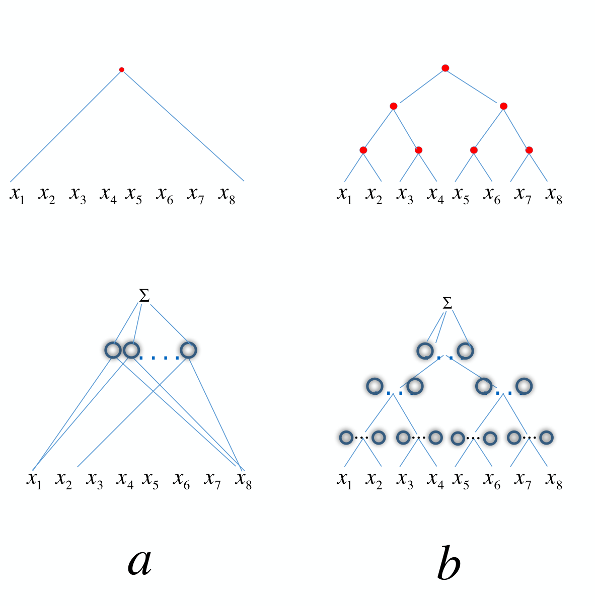
Let $V_{N}$ be the be set of all networks of a given kind with $N$ units (which we take to be or measure of the complexity of the approximant network). The degree of approximation is defined by $\mathsf{dist}(f,V_{N})=\inf_{P\in V_{N}}\|f-P\|.$ For example, if $\mathsf{dist}(f,V_{N})=\mathcal{O}(N^{-\gamma})$ for some $\gamma>0$, then a network with complexity $N=\mathcal{O}(\epsilon^{-\frac{1}{\gamma}})$ will be sufficient to guarantee an approximation with accuracy at least $\epsilon$. The only a priori information on the class of target functions $f$, is codified by the statement that $f\in W$ for some subspace $W\subseteq\mathbb{X}$. This subspace is a smoothness and compositional class, characterized by the parameters $m$ and $d$ ($d=2$ in the example of Figure 1 ; it is the size of the kernel in a convolutional network).

This section characterizes conditions under which deep networks are “better” than shallow network in approximating functions. Thus we compare shallow (one-hidden layer) networks with deep networks as shown in Figure 1. Both types of networks use the same small set of operations – dot products, linear combinations, a fixed nonlinear function of one variable, possibly convolution and pooling. Each node in the networks corresponds to a node in the graph of the function to be approximated, as shown in the Figure. A unit is a neuron which computes $(\left\langle{x},{w}\right\rangle+b)_{+}$, where $w$ is the vector of weights on the vector input $x$. Both $w$ and the real number $b$ are parameters tuned by learning. We assume here that each node in the networks computes the linear combination of $r$ such units $\sum_{i=1}^{r}c_{i}(\left\langle{x},{w_{i}}\right\rangle+b_{i})_{+}$. Notice that in our main example of a network corresponding to a function with a binary tree graph, the resulting architecture is an idealized version of deep convolutional neural networks described in the literature. In particular, it has only one output at the top unlike most of the deep architectures with many channels and many top-level outputs. Correspondingly, each node computes a single value instead of multiple channels, using the combination of several units. However our results hold also for these more complex networks (see Theory_I).

The sequence of results is as follows.

• •

  Both shallow (a) and deep (b) networks are universal, that is they can approximate arbitrarily well any continuous function of $n$ variables on a compact domain. The result for shallow networks is classical.

• •

  We consider a special class of functions of $n$ variables on a compact domain that are hierarchical compositions of local functions, such as $f(x_{1},\cdots,x_{8})=h_{3}(h_{21}(h_{11}(x_{1},x_{2}),h_{12}(x_{3},x_{4})),\allowbreak h_{22}(h_{13}(x_{5},x_{6}),h_{14}(x_{7},x_{8})))$

  The structure of the function in Figure 1 b) is represented by a graph of the binary tree type, reflecting dimensionality $d=2$ for the constituent functions $h$. In general, $d$ is arbitrary but fixed and independent of the dimensionality $n$ of the compositional function $f$. Theory_I formalizes the more general compositional case using directed acyclic graphs.

• •

  The approximation of functions with a compositional structure – can be achieved with the same degree of accuracy by deep and shallow networks but the number of parameters are much smaller for the deep networks than for the shallow network with equivalent approximation accuracy.

We approximate functions with networks in which the activation nonlinearity is a smoothed version of the so called ReLU, originally called ramp by Breiman and given by $\sigma(x)=x_{+}=max(0,x)$ . The architecture of the deep networks reflects the function graph with each node $h_{i}$ being a ridge function, comprising one or more neurons.

Let $I^{n}=[-1,1]^{n}$, $\mathbb{X}=C(I^{n})$ be the space of all continuous functions on $I^{n}$, with $\|f\|=\max_{x\in I^{n}}|f(x)|$. Let $\mathcal{S}_{N,n}$ denote the class of all shallow networks with $N$ units of the form

where ${w}_{k}\in\R^{n}$, $b_{k},a_{k}\in\R$. The number of trainable parameters here is $(n+2)N\sim n$. Let $m\geq 1$ be an integer, and $W_{m}^{n}$ be the set of all functions of $n$ variables with continuous partial derivatives of orders up to $m<\infty$ such that $\|f\|+\sum_{1\leq|\mathbf{k}|_{1}\leq m}\|D^{\mathbf{k}}f\|\leq 1$, where $D^{\mathbf{k}}$ denotes the partial derivative indicated by the multi-integer $\mathbf{k}\geq 1$, and $|\mathbf{k}|_{1}$ is the sum of the components of $\mathbf{k}$.

For the hierarchical binary tree network, the analogous spaces are defined by considering the compact set $W_{m}^{n,2}$ to be the class of all compositional functions $f$ of $n$ variables with a binary tree architecture and constituent functions $h$ in $W_{m}^{2}$. We define the corresponding class of deep networks $\mathcal{D}_{N,2}$ to be the set of all deep networks with a binary tree architecture, where each of the constituent nodes is in $\mathcal{S}_{M,2}$, where $N=|V|M$, $V$ being the set of non–leaf vertices of the tree. We note that in the case when $n$ is an integer power of $2$, the total number of parameters involved in a deep network in $\mathcal{D}_{N,2}$ is $4N$.

The first theorem is about shallow networks.

The estimate of Theorem 1 is the best possible if the only a priori information we are allowed to assume is that the target function belongs to $f\in W_{m}^{n}$. The exponential dependence on the dimension $n$ of the number $e^{-n/m}$ of parameters needed to obtain an accuracy $\mathcal{O}(\epsilon)$ is known as the curse of dimensionality. Note that the constants involved in $\mathcal{O}$ in the theorems will depend upon the norms of the derivatives of $f$ as well as $\sigma$.

Our second and main theorem is about deep networks with smooth activations (preliminary versions appeared in poggio2015December; Hierarchical2015; Mhaskaretal2016). We formulate it in the binary tree case for simplicity but it extends immediately to functions that are compositions of constituent functions of a fixed number of variables $d$ (in convolutional networks $d$ corresponds to the size of the kernel).

The proof is in Theory_I. The assumptions on $\sigma$ in the theorems are not satisfied by the ReLU function $x\mapsto x_{+}$, but they are satisfied by smoothing the function in an arbitrarily small interval around the origin. The result of the theorem can be extended to non-smooth ReLUTheory_I.

In summary, when the only a priori assumption on the target function is about the number of derivatives, then to guarantee an accuracy of $\epsilon$, we need a shallow network with $\mathcal{O}(\epsilon^{-n/m})$ trainable parameters. If we assume a hierarchical structure on the target function as in Theorem 2, then the corresponding deep network yields a guaranteed accuracy of $\epsilon$ with $\mathcal{O}(\epsilon^{-2/m})$ trainable parameters. Note that Theorem 2 applies to all $f$ with a compositional architecture given by a graph which correspond to, or is a subgraph of, the graph associated with the deep network – in this case the graph corresponding to $W_{m}^{n,d}$.

There are many recent papers studying optimization in deep learning. For optimization we mention work based on the idea that noisy gradient descent DBLP:journals/corr/Jin0NKJ17; DBLP:journals/corr/GeHJY15; pmlr-v49-lee16; s.2018when can find a global minimum. More recently, several authors studied the dynamics of gradient descent for deep networks with assumptions about the input distribution or on how the labels are generated. They obtain global convergence for some shallow neural networks Tian:2017:AFP:3305890.3306033; s8409482; Li:2017:CAT:3294771.3294828; DBLP:conf/icml/BrutzkusG17; pmlr-v80-du18b; DBLP:journals/corr/abs-1811-03804. Some local convergence results have also been proved Zhong:2017:RGO:3305890.3306109; DBLP:journals/corr/abs-1711-03440; 2018arXiv180607808Z. The most interesting such approach is DBLP:journals/corr/abs-1811-03804, which focuses on minimizing the training loss and proving that randomly initialized gradient descent can achieve zero training loss (see also NIPS2018_8038; du2018gradient; DBLP:journals/corr/abs-1811-08888). In summary, there is by now an extensive literature on optimization that formalizes and refines to different special cases and to the discrete domain our results of theory_II; theory_IIb.

The first part of the argument of this section relies on the obvious fact (see theory_III), that for RELU networks under the hypothesis of an exponential-type loss function, there are no local minima that separate the data – the only critical points of the gradient that separate the data are the global minima.

Notice that the global minima are at $\rho=\infty$, when the exponential is zero. As a consequence, the Hessian is identically zero with all eigenvalues being zero. On the other hand any point of the loss at a finite $\rho$ has nonzero Hessian: for instance in the linear case the Hessian is proportional to $\sum_{n}^{N}x_{n}x^{T}_{n}$. The local minima which are not global minima must misclassify. How degenerate are they?

Simple arguments theory_III suggest that the critical points which are not global minima cannot be completely degenerate. We thus have the following

For the general case of non-exponential loss and smooth nonlinearities instead of the RELU the following conjecture has been proposed theory_III:

The second part of our argument (in theory_IIb) is that SGD concentrates in probability on the most degenerate minima. The argument is based on the similarity between a Langevin equation and SGD and on the fact that the Boltzmann distribution is exactly the asymptotic “solution” of the stochastic differential Langevin equation and also of SGDL, defined as SGD with added white noise (see for instance raginskyetal17). The Boltzmann distribution is

Together theory_II and theory_III suggest the following

A number of papers have studied gradient descent for deep networks NIPS2017_6836; DBLP:journals/corr/abs-1811-04918; Arora2019FineGrainedAO. Close to the approach summarized here (details are in theory_III) is the paper Wei2018OnTM. Its authors study generalization assuming a regularizer because they are – like us – interested in normalized margin. Unlike their assumption of an explicit regularization, we show here that commonly used techniques, such as weight and batch normalization, in fact minimize the surrogate loss margin while controlling the complexity of the classifier without the need to add a regularizer or to use weight decay. Surprisingly, we will show that even standard gradient descent on the weights implicitly controls the complexity through an “implicit” unit $L_{2}$ norm constraint. Two very recent papers (2019arXiv190507325S and DBLP:journals/corr/abs-1906-05890) develop an elegant but complicated margin maximization based approach which lead to some of the same results of this section (and many more). The important question of which conditions are necessary for gradient descent to converge to the maximum of the margin of $\tilde{f}$ are studied by 2019arXiv190507325S and DBLP:journals/corr/abs-1906-05890. Our approach does not need the notion of maximum margin but our theorem 3 establishes a connection with it and thus with the results of 2019arXiv190507325S and DBLP:journals/corr/abs-1906-05890. Our main goal here (and in theory_III) is to achieve a simple understanding of where the complexity control underlying generalization is hiding in the training of deep networks.

We define a deep network with $K$ layers with the usual coordinate-wise scalar activation functions $\sigma(z):\quad\mathbf{R}\to\mathbf{R}$ as the set of functions $f(W;x)=\sigma(W^{K}\sigma(W^{K-1}\cdots\sigma(W^{1}x)))$, where the input is $x\in\mathbf{R}^{d}$, the weights are given by the matrices $W^{k}$, one per layer, with matching dimensions. We sometime use the symbol $W$ as a shorthand for the set of $W^{k}$ matrices $k=1,\cdots,K$. For simplicity we consider here the case of binary classification in which $f$ takes scalar values, implying that the last layer matrix $W^{K}$ is $W^{K}\in\mathbf{R}^{1,K_{l}}$. The labels are $y_{n}\in\{-1,1\}$. The weights of hidden layer $l$ are collected in a matrix of size $h_{l}\times h_{l-1}$. There are no biases apart form the input layer where the bias is instantiated by one of the input dimensions being a constant. The activation function in this section is the ReLU activation.

For ReLU activations the following important positive one-homogeneity property holds $\sigma(z)=\frac{\partial\sigma(z)}{\partial z}z$. A consequence of one-homogeneity is a structural lemma (Lemma 2.1 of DBLP:journals/corr/abs-1711-01530) $\sum_{i,j}W^{i,j}_{k}\left(\frac{\partial f(x)}{\partial W^{i,j}_{k}}\right)=f(x)$ where $W_{k}$ is here the vectorized representation of the weight matrices $W_{k}$ for each of the different layers (each matrix is a vector).

For the network, homogeneity implies $f(W;x)=\prod_{k=1}^{K}\rho_{k}f(V_{1},\cdots,V_{K};x_{n})$, where $W_{k}=\rho_{k}V_{k}$ with the matrix norm $||V_{k}||_{p}=1$. Another property of the Rademacher complexity of ReLU networks that follows from homogeneity is $\mathbb{R}_{N}(\mathbb{F})=\rho\mathbb{R}_{N}(\tilde{\mathbb{F}})$ where $\rho=\rho_{1}\prod_{k=1}^{K}\rho_{k}$, $\mathbb{F}$ is the class of neural networks described above.

We define $f=\rho\tilde{f}$; $\tilde{\mathbb{F}}$ is the associated class of normalized neural networks (we call $f(V;x)=\tilde{f}(x)$ with the understanding that $f(x)=f(W;x)$). Note that $\frac{\partial f}{\partial\rho_{k}}=\frac{\rho}{\rho_{k}}\tilde{f}$ and that the definitions of $\rho_{k}$, $V_{k}$ and $\tilde{f}$ all depend on the choice of the norm used in normalization.

In the case of training data that can be separated by the networks $f(x_{n})y_{n}>0\quad\forall n=1,\cdots,N$. We will sometime write $f(x_{n})$ as a shorthand for $y_{n}f(x_{n})$.

Classical generalization bounds for regression Bousquet2003 suggest that minimizing the empirical loss of a loss function such as the cross-entropy subject to constrained complexity of the minimizer is a way to to attain generalization, that is an expected loss which is close to the empirical loss:

Thus minimizing under a constraint on the Rademacher complexity a surrogate function such as the cross-entropy (which becomes the logistic loss in the binary classification case) will minimize an upper bound on the expected classification error because such surrogate functions are upper bounds on the $0-1$ function. We can choose a class of functions $\mathbf{\tilde{F}}$ with normalized weights and write $f(x)=\rho\tilde{f}(x)$ and $\mathbb{R}_{N}(\mathbb{F})=\rho\mathbb{R}_{N}(\mathbb{\tilde{F}})$. One can choose any fixed $\rho$ as a (Ivanov) regularization-type tradeoff.

In the following we explore the implications for deep networks of this classical approach to generalization.

The approach is then to minimize the loss function $L(f(w))=\sum_{n=1}^{N}e^{-f(W;x_{n})y_{n}}=\sum_{n=1}^{N}e^{-\rho f(V_{k};x_{n})y_{n}}$, with $\rho=\prod\rho_{k}$, subject to $||V_{k}||^{p}_{p}=1\ \forall k$, that is under a unit norm constraint for the weight matrix at each layer (if $p=2$ then $\sum_{i,j}(V_{k})_{i,j}^{2}=1$ is the Frobenius norm), since $V_{k}$ are the directions of the weights which are the relevant quantity for classification. The minimization is understood as a sequence of minimizations for a sequence of increasing $\rho_{k}$. Clearly these constraints imply the constraint on the norm of the product of weight matrices for any $p$ norm (because any induced operator norm is a sub-multiplicative matrix norm). The standard choice for a loss function is an exponential-type loss such the cross-entropy, which for binary classification becomes the logistic function. We study here the exponential because it is simpler and retains all the basic properties.

There are several gradient descent techniques that given the unconstrained optimization problem transform it into a constrained gradient descent problem. To provide the background let us formulate the standard unconstrained gradient descent problem for the exponential loss as it is used in practical training of deep networks:

The set of gradient-based algorithms enforcing a unit-norm constraints 845952 comprises several techniques that are equivalent for small values of the step size. They are all good approximations of the true gradient method. One of them is the Lagrange multiplier method; another is the tangent gradient method based on the following theorem:

In particular, a form for $g$ is $g(t)=\mu(t)\nabla_{u}L$, the gradient update in a gradient descent algorithm. We call $Sg(t)$ the tangent gradient transformation of $g$. In the case of $p=2$ we replace $\nu$ in Equation 8 with $u$ because $\nu(t)=\frac{\partial||u||_{2}}{\partial u}=u$. This gives $S=I-\frac{uu^{T}}{||u||_{2}^{2}}$ and $\dot{u}=Sg(t).$

Consider now the empirical loss $L$ written in terms of $V_{k}$ and $\rho_{k}$ instead of $W_{k}$, using the change of variables defined by $W_{k}=\rho_{k}V_{k}$ but without imposing a unit norm constraint on $V_{k}$. The flows in $\rho_{k},V_{k}$ can be computed as $\dot{\rho_{k}}=\frac{\partial W_{k}}{\partial\rho_{k}}\frac{\partial L}{\partial W_{k}}=V_{k}^{T}\frac{\partial L}{\partial W_{k}}$ and $\dot{V_{k}}=\frac{\partial W_{k}}{\partial V_{k}}\frac{\partial L}{\partial W_{k}}=\rho_{k}\frac{\partial L}{\partial W_{k}}$, with $\frac{\partial L}{\partial W_{k}}$ given by Equations 7.

We now enforce the unit norm constraint on $V_{k}$ by using the tangent gradient transform on the $V_{k}$ flow. This yields

Notice that the dynamics above follows from the classical approach of controlling the Rademacher complexity of $\tilde{f}$ during optimization (suggested by bounds such as Equation 4. The approach and the resulting dynamics for the directions of the weights may seem different from the standard unconstrained approach in training deep networks. It turns out, however, that the dynamics described by Equations 9 is the same dynamics of Weight Normalization.

It is easy to see that Equations 9 are the same as the weight normalization Equations 10, if $||v||_{2}=1$. We now observe, multiplying Equation 9 by $v^{T}$, that $v^{T}\dot{v}=0$ because $v^{T}S=0$, implying that $||v||^{2}$ is constant in time with a constant that can be taken to be $1$. Thus the two dynamics are the same.

Empirically it appears that GD and SGD converge to solutions that can generalize even without batch or weight normalization. Convergence may be difficult for quite deep networks and generalization may not be as good as with batch normalization but it still occurs. How is this possible?

We study the dynamical system $\dot{W_{k}}^{i,j}$ under the reparametrization $W^{i,j}_{k}=\rho_{k}V^{i,j}_{k}$ with $||V_{k}||_{2}=1$. We consider for each weight matrix $W_{k}$ the corresponding “vectorized” representation in terms of vectors $W_{k}^{i,j}=W_{k}$. We use the following definitions and properties (for a vector $w$):

• •

  Define $\frac{w}{||w||_{2}}=\tilde{w}$; thus $w=||w||_{2}\tilde{w}$ with $||\tilde{w}||_{2}=1$. Also define $S={I-\tilde{w}\tilde{w}^{T}}=I-\frac{ww^{T}}{||w||_{2}^{2}}$.

• •

  The following relations are easy to check:

  1. 1.

     $\frac{\partial||w||_{2}}{\partial w}=\tilde{w}$

  2. 2.

     $\frac{\partial\tilde{w}}{\partial w}=\frac{S}{||w||_{2}}$.

  3. 3.

     $Sw=S\tilde{w}=0$

  4. 4.

     $S^{2}=S$

The key point here is that the dynamics of $\dot{V_{k}}$ includes a unit $L_{2}$ norm constraint: using the tangent gradient transform will not change the equation because $S^{2}=S$.

As separate remarks , notice that if for $t>t_{0}$, $f$ separates all the data, $\frac{d}{dt}{\rho_{k}}>0$, that is $\rho$ diverges to $\infty$ with $\lim_{t\to\infty}\dot{\rho}=0$. In the 1-layer network case the dynamics yields $\rho\approx\log t$ asymptotically. For deeper networks, this is different. theory_III shows (for one support vector) that the product of weights at each layer diverges faster than logarithmically, but each individual layer diverges slower than in the 1-layer case. The norm of the each layer grows at the same rate $\dot{\rho_{k}^{2}}$, independent of $k$. The $V_{k}$ dynamics has stationary or critical points given by

To understand whether there exists an implicit complexity control in standard gradient descent of the weight directions, we check whether there exists an $L_{p}$ norm for which unconstrained normalization is equivalent to constrained normalization.

From Theorem 4 we expect the constrained case to be given by the action of the following projector onto the tangent space:

The constrained Gradient Descent is then

On the other hand, reparametrization of the unconstrained dynamics in the $p$-norm gives (following Equations 11 and 12)

These two dynamical systems are clearly different for generic $p$ reflecting the presence or absence of a regularization-like constraint on the dynamics of $V_{k}$.

As we have seen however, for $p=2$ the 1-layer dynamical system obtained by minimizing $L$ in $\rho_{k}$ and $V_{k}$ with $W_{k}=\rho_{k}V_{k}$ under the constraint $||V_{k}||_{2}=1$, is the weight normalization dynamics

The two dynamical systems differ only by a $\rho_{k}^{2}$ factor in the $\dot{V_{k}}$ equations. However, the critical points of the gradient for the $V_{k}$ flow, that is the point for which $\dot{V_{k}}=0$, are the same in both cases since for any $t>0$ $\rho_{k}(t)>0$ and thus $\dot{V_{k}}=0$ is equivalent to $S\dot{W_{k}}=0$. Hence, gradient descent with unit $L_{p}$-norm constraint is equivalent to the standard, unconstrained gradient descent but only when $p=2$. Thus

Thus standard GD implicitly enforces the $L_{2}$ norm constraint on $V_{k}=\frac{W_{k}}{||W_{k}||_{2}}$, consistently with Srebro’s results on implicit bias of GD. Other minimization techniques such as coordinate descent may be biased towards different norm constraints.

The linear ($f(x)=\rho v^{T}x$) networks case 2017arXiv171010345S is an interesting example of our analysis in terms of $\rho$ and $v$ dynamics. We start with unconstrained gradient descent, that is with the dynamical system

If gradient descent in $v$ converges to $\dot{v}=0$ at finite time, $v$ satisfies $vv^{T}x=x$, where $x=\sum_{j=1}^{C}\alpha_{j}x_{j}$ with positive coefficients $\alpha_{j}$ and $x_{j}$ are the $C$ support vectors (see theory_III). A solution $v^{T}=||x||x^{\dagger}$ then exists ($x^{\dagger}$, the pseudoinverse of $x$, since $x$ is a vector, is given by $x^{\dagger}=\frac{x^{T}}{||x||^{2}}$). On the other hand, the operator $T$ in $v(t+1)=Tv(t)$ associated with equation 19 is non-expanding, because $||v||=1,\ \forall t$. Thus there is a fixed point $v\propto x$ which is independent of initial conditions Ferreira1996 and unique (in the linear case)

A similar analysis for the weight normalization equations 17 considers the same dynamical system with a change in the equation for $v$, which becomes

This equation differs by a factor $\rho^{2}$ from equation 20. As a consequence equation 21 is of the form $\dot{\epsilon}=-\frac{\log t}{t}\epsilon$, with a general solution of the form $\epsilon\propto t^{-\frac{1}{2}\log t}$. In summary, GD with weight normalization converges faster to the same equilibrium than standard gradient descent: the rate for $\epsilon=v-x$ is $t^{-\frac{1}{2}log(t)}$ vs $\frac{1}{\log t}$.

Our goal was to find $\lim_{\rho\to\infty}\arg\min_{||V_{k}||=1,\ \forall k}L(\rho\tilde{f})$. We have seen that various forms of gradient descent enforce different paths in increasing $\rho$ that empirically have different effects on convergence rate. It will be an interesting theoretical and practical challenge to find the optimal way, in terms of generalization and convergence rate, to grow $\rho\rightarrow\infty$.

Our analysis of simplified batch normalization theory_III suggests that several of the same considerations that we used for weight normalization should apply (in the linear one layer case BN is identical to WN). However, BN differs from WN in the multilayer case in several ways, in addition to weight normalization: it has for instance separate normalization for each unit, that is for each row of the weight matrix at each layer.

References

- (1) Banburski A, et al. (2019) Theory of deep learning III: Dynamics and generalization in deep networks. CBMM Memo No. 090.
- (2) Soudry D, Hoffer E, Srebro N (2017) The Implicit Bias of Gradient Descent on Separable Data. ArXiv e-prints.
- (3) Lyu K, Li J (2019) Gradient descent maximizes the margin of homogeneous neural networks. CoRR abs/1906.05890.
- (4) Shpigel Nacson M, Gunasekar S, Lee JD, Srebro N, Soudry D (2019) Lexicographic and Depth-Sensitive Margins in Homogeneous and Non-Homogeneous Deep Models. arXiv e-prints p. arXiv:1905.07325.
- (5) Anselmi F, Rosasco L, Tan C, Poggio T (2015) Deep convolutional network are hierarchical kernel machines. Center for Brains, Minds and Machines (CBMM) Memo No. 35, also in arXiv.
- (6) Poggio T, Rosasco L, Shashua A, Cohen N, Anselmi F (2015) Notes on hierarchical splines, dclns and i-theory, (MIT Computer Science and Artificial Intelligence Laboratory), Technical report.
- (7) Poggio T, Anselmi F, Rosasco L (2015) I-theory on depth vs width: hierarchical function composition. CBMM memo 041.
- (8) Mhaskar H, Liao Q, Poggio T (2016) Learning real and boolean functions: When is deep better than shallow? Center for Brains, Minds and Machines (CBMM) Memo No. 45, also in arXiv.
- (9) Mhaskar H, Poggio T (2016) Deep versus shallow networks: an approximation theory perspective. Center for Brains, Minds and Machines (CBMM) Memo No. 54, also in arXiv.
- (10) Donoho DL (2000) High-dimensional data analysis: The curses and blessings of dimensionality in AMS CONFERENCE ON MATH CHALLENGES OF THE 21ST CENTURY.
- (11) Mhaskar H (1993) Approximation properties of a multilayered feedforward artificial neural network. Advances in Computational Mathematics pp. 61–80.
- (12) Mhaskar HN (1993) Neural networks for localized approximation of real functions in Neural Networks for Processing [1993] III. Proceedings of the 1993 IEEE-SP Workshop. (IEEE), pp. 190–196.
- (13) Chui C, Li X, Mhaskar H (1994) Neural networks for localized approximation. Mathematics of Computation 63(208):607–623.
- (14) Chui CK, Li X, Mhaskar HN (1996) Limitations of the approximation capabilities of neural networks with one hidden layer. Advances in Computational Mathematics 5(1):233–243.
- (15) Pinkus A (1999) Approximation theory of the mlp model in neural networks. Acta Numerica 8:143–195.
- (16) Poggio T, Smale S (2003) The mathematics of learning: Dealing with data. Notices of the American Mathematical Society (AMS) 50(5):537–544.
- (17) Montufar, G. F.and Pascanu R, Cho K, Bengio Y (2014) On the number of linear regions of deep neural networks. Advances in Neural Information Processing Systems 27:2924–2932.
- (18) Livni R, Shalev-Shwartz S, Shamir O (2013) A provably efficient algorithm for training deep networks. CoRR abs/1304.7045.
- (19) Anselmi F, et al. (2014) Unsupervised learning of invariant representations with low sample complexity: the magic of sensory cortex or a new framework for machine learning?. Center for Brains, Minds and Machines (CBMM) Memo No. 1. arXiv:1311.4158v5.
- (20) Anselmi F, et al. (2015) Unsupervised learning of invariant representations. Theoretical Computer Science.
- (21) Poggio T, Rosaco L, Shashua A, Cohen N, Anselmi F (2015) Notes on hierarchical splines, dclns and i-theory. CBMM memo 037.
- (22) Liao Q, Poggio T (2016) Bridging the gap between residual learning, recurrent neural networks and visual cortex. Center for Brains, Minds and Machines (CBMM) Memo No. 47, also in arXiv.
- (23) Telgarsky M (2015) Representation benefits of deep feedforward networks. arXiv preprint arXiv:1509.08101v2 [cs.LG] 29 Sep 2015.
- (24) Safran I, Shamir O (2016) Depth separation in relu networks for approximating smooth non-linear functions. arXiv:1610.09887v1.
- (25) Poggio T, Mhaskar H, Rosasco L, Miranda B, Liao Q (2016) Theory I: Why and when can deep - but not shallow - networks avoid the curse of dimensionality, (CBMM Memo No. 058, MIT Center for Brains, Minds and Machines), Technical report.
- (26) Daubechies I, DeVore R, Foucart S, Hanin B, Petrova G (2019) Nonlinear approximation and (deep) relu networks. arXiv e-prints p. arXiv:1905.02199.
- (27) Jin C, Ge R, Netrapalli P, Kakade SM, Jordan MI (2017) How to escape saddle points efficiently. CoRR abs/1703.00887.
- (28) Ge R, Huang F, Jin C, Yuan Y (2015) Escaping from saddle points - online stochastic gradient for tensor decomposition. CoRR abs/1503.02101.
- (29) Lee JD, Simchowitz M, Jordan MI, Recht B (2016) Gradient descent only converges to minimizers in 29th Annual Conference on Learning Theory, Proceedings of Machine Learning Research, eds. Feldman V, Rakhlin A, Shamir O. (PMLR, Columbia University, New York, New York, USA), Vol. 49, pp. 1246–1257.
- (30) Du SS, Lee JD, Tian Y (2018) When is a convolutional filter easy to learn? in International Conference on Learning Representations.
- (31) Tian Y (2017) An analytical formula of population gradient for two-layered relu network and its applications in convergence and critical point analysis in Proceedings of the 34th International Conference on Machine Learning - Volume 70, ICML’17. (JMLR.org), pp. 3404–3413.
- (32) Soltanolkotabi M, Javanmard A, Lee JD (2019) Theoretical insights into the optimization landscape of over-parameterized shallow neural networks. IEEE Transactions on Information Theory 65(2):742–769.
- (33) Li Y, Yuan Y (2017) Convergence analysis of two-layer neural networks with relu activation in Proceedings of the 31st International Conference on Neural Information Processing Systems, NIPS’17. (Curran Associates Inc., USA), pp. 597–607.
- (34) Brutzkus A, Globerson A (2017) Globally optimal gradient descent for a convnet with gaussian inputs in Proceedings of the 34th International Conference on Machine Learning, ICML 2017, Sydney, NSW, Australia, 6-11 August 2017. pp. 605–614.
- (35) Du S, Lee J, Tian Y, Singh A, Poczos B (2018) Gradient descent learns one-hidden-layer CNN: Don’t be afraid of spurious local minima in Proceedings of the 35th International Conference on Machine Learning, Proceedings of Machine Learning Research, eds. Dy J, Krause A. (PMLR, Stockholmsmässan, Stockholm Sweden), Vol. 80, pp. 1339–1348.
- (36) Du SS, Lee JD, Li H, Wang L, Zhai X (2018) Gradient descent finds global minima of deep neural networks. CoRR abs/1811.03804.
- (37) Zhong K, Song Z, Jain P, Bartlett PL, Dhillon IS (2017) Recovery guarantees for one-hidden-layer neural networks in Proceedings of the 34th International Conference on Machine Learning - Volume 70, ICML’17. (JMLR.org), pp. 4140–4149.
- (38) Zhong K, Song Z, Dhillon IS (2017) Learning non-overlapping convolutional neural networks with multiple kernels. CoRR abs/1711.03440.
- (39) Zhang X, Yu Y, Wang L, Gu Q (2018) Learning One-hidden-layer ReLU Networks via Gradient Descent. arXiv e-prints.
- (40) Li Y, Liang Y (2018) Learning overparameterized neural networks via stochastic gradient descent on structured data in Advances in Neural Information Processing Systems 31, eds. Bengio S, et al. (Curran Associates, Inc.), pp. 8157–8166.
- (41) Du SS, Zhai X, Poczos B, Singh A (2019) Gradient descent provably optimizes over-parameterized neural networks in International Conference on Learning Representations.
- (42) Zou D, Cao Y, Zhou D, Gu Q (2018) Stochastic gradient descent optimizes over-parameterized deep relu networks. CoRR abs/1811.08888.
- (43) Poggio T, Liao Q (2017) Theory II: Landscape of the empirical risk in deep learning. arXiv:1703.09833, CBMM Memo No. 066.
- (44) Zhang C, et al. (2017) Theory of deep learning IIb: Optimization properties of SGD. CBMM Memo 072.
- (45) Raginsky M, Rakhlin A, Telgarsky M (2017) Non-convex learning via stochastic gradient langevin dynamics: A nonasymptotic analysis. arXiv:180.3251 [cs, math].
- (46) Daniely A (2017) Sgd learns the conjugate kernel class of the network in Advances in Neural Information Processing Systems 30, eds. Guyon I, et al. (Curran Associates, Inc.), pp. 2422–2430.
- (47) Allen-Zhu Z, Li Y, Liang Y (2018) Learning and generalization in overparameterized neural networks, going beyond two layers. CoRR abs/1811.04918.
- (48) Arora S, Du SS, Hu W, yuan Li Z, Wang R (2019) Fine-grained analysis of optimization and generalization for overparameterized two-layer neural networks. CoRR abs/1901.08584.
- (49) Wei C, Lee JD, Liu Q, Ma T (2018) On the margin theory of feedforward neural networks. CoRR abs/1810.05369.
- (50) Liang T, Poggio T, Rakhlin A, Stokes J (2017) Fisher-rao metric, geometry, and complexity of neural networks. CoRR abs/1711.01530.
- (51) Bousquet O, Boucheron S, Lugosi G (2003) Introduction to statistical learning theory. pp. 169–207.
- (52) Rosset S, Zhu J, Hastie T (2003) Margin maximizing loss functions in Advances in Neural Information Processing Systems 16 [Neural Information Processing Systems, NIPS 2003, December 8-13, 2003, Vancouver and Whistler, British Columbia, Canada]. pp. 1237–1244.
- (53) Douglas SC, Amari S, Kung SY (2000) On gradient adaptation with unit-norm constraints. IEEE Transactions on Signal Processing 48(6):1843–1847.
- (54) Salimans T, Kingm DP (2016) Weight normalization: A simple reparameterization to accelerate training of deep neural networks. Advances in Neural Information Processing Systems.
- (55) Liao Q, Miranda B, Banburski A, Hidary J, Poggio TA (2018) A surprising linear relationship predicts test performance in deep networks. CoRR abs/1807.09659.
- (56) Ferreira PJSG (1996) The existence and uniqueness of the minimum norm solution to certain linear and nonlinear problems. Signal Processing 55:137–139.