Persistent instability in a nonhomogeneous delay differential equation system of the Valsalva maneuverJournal: Mathematical Biosciences
Abstract
Delay differential equations are widely used in mathematical modeling to describe physical and biological systems, often inducing oscillatory behavior. In physiological systems, this instability may signify (i) an attempt to return to homeostasis or (ii) system dysfunction. In this study, we analyze a nonlinear, nonautonomous, nonhomogeneous open-loop neurological control model describing the autonomic nervous system response to the Valsalva maneuver (VM). We reduce this model from 5 to 2 states (predicting sympathetic tone and heart rate) and categorize the stability properties of the reduced model using a two-parameter bifurcation analysis of the sympathetic delay () and time-scale (). Stability regions in the -plane for this nonhomogeneous system and its homogeneous analog are classified numerically and analytically identifying transcritical and Hopf bifurcations. Results show that the Hopf bifurcation remains for both the homogeneous and nonhomogeneous systems, while the nonhomogeneous system stabilizes the transition at the transcritical bifurcation. This analysis was compared with results from blood pressure and heart rate data from three subjects performing the VM: a control subject exhibiting sink behavior, a control subject exhibiting stable focus behavior, and a patient with postural orthostatic tachycardia syndrome (POTS) also exhibiting stable focus behavior. Results suggest that instability caused from overactive sympathetic signaling may result in autonomic dysfunction.
Keywords:
Nonautonomous Delay Differential Equation, Transcritical Bifurcation, Hopf Bifurcation, Postural Orthostatic Tachycardia Syndrome (POTS), Cardiovascular Regulation1 Introduction
Analysis of the dynamics of differential equations models can shed light on model prediction outcomes reflecting healthy versus disease states. Model predictions of normal and abnormal behavior often require either changes in the nominal parameter values or the modeled dynamic pathways. For the former, healthy model predictions can be a result of operating in a stable region of the parameter space, while diseased outcomes can be a result of (i) a change in parameter regime to an unstable region or (ii) a bifurcation to a new stable equilibrium. To explore this further, we conduct a stability analysis to determine where in the parameter space instability arises in a mathematical model describing the autonomic nervous response to the Valsalva maneuver (VM).
The model used in this study is formulated using a system of nonlinear delay differential equations (DDEs), which are common in the study of many real-world systems [2, 12, 19, 32, 35]. DDEs are known to change the dynamical behavior, causing bistability or instability in some systems [7, 4, 25, 29] and broadening the stable region of others [29]. Physically, delays are often used to avoid adding equations describing the process causing the delay. In our case, the process is the transmission of the sympathetic response along the sympathetic ganglia chain. Given DDEs are known to generate instability [29], it is important to analyze whether a delay is critical to model the system and to test alternative formulations, such as distributed delays, which impose chains of differential equations with varying time-scales [20]. Often, distributed delays garner a similar effect as a discrete DDE without the added computational expenditure but at the cost of increasing the dimension of the state and parameter spaces. The choice to use distributed versus discrete delays is problem-dependent. To avoid an increase in the dimension of the state space, we model the effect of the sympathetic control using a discrete time-delay.
Numerical tools for bifurcation analysis of DDEs exist, e.g., DDE-Biftool [8] and knut [26, 30]. The former is a powerful collection of MATLAB routines for autonomous DDEs with constant and state-dependent delays, which has previously been used in two-parameter bifurcation analyses [13, 16, 18]. However, in this study, we analyze a nonautonomous system of stiff DDEs, which DDE-Biftool currently cannot accommodate. DDE-Biftool uses the built-in MATLAB delay solver dde23, which does not account for stiff systems with multiple time-scales. knut [30, 26] is a bifurcation analysis package in C that allows periodic forcing functions. However, the forcing term for this model is not periodic. In this study, we evaluate the forward model over a discretized mesh of the parameter space and categorize the model output into groups analogous to the harmonic oscillator: critically damped sink, overdamped sink, stable focus, limit cycle, and unstable.
Unstable modes arise in many physical and biological systems naturally and avoiding these modes is of particular interest in recent years [4, 6, 25, 35]. For physiological processes, at rest the body is mainly operating via negative feedback mechanisms that maintain homeostasis, e.g., the baroreceptor reflex (baroreflex) modulating blood pressure and heart rate. However, it is known that in some disease states the negative feedback mechanisms fail and are overridden by positive feedback mechanisms, e.g., the Bezold-Jarisch reflex during vasovagal syncope, which causes the system to transition to an unstable state (syncope) [10]. In this study, the objective is to characterize the stability regions important to autonomic dysfunction (AD) in patient data. More specifically, we investigate the persistent instability as a result of the baroreflex response to the VM.
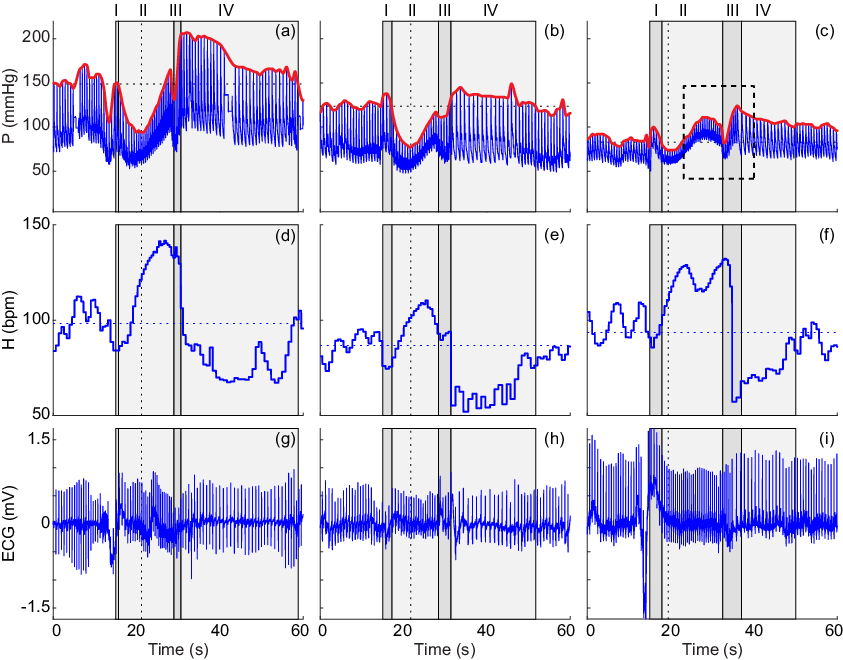
We aim to categorize disease and healthy states based on a two-parameter bifurcation analysis. We show that the sympathetic time-scale, , and sympathetic delay, , parameters are intrinsically linked and interactions between them can cause oscillations and unstable behavior. The use of stability analysis to examine effects of the delay in the baroreflex response has been done in one study by Ottesen [22]. He performed a two-parameter bifurcation analysis and showed that when the time delay is varied over its physiological range, stability switches arise. However, oscillatory modes were not compared to patient data. In this study, we compare the sympathetic outflow and heart rate responses of two control subjects and a patient with AD exhibiting the M response to the VM as categorized by Palamarchuk et al. [23] (Figure 1), determining parameter regimes where instability occurs. The M behavior is hypothesized as overactive sympathetic and parasympathetic activity. In this study, we analytically determine the locations of the different stability regimes by solving and comparing the homogeneous DDE system to numerical simulations of the associated nonhomogeneous system and discuss the effects of the forcing function on the stability. In addition, we connect these results to physiological data exhibiting instability.
2 Materials and methods
This study analyzes a neurological control model of the autonomic nervous response to the VM. Utilizing systolic blood pressure (SBP, mmHg) and thoracic pressure (, mmHg) as inputs, the model predicts heart rate and sympathetic and parasympathetic nervous system responses.
| Subject | Classification | Age | Sex | ||
|---|---|---|---|---|---|
| (years) | (mmHg) | (bpm) | |||
| 1 | Control | 21 | Female | 149 | 98 |
| 2 | Control | 27 | Male | 117 | 87 |
| 3 | POTS with M behavior | 57 | Female | 83 | 94 |
- 1.
POTS - postural orthostatic tachycardia syndrome.
- 2.
- mean systolic blood pressure.
- 3.
- mean heart rate.
2.1 Data
Blood pressure (, mmHg) and electrocardiogram (ECG, mV) measurements were collected via a Finometer (Finapres Medical Systems BV, Amsterdam, The Netherlands) and a precordial ECG-lead, respectively, and saved in LabChart for three subjects performing a Valsalva maneuver. All subjects gave consent to participate in this study and the protocol was approved by the Ethics Committee for the Capital Region, Denmark. Heart rate (, bpm) was computed in LabChart using cyclic detection for human ECG. Table 1 summarizes the data used in this study. The blood pressure, heart rate, and ECG data for all subjects are shown in Figure 1. SBP is calculated as the interpolation of consecutive local maxima in the blood pressure (Figures 1a-c red curve). Subjects 1 and 2 exhibit no AD and Subject 3 has postural orthostatic tachycardia syndrome (POTS), determined as an increase in heart rate of 30 bpm without an associated increase in blood pressure during a postural change [33]. Subject 3 exhibits the M blood pressure response to the VM as categorized by Palamarchuk et al. [23] (Figure 1c dashed black box).
2.2 Valsalva maneuver
The Valsalva maneuver (VM) is a clinical test that involves forced expiration while maintaining an open glottis [11]. In response to a sudden decrease in blood pressure, the VM initiates the baroreflex, which inhibits parasympathetic and stimulates sympathetic activity, increasing heart rate [5].The VM is divided into four phases (illustrated in Figure 1):
- 1.
The breath hold causes a sharp increase in blood pressure and slight decrease in heart rate.
- 2.
Phase II is divided into two sections:
- (a)
Early phase II: Blood pressure drops below baseline significantly, triggering parasympathetic withdrawal and heart rate acceleration.
- (b)
Late phase II: Delayed sympathetic activation accelerates heart rate further and increases peripheral vascular resistance, resulting in an increase in blood pressure.
- (a)
- 3.
Release of the breath hold causes a sharp decrease in blood pressure, triggering a second parasympathetic withdrawal.
- 4.
Increased sympathetic activation causes blood pressure to overshoot and return to baseline within 30 s, while normalization of parasympathetic activity causes a sharp drop in heart rate and subsequent return to baseline.
2.3 Model overview
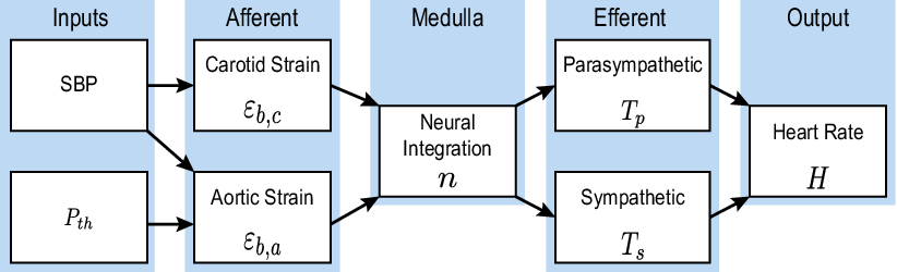
The model analyzed in this study is from our previous work in Randall et al. [24] but does not account for the respiratory sinus arrhythmia (RSA). Since the RSA sub-model does not depend on the effect the sympathetic delay, we remove this model component and focus solely on the baroreflex sub-model. A schematic of the baroreflex model is given in Figure 2.
The open-loop model takes SBP data and as inputs predicting heart rate and parasympathetic and sympathetic responses. For simplicity, the thoracic pressure is modeled as
| (1) |
where and are the start and end of the VM from the data as shown in Figure 3. Due to the delay in sympathetic signal transduction, the model incorporates a discrete time-delay, , into the differential equation modeling sympathetic outflow, giving the following system of equations:
| (2) |
where . The states are the carotid (, dimensionless) and aortic (, dimensionless) baroreceptor strains, the parasympathetic (, dimensionless) and sympathetic (, dimensionless) outflows, and the heart rate (, bpm). (dimensionless) and (s) for , , , or denoting baroreceptor, parasympathetic, sympathetic, and heart rate, respectively, are the gains and time-scales for each of the differential equations with units and values given in Table 3. (bpm) denotes the intrinsic heart rate of 100 bpm, and (dimensionless) and (dimensionless) are gains scaling parasympathetic and sympathetic outflow, respectively. Initial conditions and constant history value are summarized in Table 2. Arterial wall strain for or denoting the carotid sinus and aortic arch, respectively, is a nonlinear sigmoid-like function predicting arterial wall deformation given by
| (3) |
for the carotid () and aortic () pressures, where (mmHg-1) and (mmHg) are the steepness and half-saturation values and (dimensionless) is an offset parameter. The saturation functions for or are the sigmoidal relations
| (4) |
where (s) and (s-1) are the steepness and half-saturation values and
| (5) |
is a convex combination of the relative strains.

In summary, the model consists of 5 differential state equations and 20 parameters with one DDE. The model has the form
| (6) |
where is the right hand side, is the state vector, is the constant history vector, is the discrete delay, and is the parameter vector
| (7) |
where each . Nominal parameter values are summarized in Table 3 and an explanation of parameter assignments is given in the Appendix.
| Symbol | Units | Description | Nominal |
|---|---|---|---|
| value [24] | |||
| Cross-sectional area ratio | 5 | ||
| s | Neural integration parameter | 0.5 | |
| Baroreceptor strain gain | 0.1 | ||
| Baroreflex-parasympathetic gain | 5 | ||
| Baroreflex-sympathetic gain | 5 | ||
| s | Baroreceptor strain time-scale | 0.9 | |
| s | Baroreflex-parasympathetic time-scale | 1.8 | |
| s | Baroreflex-sympathetic time-scale | 10 | |
| s | Heart rate time-scale | 0.5 | |
| mmHg | Arterial wall strain sigmoid steepness | 0.04 | |
| s | Baroreflex-parasympathetic sigmoid steepness | 10 | |
| s | Baroreflex-sympathetic sigmoid steepness | 10 | |
| mmHg | Arterial wall strain half-saturation value | ||
| s | Baroreflex-parasympathetic half-saturation value | 0.55 (A1) | |
| s | Baroreflex-sympathetic half-saturation value | 0.06 (A2) | |
| bpm | Intrinsic heart rate | 100 | |
| Baroreflex-parasympathetic heart rate gain | 0.220.04 (A3) | ||
| Baroreflex-sympathetic heart rate gain | 0.370.2 (A4) | ||
| s | Sympathetic delay parameter | 3 | |
| s | Valsalva maneuver start time | data | |
| s | Valsalva maneuver end time | data |
- 1.
A blank space in the Units column indicates the parameter is dimensionless.
- 2.
A mean one SD is reported where applicable.
- 3.
denotes the baseline systolic blood pressure as listed in Table 1.
- 4.
“data" refers to the fact that this quantity was taken directly from the data.
2.4 Physiological model reduction
To analyze of the effect and dynamics of the DDE, we reduce the model to two states, the baroreflex-mediated sympathetic tone (the DDE) and heart rate , which is affected by the DDE. Since the model is open-loop, the other three states (, , and ) are not impacted by the DDE. To establish the two-state model, we eliminate these states by forming algebraic relations, taking advantage of short time-scales as explained below.
First, since the model is open-loop, there is no feedback to the states that come before the delayed state , i.e., , , and , as shown in Figure 2. For the purposes of this analysis, we assume these states remain in steady-state for the entire time interval, and hence, we can reduce them algebraically. We reformulate the differential equation for as
| (8) |
Since the time-scale is an order of magnitude smaller than , we remove this differential equation by setting and solving for , giving
| (9) |
We make a similar simplification for the baroreceptor strains ( for or ), taking advantage of the small time-scale in relation to the magnitude of . Thus,
| (10) |
Second, since we are interested in the instability caused by the VM, we accentuate the effect of the increased thoracic pressure () during to the VM by eliminating the carotid pathway. With this simplification, the model depends solely on the effect of the aortic baroreceptors, that is, we set and
| (11) |
The resulting model is a system of two states, and , of the form
| (12) |
The reduced system is in the form of equation (6), where , for , is a discrete delay, and is the vector of parameters
| (13) |
The model outputs for the full model (red, equation (2)) and the reduced model (black, equation (12)) in comparison to the heart rate data from Subject 1 are shown in Figure 4.

The model in equation (12) is linear with respect to the states and reformulating the system yields
The forcing functions (s-1) and (bpm s-1) for and , respectively, are given by
| (22) |
and
| (23) |
This is a nonhomogeneous, nonautonomous DDE system. Forcing functions and represent the dynamics induced by the blood pressure responses to the VM. Since the forcing functions use blood pressure data as an input, we ensure smoothness by filtering the data using the movmean command in MATLAB with a window of one second. Then, we fit a degree polynomial to the filtered signal, that is, the coefficients of a polynomial were optimized to fit the filtered signal. Polynomials of orders 10 produced high frequency oscillatory behavior at baseline. We artificially extended the SBP before the curve to ensure the model began in steady-state and after to accentuate the oscillatory behavior of the signal if it arises. Figure shows the original blood pressure data (blue), the moving mean (red), and the fitted polynomial (gray). Figures 5b and c display the forcing functions and , respectively.

In summary, we consider the system
| (24) |
where is the vector of delayed states, and are constant matrices given as
| (25) |
and is the forcing vector given by
| (26) |
3 Stability analysis
The stability of the DDE in equation (24) depends on both the homogeneous solution and the effect of the forcing function. In this section, we analytically explore the homogeneous equation by classifying the roots of the CE, . We numerically categorize the behavior of the nonhomogeneous, nonautonomous system using Algorithm 1 that takes advantage of the gradient of the solution after the VM occurs.
3.1 Homogeneous system
To analyze the stability of equation (24), we first consider the homogeneous equation
| (27) |
which is expanded as
| (28) | ||||||
| (29) |
In this system, the origin is a unique critical point, i.e., if another critical point exists, then from equation (29), we have
| (30) |
From (28), we have
| (31) |
Therefore, the origin is the only critical point of the system in (27).
Since equation (28) solely depends on the delayed state , we assume its solution to be an exponential equation of the form
| (32) |
where is a scaling factor and is the eigenvalue [1, 3, 27]. We make this assumption since the DDE can reduce to an ordinary differential equation (ODE) in steady-state. Hence, we can find an explicit solution to equation (29) as
| (33) |
Therefore, is linearly related to . As , the exponential term vanishes, that is, for large , is proportional to and the stability of depends explicitly on the stability of . Thus, by analyzing , we inherently know the behavior of . By substituting equation (32) into equation (28), we obtain
| (34) |
Trivially, if , then is a solution to equation (34). Considering the portion of equation (34) in parentheses, we obtain the transcendental, nonlinear CE
| (35) |
Note that . Several curves of the CE are plotted in Figure 6 for and sampled from the interval . can have 2 real roots (gray curve), 1 real root (red curve), or infinitely many complex roots. Examples of solutions with complex roots are also plotted in Figure 6, i.e., for , for . When (green curve), the solutions are stable. For (orange curve), a limit cycle emerges about the origin. When (blue curve), solutions are unstable.

The CE (equation (35)) has been analyzed in terms of the Lambert function for [1, 14, 36] that satisfies
| (36) |
for . To obtain a similar formulation as equation (36), we rearrange the characteristic equation as
| (37) |
and multiply both sides by , which gives
| (38) |
This equation is a Lambert function (equation (36)) for , that is,
| (39) |
Combining equations (38) and (39) gives
| (40) |
Note that the Lambert function contains an infinite number of branches for integer with corresponding solutions . Figure shows several solutions to equation (40) for , varied from , and . Since the focus of this study is the analysis of model behavior in relation to patient data, we are concerned with solutions that have the greatest real part, corresponding to the principal branch, [28]. Therefore, we only analyze the solution for the principal branch, that is, (i) for , the solutions corresponding to for vanish faster than the solution corresponding to ; (ii) for , the solutions corresponding to are either purely oscillatory (as in ) or vanish; or (iii) for , the solution corresponding to dominates and diverges faster than all other solutions.
Case 1: Real Roots. We consider the case where the CE ( equation (35)) has real roots, i.e., and . Taking the derivative of and setting it to zero, we obtain,
| (41) |
for minimizer . Therefore, has real roots if and only if the local minimum of is less than or equal to zero, that is, has real roots. Substituting into equation (35) and setting yields
| (42) |
Since , we have and
| (43) |
This is analogous to the principal branch of the Lambert function. Note that is real- and single-valued for arguments greater than or equal to , i.e.,
| (44) |
When equation (43) is an equality, has one real root and solutions to the origin are critically damped, analogous to the harmonic oscillator. Theoretically, we observe a transcritical bifurcation at this line in the -plane (Figure ), where the critical point changes stability. When equation (43) is strictly greater than, there are two real solutions to that produce overdamped behavior. Hence, the solutions that obey the constraint given in equation (43) are stable.
Case 2: Complex Roots. We consider the case where the CE has complex roots, that is, for and . Without loss of generality, we consider . Then,
| (45) |
Since , both the real and imaginary parts of must also equal to . Thus,
| (46) | ||||
| (47) |
Dividing equation (46) by equation (47), yields
| (48) |
Therefore, it is guaranteed that as long as for . Since we are concerned with the principal branch , we set . Hence, for , and the solutions are asymptotically stable and spiral towards the origin.
When , we have from equation (46)
| (49) |
Once again, we set , since we are concerned with the principal branch . Then, and characterizes the division between stable and unstable behavior [1]. Substituting equation (49) into equation (47) yields,
| (50) |
This line is where crosses the imaginary axis, resulting in a limit cycle. Therefore, theoretically we observe a Hopf bifurcation about the origin in the states (Figure 7). As shown in previous studies [1, 14], instability in the principal branch occurs when
| (51) |
In conclusion, we have shown that for the homogeneous system (equation (27)) there exist two lines across which the behavior of the solutions changes: one at where the solutions to the CE change from real to imaginary and one at where the imaginary roots cross the imaginary axis. These lines are shown in Figure 9a. The former results in a transcritical bifurcation, changing the origin (which is the critical point) from a sink to a stable focus, and the latter results in a Hopf bifurcation, producing a limit cycle about the origin, as shown in Figure 7a. We classify each solution as one of the following types with the corresponding color from the contour in Figure 9a:
- 1.
Sink - overdamped (gray): When , has two real solutions .
- 2.
Sink - critically damped (red): When , has one real solution , determining a transcritical bifurcation.
- 3.
Stable focus (green): When , has complex solutions and .
- 4.
Limit cycle (orange): When , has complex solutions (i.e., ) and a limit cycle about the critical point emerges from a Hopf bifurcation.
- 5.
Unstable (blue): When , has complex solutions for and solutions diverge.

3.2 Nonhomogeneous system
The inclusion of the forcing function, , complicates the analysis, and as discussed in Section 1, tools such as DDE-Biftool [8] and knut [30] are not suitable for the nonautonomous, stiff system given in equation (24). As shown in Figure 5, relies on a polynomial fitted to blood pressure data with baseline extended before and after the dynamic behavior. This forcing function creates a set point at a prescribed equilibrium calculated from the baseline SBP () and heart rate (). A disturbance caused by this function, such as the VM, can result in undesirable model behavior and instability. Moreover, the perturbation of this control system may cause persistent instability, that is, instability as a result of a perturbation caused by a forcing function in which oscillatory behavior arises that either remains unstable, oscillates with constant amplitude, or takes a long time to dampen in relation to the stimulus.
In the previous section, we determined regions of the parameter space where the five different behaviors arise for the homogeneous solution. We do not expect these regions to be the same for the nonhomogeneous solutions, especially since forcing functions can stabilize and destabilize systems [29]. However, we do expect analogous regions corresponding to the behaviors given above.
This numerical experiment explores the impact of sudden, transient effects of the forcing function on the stability of the system in equation (24) given a specified parameter range. For this analysis we consider only the effects of the interactions between and . We chose these parameters to investigate based on the analysis of the homogeneous system, which created stability subregions in the parameter space (equations (43) and (50)). We assume changing these parameters will also cause instability in the nonhomogeneous system. The parameter space for and is with a discretized mesh of step-size with all other parameters remaining constant at their nominal values. The model was evaluated iteratively at every point in the mesh. Since the instability is most prominent after the maneuver and during the recovery, we only consider the stability of the signal after the breath hold of the VM was over.
Numerically, we have developed an algorithm to determine the type of solution behavior summarized in Algorithm 1. Of particular note are the thresholds , , and . and are the maximum and minimum thresholds for the slope of the regression line to determine a limit cycle. is the threshold for the value of the line of regression of the amplitudes of consecutive oscillations determining the goodness of fit. These thresholds ensure a limit cycle is obtained.
Solutions for the homogeneous and nonhomogeneous equations were calculated using the stiff, delay differential equation solver RADAR5 [9]. This is a variable-step solver that employs collocation methods to calculate the history of the delayed states. All initial conditions and constant history value (Table 2) were assigned such that the system begins in steady-state.

- 1.
Calculate (Figure 8b). Only consider after the Valsalva maneuver.
- 2.
Determine where crosses the -axis (Figure 8b).
- 3.
Filter out local extrema if the distance between consecutive points is 0.1 s.
- 4.
1: Let and be vectors of the local maxima and minima and .2: for to N do3: if then4: Remove and from and , respectively.5: end if6: end for7: and are the resulting filtered vectors.
- 5.
Determine the vector of amplitudes .
- 6.
Assign solution behavior.
1: if is empty then2: is a sink.3: else if has 1 entry then4: spirals in.5: else7: Calculate the value of the regression line.8: if then9: if then10: is a limit cycle.11: else12: spirals in.13: end if14: else if then15: spirals out.16: else17: spirals in.18: end if19: end if


4 Results and discussion
Stability analysis is important for understanding the kinds of outputs a model can produce. Moreover, bifurcation analysis explores where changes in parameter values impact the system. In this study, we have analyzed a system of nonautonomous, stiff, delay differential equations (DDEs) that can be written as the sum of a homogeneous system (equation (27)) and its associated nonhomogeneous component including the forcing vector given in equation (26). Figure 9 displays the results of the stability analysis with a two-parameter bifurcation diagram plotted for both the homogeneous system (Figure 9a) and the nonhomogeneous system (Figure 9b in equation (12)) denoted with the following colors:
- 1.
Sink - overdamped (gray): The inclusion of the forcing function increases the range of the stable region within the parameter space, that is, the gray region extends beyond the red line in Figure 9b.
- 2.
Sink - critically damped (red): There is a shift in the red line denoting the transcritical bifurcation from the homogeneous contour to the nonhomogeneous contour, as the sink region expands. This relation is no longer a line but a curve between the sink and stable focus regions.
- 3.
Stable focus (green): The stable focus region shrinks with the inclusion of the forcing function, resulting in an oscillatory contour that is steeper than the red line predicted in the homogeneous system.
- 4.
Limit cycle (orange): The limit cycle occurs in the same location in both the homogeneous and the nonhomogeneous bifurcation contours. This is most likely due to the fact that the large amplitude oscillations begin to dominate the signal.
- 5.
Unstable (blue): The unstable region is the same in both the homogeneous and nonhomogeneous contours. This is to be expected as the solutions diverge.
Figure 10 displays representative curves from each region mentioned above for both (Figure 10a and 10b) and (Figure 10c and 10d). For the nonhomogeneous system (Figures 10b and 10d), the solutions begin in steady-state and the forcing function induces the VM, causing some of the responses to have oscillatory behavior. Holding constant at its nominal value, we varied showing that as decreases, we see a shift in the behavior of the model output from sink (gray) to stable focus (green) to limit cycle (orange) to unstable (blue). We observe that though and are within their individual physiological ranges, their interactions cause persistent instability for decreasing values of . Therefore, to ensure that the model produces physiologically relevant results, restricting the parameter space to remain in the sink and stable focus regions is necessary.
Bifurcation packages, e.g., DDE-Biftool [8], cannot be used to conduct the analysis of the nonautonomous, stiff system of delay differential equations discussed here. Moreover, the forcing function is not periodic, so packages, such as knut [26, 30], cannot be utilized to analyze equation (12). Therefore, we developed our own algorithm to qualitatively assess the behavior of the solutions propagated after the implementation of the VM. This algorithm classifies the behavior of the solutions starting after the transient VM stimulus by quantifying consecutive amplitudes. With this algorithm, we were able to effectively categorize the solutions and determine the boundary between the sink and stable focus regions.
| Subject | Classification | Stability region | Color | ||
|---|---|---|---|---|---|
| 1 | Control | 9.2 | 7.5 | Sink | Gray |
| 2 | Control | 4.7 | 5.4 | Stable focus | Green |
| 3 | POTS with M behavior | 5.6 | 5.2 | Stable focus | Green |

Figure 11 shows the heart rate model fits for the reduced two-state model (red, equation (12)) and full five-state model (black, equation (2)) and the resulting trace for each subject: Subject 1 is a control subject exhibiting sink behavior (Figures 11a and d); Subject 2 is a control subject exhibiting stable focus behavior (Figures 11b and e); and Subject 3 has POTS also exhibiting a stable focus behavior (Figures 11c and f). The model was solved for 120 s to extend the signal and allow oscillations sufficient time to dampen. Parameter values and where they fall in the bifurcation diagram (Figure 9) are given in Table 4. As shown in Figure 11, control subjects can have both sink and stable focus behavior. This could be due to the fact that some subjects have naturally higher baseline sympathetic activity or due to undiagnosed autonomic dysfunction.
The M behavior is hypothesized to be the result of overactive sympathetic and parasympathetic activity [23]. Figure 11f demonstrates that the baroreflex control mechanism is very sensitive for this subject, causing oscillatory dynamics that are generally not seen in most control subjects [24]. With the stability analysis, we are able to characterize the dynamics of the M behavior as well as support that the M behavior may be due to instability in the negative feedback control of the baroreflex stimulating a sympathetic response.
When comparing the full and reduced model outputs in Figure 11, we observe that the full model induces more smoothing of the heart rate than the reduced model. The amplitudes of the reduced model are larger than those of the full model. This is to be expected, since the full model has more differential equations with varying time-scales, which can smooth the solutions. Despite this, the reduced model displays a good approximation of the full model. The parameter values used in the both model formulations are given in Table 4. Note that the full and reduced models agree in the type of signal behavior. Hence, the reduced model with its inherent simplicity can successfully detect persistent instability in these subjects.
We do not see limit cycles or unstable modes in practice. This is most likely due to the fact that when one system becomes inordinately overactive, there are many other redundancies in place to reset the body, such as inducing syncope [5]. However, we can classify each of these stability regions not only on the basis of their mathematical properties but of their clinical relevance. These categories are:
- 1.
Sink: Healthy/control behavior within the “normal" range.
- 2.
Stable focus: Potential dysfunction caused by overactive sympathetic behavior.
- 3.
Limit cycle: Unphysiological steady pulsation of sympathetic activity.
- 4.
Unstable: Sympathetic positive feedback that may be unphysiological. (If it is physiological, it may be corrected via other regulatory mechanisms or, in a worst case scenario, cause death).
In this study, we physiologically reduced the full five-state model to a system of two DDEs that can be solved analytically. This simplified both the model and the analysis and proved to be a reasonable reduction of the system (Figure 4). However, numerically, we could have analyzed the full model as opposed to the reduced two-state model. We considered the two-state model for both the homogeneous and nonhomogeneous analyses to facilitate interpretability and comparison.
5 Conclusions
In this study, we analyzed the effect of the delay differential equation system modeling the autonomic response to the Valsalva maneuver and categorized the various types of behavior that can result from the interaction of the delay parameter and the time-scale . Moreover, we classified stability regions both mathematically and physiologically in a two-parameter bifurcation diagram. Motivated by oscillatory behavior that arises in the data, we have determined a numerical relationship between and and observed transcritical and Hopf bifurcations. The model also supports that the M behavior may arise due to oscillatory behavior from overactive sympathetic stimulation.
Appendix
Table 3 lists the nominal parameter values used in the full five-state model. Parameters (dimensionless), (mmHg-1), and (mmHg) are associated with equation (3) and informed by the sigmoid-like relationship given in Mahdi et al. [17]. However, in our formulation, is a half-saturation value defined as the mean systolic blood pressure (, mmHg), which changes for each subject as listed in Table 1. (s-1, equation (5)) varies from 0 to 1, denoting the convex combination of the two afferent signals. We set to model average signaling. Nominal values for the time-scales of the afferent and efferent neural signals were set to literature values: , , and s [15]. bpm [21] is the intrinsic heart rate, i.e., when the heart is completely denervated. The sigmoid steepness parameters for the parasympathetic and sympathetic neural signals ( (s) and (s)) were set to 10 s to account for the order of magnitude of . The sympathetic delay () was assigned a value of 3 s as used in previous modeling studies [15, 34]
Some parameter values were calculated a priori given baseline values ( (mmHg) and (bpm)) from the data. From here on, denotes a steady-state value. Using this notation, the following parameters are calculated as:
| (A1) | ||||
| (A2) | ||||
| (A3) | ||||
| (A4) |
where and are the initial condition and constant history value given in Table 2 and (bpm) is the maximal heart rate as a function of age [31]. Further information on parameter value assignment can be found in Randall et al. [24].
Acknowledgments
We thank Drs. Jesper Mehlsen, Section of Surgical Pathophysiology, Juliane Marie Centre, Rigshospitalet, University of Copenhagen, Denmark, and Louise S. Brinth, Department of Clinical Physiology and Nuclear Medicine, Bispebjerg and Frederiksberg Hospital, Denmark for providing the data analyzed in this study.
Funding
This study was supported by the Division of Mathematical Sciences at the National Science Foundation grant #1246991.
References
- Asl and Ulsoy [2003] Asl, Farshid Maghami and Ulsoy, A Galip. Analysis of a system of linear delay differential equations. J Dyn Syst-T ASME, 125: 215–223, 2003. DOI: 10.1115/1.1568121.
- Banks et al. [2017] Banks, H T; Banks, J E; Bommarco, Riccardo; Laubmeier, A N; Myers, N J; Rundlof, Maj, and Tillman, Kristen. Modeling bumblebee population dynamics with delay differential equations. Ecol Model, 351: 14–23, 2017.
- Bellman and Cooke [1963] Bellman, Richard and Cooke, Kenneth L. Differential-Difference Equations. Elsevier Science, United Kingdom, 1963.
- Bi and Ruan [2013] Bi, Ping and Ruan, Shigui. Bifurcations in delay differential equations and applications to tumor and immune system interaction models. SIAM J Appl Dyn Sys, 12: 1847–1888, 2013.
- Boron and Boulpaep [2017] Boron, Walter F and Boulpaep, Emil L. Medical Physiology: A Cellular and Molecular Approach. Elsevier Inc., third edition, 2017.
- Cheng et al. [2018] Cheng, Lifang; Xiukun, Wei, and Cao, Hongjun. Two-parameter bifurcation analysis of limit cycles of a simplified railway wheelset model. Nonlinear Dyn, 93: 2415–2431, 2018.
- d’Onofrio et al. [2010] d’Onofrio, Alberto; Gatti, Francesca; Cerrai, Paola, and Freschi, Luca. Delay-induced oscillatory dynamics of tumour-immune system interaction. Math Comput Model, 51: 572–591, 2010.
- Engelborghs et al. [2002] Engelborghs, K; Luzyanina, T, and Roose, Dirk. Numerical bifurcation analysis of delay differential equations using DDE-BIFTOOL. ACM Trans Math Solftw, 28: 1–21, 2002. DOI: 10.1145/513001.513002.
- Guglielmi and Hairer [2001] Guglielmi, N and Hairer, E. Implementing Radau IIA methods for stiff delay differential equations. Computing, 67 (1), 2001. DOI: 10.1007/s006070170013.
- Hall [2016] Hall, John E. Guyton and Hall Textbook of Medical Physiology. Elsevier, Inc., Philadelphia, PA, thirteenth edition, 2016.
- Hamilton et al. [1943] Hamilton, W F; WoodBury, R A, and Jr.Harper, H T. Arterial, cerebrospinal, and venous pressures in man during cough and strain. Am Heart J, 27 (6): 871, 1943. DOI: 10.1016/S0002-8703(44)90319-4.
- Keane et al. [2017] Keane, Andrew; Krauskopt, Bernd, and Postlethwaite, Claire M. Climate models with delay differential equations. Chaos, 27: 114309, 2017. DOI: 10.1063/1.5006923.
- Krauskopf and Sieber [2014] Krauskopf, Bernd and Sieber, Jan. Bifurcation analysis of delay-induced resonances of the El Niño Southern Oscillation. Proc Math Phys Eng Sci, 420 (2169): 1–18, 2014.
- Kuang [1993] Kuang, Yang. Delay Differential Equations with Applications in Population Dynamics, volume 191. Academic Press, San Diego, CA, 1993.
- Lu et al. [2001] Lu, K; Clark Jr., J W; Ghorbel, F H; Ware, D L, and Bidani, A. A human cardiopulmonary system model applied to the analysis of the Valsalva maneuver. Am J Physiol Heart Circ Physiol, 281 (6): H2661–H2679, 2001. DOI: 10.1093/cvr/23.8.683.
- Luzyanina et al. [2005] Luzyanina, Tatyana; Roose, Dirk, and Bocharov, Gennady. Numerical bifurcation analysis of immunological models with time delays. J Comp Appl Math, 184: 165–176, 2005.
- Mahdi et al. [2013] Mahdi, Adam; Sturdy, Jacob; Ottesen, Johnny T, and Olufsen, Mette S. Modeling the afferent dynamics of the baroreflex control system. PLoS Comput Biol, 9 (12): 1–18, 2013. DOI: 10.1371/journal.pcbi.1003384.
- Makroglou et al. [2006] Makroglou, Athena; Li, Jiaxu, and Kuang, Yang. Mathematical models and software tools for the glucose-insulin regulatory system and diabetes: an overview. Apl Num Math, 56: 559–573, 2006.
- Nelson and Perelson [2002] Nelson, Patrick and Perelson, Alan S. Mathematical analysis of delay differential equation models of HIV-1 infection. Math Biosci, 179: 73–94, 2002.
- Olsen [2014] Olsen, Christian Haargaard. Modeling Heart Rate Regulation by the Baroreflex. Thesis, North Carolina State University, 2014.
- Olufsen et al. [2005] Olufsen, Mette S; Ottesen, Johnny T; Tran, Hien T; Ellwein, Laura M; Lipsitz, Lewis A, and Novak, Vera. Blood pressure and blood flow variation during postural change from sitting to standing: model development and validation. J Appl Physiol, 99 (4): 1523–1537, 2005. DOI: 10.1152/japplphysiol.00177.2005.
- Ottesen [1997] Ottesen, Johnny T. Modelling of the baroreflex-feedback mechanism with time-delay. J Math Biol, 36 (1): 41–63, 1997. DOI: 10.1007/s002850050089.
- Palamarchuk et al. [2016] Palamarchuk, Iryna S; Baker, Jacquie, and Kimpinski, Kurt. The utility of Valsalva maneuver in the diagnoses of orthostatic disorders. Am J Physiol Regul Integr Comp Physiol, 310 (3): R243–252, 2016. DOI: 10.1152/ajpregu.00290.2015.
- Randall et al. [2019] Randall, Eric Benjamin; Billeschou, Anna; Brinth, Louise S; Mehlsen, Jesper, and Olufsen, Mette S. A model-based analysis of autonomic nervous function in response to the Valsalva maneuver. J Appl Physiol, 2019. DOI: 10.1152/japplphysiol.00015.2019.
- Rao et al. [2018] Rao, Feng; Casillo-Chavez, Carlos, and Kang, Yun. Dynamics of a diffusion reaction prey-predator model with delay in prey: effects of delay and spatial components. J Math Anal Appl, 461: 1177–1214, 2018.
- Roose and Szalai [2007] Roose, Dirk and Szalai, Robert. Continuation and bifurcation analysis of delay differential equations, pages 359–394. Springer, Dordrecht, 2007.
- Ruan and Wei [2003] Ruan, Shigui and Wei, Junjie. On the zeros of transcendental functions with applications to stability of delay differential equations with two delays. Dyn Cont Disc Imp Syst, 10: 863–874, 2003.
- Shinozaki and Mori [2006] Shinozaki, Hiroshi and Mori, Takehiro. Robust stability analysis of linear time-delay systems by Lambert function: some extreme point results. Automatica, 42: 1791–1799, 2006.
- Sipahi et al. [2011] Sipahi, Rifat; Niculescu, Silviu-iulian; Abdallah, Chaouki T; Micheils, Wim, and Gu, Keqin. Stability and stabilization of systems with time delay. IEEE Contr Syst Mag, 31: 38–65, 2011.
- Szalai et al. [2006] Szalai, Robert; Stepan, Gabor, and Hogan, S John. Continuation of bifurcations in periodic delay-differential equations using characteristic matrices. SIAM J Sci Comput, 28 (4): 1301–1317, 2006.
- Tanaka et al. [2001] Tanaka, Hirofumi; Monohan, Kevin D, and Seals, Douglas R. Age-predicted maximal heart rate revisited. J Am Coll Cardiol, 37 (1): 153–156, 2001.
- Vielle and Chauvet [1998] Vielle, Bruno and Chauvet, Gilbert. Delay equation analysis of human respiratory stability. Math Biosci, 152: 105–122, 1998.
- Weimer [2010] Weimer, Louis H. Autonomic testing: common techniques and clinical applications. The Neurologist, 16 (4): 215–222, 2010.
- Wesseling and Settels [1993] Wesseling, K H and Settels, J J. Circulatory model of baro- and cardio-pulmonary reflexes. In Blood Pressure and Heart Rate Variability, volume 4, pages 56–67. IOS Press, Amsterdam, The Netherlands, 1993.
- Wilhelm [2009] Wilhelm, Thomas. The smallest chemical reaction system with bistability. BMC Syst Biol, 9, 2009. DOI: 10.1186/1752-0509-3-90.
- Yi and Ulsoy [2006] Yi, Sun and Ulsoy, A Galip. Solution of a system of linear delay differential equations using the matrix Lambert function. In Proc Am Control Conf, pages 2433–2438. IEEE, 2006. DOI: 10.1109/ACC.2006.1656585.