Phase transition in a 1d driven tracer model
Abstract
The effect of particle overtaking on transport in a narrow channel is studied using a 1d model of a driven tracer in a quiescent bath. In contrast with the well-studied non-driven case, where the tracer’s long-time dynamics changes from sub-diffusive to diffusive whenever overtaking is allowed, the driven tracer is shown to exhibit a phase transition at a finite overtaking rate. The transition separates a phase in which the stationary bath density profile, as seen in the tracer’s frame, is extended, as in the non-overtaking case, to a phase with a localized bath density profile. In the extended phase the tracer velocity vanishes in the thermodynamic limit while it remains finite in the localized phase. The phase diagram of the model as well as the tracer velocity and the bath density profile in both phases are studied, demonstrating their distinct features.
I Introduction
The motion of a tracer (or a tagged particle) in a bath of identical particles confined to a narrow channel is a classical problem which has attracted a wealth of theoretical and experimental attention over the past several decades. For a sufficiently narrow channel, where particles cannot overtake one another, the motion of the tracer is rather constrained due to strong spatial and temporal correlations between particles, which are generated by the geometrical confinement. The resulting dynamics is famously known as single-file diffusion, in which the tracer’s mean-square displacement grows sub-diffusively at long time as , rather than linearly as in ordinary diffusion (jepsen1965dynamics; percus1974anomalous; alexander1978diffusion). One aspect of single-file diffusion is its evident fragility as the channel becomes wide enough to allow particles to overtake one another. Indeed, as numerous studies have demonstrated, as soon as overtaking becomes possible a smooth crossover from single-file to ordinary diffusion occurs with diffusion dominating at asymptotically long times for any finite overtaking rate (sane2010crossover; siems2012non; kumar2015crossover; ahmadi2017diffusion).
New developments in experimental techniques, such as microrehology (wilson2011small) and microfluidics (kirby2010micro), have recently made it possible to control and manipulate interacting particle fluids at the scale of a single particle, usually by employing optical or magnetic means (grier2003revolution; wittbracht2010flow). Such experimental tools have already been used in many studies of complex fluids with constrained dynamics such as polymer solutions (gutsche2008colloids; kruger2009diffusion; wang2016holographic), colloids (polin2008autocalibrated; dullens2011shear) and granular systems (candelier2010journey). On the theoretical side, these advances have raised considerable interest in geometrically constrained systems in which the tracer is driven by an external force, while the bath particles are not (burlatsky1992directed; burlatsky1996motion; de1997dynamics; landim1998driven; benichou1999biased; illien2013active; cividini2016exact; cividini2016correlation; kundu2016exact; benichou2018tracer).
A broadly studied and interesting aspect of such non-equilibrium settings is their stationary behavior. In the absence of overtaking, the mean velocity of a driven tracer on a finite ring of sites is known to scale as , vanishing as (burlatsky1992directed; burlatsky1996motion; de1997dynamics; oshanin2004biased; illien2013active). Moreover, the stationary bath density profile, as seen in the tracer’s reference frame, is macroscopic and extends throughout the entire system. We henceforth refer to a phase with these properties, namely, vanishing of the mean velocity and a macroscopic bath density profile, as the "extended" phase. On the other hand, for sufficiently large overtaking rates the tracer’s motion is clearly unrestricted by the bath particles, implying a finite tracer velocity and a bath density profile which is localized around the tracer. We refer to a phase with these properties as the "localized" phase.
An interesting question is how does the steady state of the driven system change from extended to localized as the overtaking rates are increased. Is it like in the non-driven setting, where the sub-diffusive, single-file behavior crosses over to ordinary diffusion at any overtaking rates, or does the system remain in the extended phase for some finite overtaking rates. In this case the system would exhibit a nonequilibrium phase transition to the localized phase at some finite overtaking rates.
In this paper we address this question by considering a driven tracer model and studying its behavior in the presence of overtaking. Using a combination of mean-field (MF) analysis and direct numerical simulations, we compute the characteristic properties of the model, including the tracer velocity and the stationary bath particle density profile. Our studies show that the model exhibits two distinct stable phases: An extended phase and a localized phase. The extended phase remarkably persists at finite overtaking rates, changing to the localized phase via a continuous nonequilibrium phase transition. This surprising observation stands in contrast with the well-established equilibrium paradigm in which any finite overtaking rate results in a smooth crossover from single-file sub-diffusion to plain diffusion.
The paper is organized as follows: In Section II we introduce the model. The main results are presented in Section III. In Section IV, the MF analysis is presented, demonstrating the existence of two distinct phases, the extended phase and the localized phase. There we explore various properties of these phases and the transition between them. In Section V we describe the numerical procedure used in the numerical analysis. In Section VI concluding remarks are given.
II The Model
We consider a ring of sites labeled by , occupied by one tracer particle and bath particles of average density . The particles interact through simple exclusion, whereby each site holds one particle at most. Bath particles attempt to hop to vacant neighboring right or left sites with equal rates , whereas the tracer is asymmetric, attempting to hop to the right with rate and to the left with rate . To incorporate the possibility of overtaking into our 1d model, the tracer tries to exchange places with a bath particle occupying its neighboring sites to the right with rate and to the left with rate , if a bath particle is present. The dynamics may thus be represented as follows
where vacant sites, bath particles and the tracer are respectively denoted by and and the rates of each process are depicted along the corresponding arrows.
The case of vanishing exchange rates , for which no overtaking takes place, has been extensively studied in the past. Here we are interested in the effect of exchange processes on the properties of the model. To this end we shall work in the tracer’s reference frame, whose position is defined to be the site , and study the bath density profile at sites . It is worthwhile noting that this model exhibits “particle-hole” symmetry, meaning that it is invariant under the simultaneous transformation of bath particles into holes (or vacancies) implying , together with the transformation of hop rates into exchange rates , (as is evident in Eqs. (4) and (5)). This symmetry places bath particles and holes, as well as hop and exchange processes, on equal footing. For example, a tracer hopping into a vacant site (or hole) can equivalently be thought of as the tracer exchanging places with a hole. Although this symmetry is model-specific and not universal, its signature will nevertheless appear in the following section which announces our main results.
III Main Results
The following results, obtained by MF calculations and numerical simulations, demonstrate the existence of both a localized phase and a robust extended phase, which persists in the presence of exchange. A non-equilibrium phase transition separates the extended phase, characterized by a vanishing tracer velocity and an extended bath density profile from the localized phase characterized by a finite tracer velocity and a localized density profile.
The model’s phase diagram is most conveniently presented when the hopping and exchange rates are rewritten as
| (1) |
where and are the average hopping and exchange rates, respectively, while and are the biases, with and . Our MF analysis yields two critical manifolds, at the mean bath densities and , given by
| (2) |
Since the two manifolds are independent of the average rates and , the MF phase diagram may be represented in the 3d parameter space . For convenience, and without loss of generality, we hereafter consider (or ). The MF phase diagram in the plane is depicted in Fig.

1 for the hop bias . A different section, in the plane, is presented in Fig.
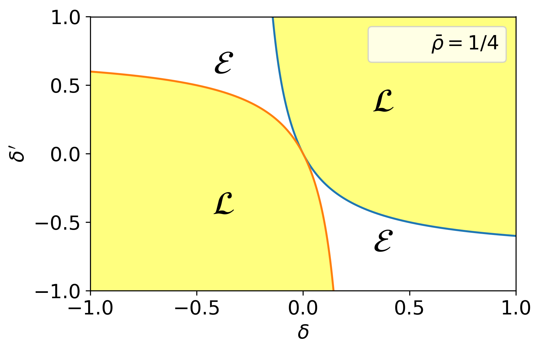
2 for the mean density .
The phase diagram and the nature of the phase transition may be understood as follows: For small and , there are but a few bath particles behind the tracer with which it can exchange places. Consequently, hopping dominates over exchange and a positive stationary tracer velocity arises, characteristic of the localized phase. In this phase the moving tracer generates, in its reference frame, a stationary bath-particle density profile with an induced density excess localized ahead of the tracer. The extent of this region and the number of bath particles entrained in it are of compared with . As increases, more bath particles are found behind the tracer, making the exchange process more pronounced. For a negative exchange bias bath particles are thus effectively "pumped" from behind the tracer, increasing the density excess region ahead. As approaches the critical density , the extent of this region grows and the tracer’s velocity continuously decreases to zero
| (3) |
with the constant given in Eq. (23). At the transition, where , the density excess region ahead of the tracer becomes macroscopic and of , its velocity vanishes and a transition to the extended phase takes place. The continuity of at the transition indicates that the transition itself is continuous.
The following figures provide firm support for this picture, presenting direct simulation results alongside MF calculations. They are generated for the choice of hop and exchange rates , , which conveniently correspond to the rates used in the phase diagram in Fig. 1. For clarity, we shall refer to this particular choice as the "canonical” rates.

In Fig. 3 the tracer velocity is plotted as a function of the mean density for a lattice of size . At low density , the system is in the localized phase with due to the hopping bias . When crosses , the system exhibits a transition to the extended phase in which is vanishingly small. Particle-hole symmetry yields a similar picture as further grows past , leading the system back into the localized phase, this time with due to the exchange bias . The dependence of is illustrated in Fig.

4 in which is plotted versus the inverse system length . It is evident that the velocity in the extended phase vanishes as whereas, in the localized phase appears to decay to a non-zero value for large . In Fig.


5 we present the stationary bath density profile in the tracer’s frame. Panel A shows a data collapse as a function of in the extended phase, where the density excess ahead of the tracer is macroscopic, extending throughout the system. Panels B and C show a collapse as a function of in the localized phase. There, the density excess is localized, leaving the density in the rest of the system effectively unchanged . The excellent agreement in Figs. 3 and 5 between the numerical simulation results and the MF calculations suggests that the model’s stationary behavior is well approximated by the MF description. Figure 6 shows that the change from a macroscopic density profile to a localized one takes place at the phase transition manifolds. Mean field analysis of the density profile at the transition shows that it spans over an intermediate distance that scales as . Namely, that the density profile becomes a function of .

IV Mean Field Analysis
We next compute the stationary properties of the model, focusing on the bath density profile and tracer velocity. To this end, we first formulate rate equations for the bath occupation variable at time and sites in the tracer’s reference frame, where its own position is set to . The occupation variable takes the value if site is occupied by a bath particle at time and otherwise. Let be the average density at site . Applying the MF approximation whereby correlations between site occupations are neglected, i.e. , the evolution equations for are obtained. The equation for in the bulk of the system, i.e. at sites , is given by
| (4) |
whereas, at the first and last sites and , the density satisfies the boundary equations
| (5) |
The tracer’s moving rates to the right and left are given by
| (6) |
The tracer velocity and total moving rate are thus given by
| (7) |
The stationary bulk equation (4) then becomes
| (8) |
where is
| (9) |
The solution of this equation is simply given by
| (10) |
where the parameters , and are determined by the boundary Eqs. (5) and by the normalization requirement
| (11) |
Within this framework, we consider two possible behaviors for the dependence of the tracer velocity , and therefor of , in the limit of large . We will show that depending on the parameters defining the model, the velocity is either in line with the extended phase or as expected in the localized phase.
IV.1 The Extended Phase
Let us first consider the density profile of Eq. (10) with a constant which scales at large as
| (12) |
corresponding to a tracer velocity , as expected in the extended phase. Here is a constant which is yet to be determined. At large , a continuum limit of Eq. (8) is obtained. In this limit the density profile becomes a scaling function of and may be expressed as for the scaling variable , where . The solution of this equation is straightforward and given by
| (13) |
The parameters and are determined by the boundary equation
| (14) |
and the normalization condition , which reduces to
| (15) |
with given by
| (16) |
The densities and can be determined using the boundary Eqs. (5), which also contains the densities and . However, the scaling form of the density profile with implies that and , up to negligible corrections of . As such, and are recovered as
| (17) |
When inserted into Eq. (14) and using the normalization condition of Eq. (15), these expressions give in terms of and provide an explicit (transcendental) equation for ,
| (18) |
It is interesting to observe that the extended phase exists only when the hopping bias and the exchange bias have opposite signs. This simply follows from the normalization property of the density profile for any site and, in particular, . It is also important to note that the density profile , for the particular choice of rates and , has previously been computed using the matrix-product ansatz (derrida2002large). The profile obtained by this method is exact and remarkably coincides with the MF expression derived above. However, for this specific choice of rates, our MF analysis shows that the extended phase persists for any value of the mean bath density , implying that no phase transition takes place for this exactly soluble case.
We conclude that the extended phase is characterized by a vanishing tracer velocity , with determined by a closed transcendental equation which explicitly depends on the rates and on the mean bath density. In addition, we find that the bath density profile becomes a scale function and extends throughout the entire system.
IV.2 The Localized Phase
We next consider the case of for large . Since remains finite at large , the general form of the solution in Eq. (10) implies that the deviation of the bath density profile from the mean bath density must be localized to an region ahead of the tracer. In other words, decays exponentially to with . For , the density profile is then given by Eq. (10) with , such that
| (19) |
Consequently, we find that , up to corrections which decay exponentially with . Using these in the boundary Eq. (5) for , one finds
| (20) |
Collecting these results allows determining through the Eqs. (6), (7) and (9) as
| (21) |
We conclude that the localized phase is characterized by a finite tracer velocity, which explicitly depends on the rates and mean bath density, as well as a localized bath density profile which only deviates from near the tracer.
IV.3 Transition manifolds and critical behavior
Let us consider the localized phase with . To determine the transition manifolds and reported in Eq. (2) we note that in Eq. (21), and so the tracer velocity in the localized phase, vanish at the mean bath density . Moreover, at this average density one can straightforwardly verify (see Eqs. (17), (19), (20)) that and implying that the density profiles in the two phases coincide. Thus, one finds a smooth transition from the localized to the extended phase when the average density reaches . A similar analysis for yields the other transition manifold related to the particle-hole symmetry of the model at an average density .
It is interesting to note that as the transition is approached from the extended phase the parameter (which controls the velocity of the tracer in this phase) diverges. This can be seen by approximating the transcendental Eq. (18) for large to obtain
| (22) |
yielding a divergent at . This divergence signifies the transition from a tracer velocity which scales like , in the extended phase, to the finite velocity expected in the localized phase.
The tracer’s velocity may be considered as the order parameter of the transition. It vanishes in the extended phase and it grows continuously when the transition to the localized phase is crossed. For small deviations from the critical density, i.e. , the velocity of the tracer in the localized phase becomes
| (23) |
In the localized phase the order parameter thus grows linearly with the deviation of the mean density from its critical value .
IV.4 Density Profile at the Transition
In this section we study the bath density profile and the tracer velocity at the critical manifold . A similar analysis can be carried out at the other critical manifold with similar results. We show that on the critical manifold the density profile varies on an intermediate scale of between the microscopic scale of the localized phase and the macroscopic scale characterizing the extended phase. Moreover, on this manifold the tracer’s velocity scales as .
To derive these results we consider the model at density and follow the analysis carries out in the extended phase. Here, though, we take the large- continuum limit
| (24) |
with , and self-consistently deduce the values of and at the transition. With this scaling variables the density profile takes a form similar to that of the extended phase
| (25) |
where and have to be determined by the stationary boundary Eqs. (5) and the normalization condition
| (26) |
For large we take the continuum limit of Eq. (26), for which
| (27) |
such that Eq. (26) yields
| (28) |
up to corrections which decay exponentially with . Using this result in Eq. (25) for , one finds
| (29) |
To determine , we make use of the stationary boundary Eqs. (5) for . Specifically, we take
| (30) |
where denotes the finite-size correction to the asymptotic (i.e. ) density at site (see Eq. (17)). We obtain the -dependence of by substituting of Eq. (29) and of Eq. (30) into the boundary equation for , finding
| (31) |
where
| (32) |
Here we have used the fact that up to higher order corrections.
Having obtained the dependence of , we finally use it in the relation to determine and . To this end recall that , where and are given in Eqs. (6) and (7), depends explicitly on and , providing the relation
| (33) |
to leading order in . Since the only dependence is on the left hand side, we deduce that
| (34) |
and obtain
| (35) |
Combining this result for the velocity with the expressions for the velocity in the extended and localized phases close to criticality, one can write down the scaling form of the velocity in the vicinity of the transition. For a density , with a small perturbation, the velocity scales as
| (36) |
where the scaling function is given by
| (37) |
V Numerical Simulation Procedure
In this section, the simulation procedure which has been used to obtain the numerical results for the model introduced in Sec. II is presented.
Each realization of the dynamics began with drawing the positions of bath particles uniformly over a lattice of sites and then drawing the tracer position uniformly over the remaining sites. Initial tracer hop and exchange times were then drawn from exponential distributions with the respective hop and exchange rates and . For the bath particles, the Gillespie algorithm was used to draw the initial bath hop time from an exponential distribution with rate , accounting for both right and left hops (gillespie2007stochastic). The dynamics was carried out as follows: The smallest of the times and was first determined. If this was , a bath particle was drawn uniformly over the bath particle indices, as well as a random direction . The bath particle would then hop to its neighboring right/left site (in the direction and , respectively) if the site was vacant. If instead one of the tracer hop times, and , was the smallest, the tracer would hop to the right/left neighboring site if that site was vacant. If one of the tracer exchange times, and , was the smallest, the tracer would exchange places with a bath particle to its right/left if a bath particle was present at that site. In case the smallest time was one of the tracer times , the value was added to a counter which followed the position of the tracer with respect to its initial position. For any of the above options, a corresponding new time was drawn and the remaining times were updated.
In Figures 3, 4, 5 and 6 which describe the stationary properties of the system, where the relevant order of limits is , the system was sampled every sweep (consisting of hop attempts, on average) for a total of samples (depending on the value of and ). This number of realization has been chosen such that no noticeable changes were detected at longer times. Each of these figures are the result of averaging different realizations.
VI Conclusions
In conclusion, our study suggests that geometrically-constrained driven tracer transport may exhibit a phase transition from single-file to localized behavior when overtaking processes are allowed. These results are based on a study of a simple lattice gas model in which the extended phase appears when the hopping bias and exchange bias are in opposing directions. This feature is particular to the model in question and may not be required to sustain the extended phase in realistic physical systems. In this context, it would be interesting to explore more realistic and detailed models of transport in geometrically constrained set-ups such as that of hard core particles moving in a narrow channel where the particle overtaking rate is controlled by the width of the channel. Molecular dynamics studies of this model will be considered separately.
The present study is focused on the steady state properties of the model. The phase transition found in this model is also expected to affect the tracer’s dynamical properties, such as the temporal evolution of its mean square displacement. This is left for a future study. Another interesting direction is to study the behavior of multiple tracers in this model. Preliminary studies show that tracers strongly attract each other, generating a macroscopic condensate whose properties are in-line with those predicted in the extended phase. We leave this discussion to a forthcoming publication.
Acknowledgements.
We thank Julien Cividini, Satya Majumdar and Oren Raz for suggestions and critical reading of the manuscript. This work was supported by a research grant from the Center of Scientific Excellence at the Weizmann Institute of Science.References
- (1) DW Jepsen. Dynamics of a simple many-body system of hard rods. Journal of Mathematical Physics, 6(3):405–413, 1965.
- (2) Jerome K Percus. Anomalous self-diffusion for one-dimensional hard cores. Physical Review A, 9(1):557, 1974.
- (3) S Alexander and P Pincus. Diffusion of labeled particles on one-dimensional chains. Physical Review B, 18(4):2011, 1978.
- (4) Jimaan Sané, Johan T Padding, and Ard A Louis. The crossover from single file to fickian diffusion. Faraday discussions, 144:285–299, 2010.
- (5) Ullrich Siems, Christian Kreuter, Artur Erbe, Nadine Schwierz, Surajit Sengupta, Paul Leiderer, and Peter Nielaba. Non-monotonic crossover from single-file to regular diffusion in micro-channels. Scientific reports, 2:1015, 2012.
- (6) AV Anil Kumar. Crossover from normal diffusion to single-file diffusion of particles in a one-dimensional channel: Lj particles in zeolite zsm-22. Molecular Physics, 113(11):1306–1310, 2015.
- (7) Sheida Ahmadi and Richard K Bowles. Diffusion in quasi-one-dimensional channels: A small system n, p, t, transition state theory for hopping times. The Journal of chemical physics, 146(15):154505, 2017.
- (8) Laurence G Wilson and Wilson CK Poon. Small-world rheology: an introduction to probe-based active microrheology. Physical Chemistry Chemical Physics, 13(22):10617–10630, 2011.
- (9) Brian J Kirby. Micro-and nanoscale fluid mechanics: transport in microfluidic devices. Cambridge university press, 2010.
- (10) David G Grier. A revolution in optical manipulation. nature, 424(6950):810, 2003.
- (11) F Wittbracht, A Weddemann, A Auge, and A Hütten. Flow guidance of magnetic particles by dipolar particle interaction. In 2010 Fourth International Conference on Quantum, Nano and Micro Technologies, pages 102–106. IEEE, 2010.
- (12) Christof Gutsche, Friedrich Kremer, Matthias Krüger, Markus Rauscher, Rudolf Weeber, and Jens Harting. Colloids dragged through a polymer solution: Experiment, theory, and simulation. The Journal of chemical physics, 129(8):084902, 2008.
- (13) Matthias Krüger and Markus Rauscher. Diffusion of a sphere in a dilute solution of polymer coils. The Journal of chemical physics, 131(9):094902, 2009.
- (14) Chen Wang, Xiao Zhong, David B Ruffner, Alexandra Stutt, Laura A Philips, Michael D Ward, and David G Grier. Holographic characterization of protein aggregates. Journal of pharmaceutical sciences, 105(3):1074–1085, 2016.
- (15) Marco Polin, Yohai Roichman, and David G Grier. Autocalibrated colloidal interaction measurements with extended optical traps. Physical Review E, 77(5):051401, 2008.
- (16) Roel PA Dullens and Clemens Bechinger. Shear thinning and local melting of colloidal crystals. Physical review letters, 107(13):138301, 2011.
- (17) Raphaël Candelier and Olivier Dauchot. Journey of an intruder through the fluidization and jamming transitions of a dense granular media. Physical Review E, 81(1):011304, 2010.
- (18) SF Burlatsky, GS Oshanin, AV Mogutov, and M Moreau. Directed walk in a one-dimensional lattice gas. Physics Letters A, 166(3-4):230–234, 1992.
- (19) SF Burlatsky, G Oshanin, M Moreau, and WP Reinhardt. Motion of a driven tracer particle in a one-dimensional symmetric lattice gas. Physical Review E, 54(4):3165, 1996.
- (20) J De Coninck, G Oshanin, and M Moreau. Dynamics of a driven probe molecule in a liquid monolayer. EPL (Europhysics Letters), 38(7):527, 1997.
- (21) C Landim, S Olla, and SB Volchan. Driven tracer particle in one dimensional symmetric simple exclusion. Communications in mathematical physics, 192(2):287–307, 1998.
- (22) O Bénichou, AM Cazabat, A Lemarchand, M Moreau, and G Oshanin. Biased diffusion in a one-dimensional adsorbed monolayer. Journal of statistical physics, 97(1-2):351–371, 1999.
- (23) P Illien, O Bénichou, C Mejía-Monasterio, G Oshanin, and R Voituriez. Active transport in dense diffusive single-file systems. Physical review letters, 111(3):038102, 2013.
- (24) Julien Cividini, Anupam Kundu, Satya N Majumdar, and David Mukamel. Exact gap statistics for the random average process on a ring with a tracer. Journal of Physics A: Mathematical and Theoretical, 49(8):085002, 2016.
- (25) J Cividini, A Kundu, Satya N Majumdar, and D Mukamel. Correlation and fluctuation in a random average process on an infinite line with a driven tracer. Journal of Statistical Mechanics: Theory and Experiment, 2016(5):053212, 2016.
- (26) A Kundu and J Cividini. Exact correlations in a single-file system with a driven tracer. EPL (Europhysics Letters), 115(5):54003, 2016.
- (27) O Bénichou, P Illien, G Oshanin, A Sarracino, and R Voituriez. Tracer diffusion in crowded narrow channels. Journal of Physics: Condensed Matter, 30(44):443001, 2018.
- (28) G Oshanin, O Bénichou, SF Burlatsky, and M Moreau. Biased tracer diffusion in hard-core lattice gases: Some notes on the validity of the einstein relation. In Instabilities and Nonequilibrium Structures IX, pages 33–74. Springer, 2004.
- (29) B Derrida, JL Lebowitz, and ER Speer. Large deviation of the density profile in the steady state of the open symmetric simple exclusion process. Journal of statistical physics, 107(3-4):599–634, 2002.
- (30) Daniel T Gillespie. Stochastic simulation of chemical kinetics. Annu. Rev. Phys. Chem., 58:35–55, 2007.