SU(4) Heisenberg model on the honeycomb lattice with exchange-frustrated perturbations: Implications for twistronics and Mott insulators

Let us start with a brief description of the local degrees of freedom of the magnetic species that we are investigating. We assign to each site a spin 1/2 as well as an orbital degree of freedom corresponding to quantum numbers $S^{z}=\pm\frac{1}{2}$ and $\tau^{z}=\pm\frac{1}{2}$, respectively. The Hilbert space of each site $i$ is then spanned by four states $\left|S_{i}^{z},\tau_{i}^{z}\right\rangle$ (often called colors) which are labeled as

The operators for spin ($\mathbf{S}_{i}$) and orbital ($\boldsymbol{\tau}_{i}$) obey the usual SU(2) algebra $\left[S_{i}^{\alpha},S_{j}^{\beta}\right]=i\epsilon^{\alpha\beta\gamma}S_{i}^{\gamma}\delta_{ij}$, $\left[\tau_{i}^{\alpha},\tau_{j}^{\beta}\right]=i\epsilon^{\alpha\beta\gamma}\tau_{i}^{\gamma}\delta_{ij}$ and $\left[S_{i}^{\alpha},\tau_{j}^{\beta}\right]=0$ and are represented by the Pauli matrices in their respective spaces.

The orbital degree of freedom may describe, for instance, a low-energy $e_{g}$ doublet $\left\{d_{3z^{2}-r^{2}},d_{x^{2}-y^{2}}\right\}$ in Mott insulators with octahedral crystal field Khaliullin 2005. Alternatively, it may refer to $p_{x}$ and $p_{y}$ orbitals in optical lattices Wu 2008 or twistronic systems Venderbos and Fernandes 2018. The doublets in these two cases constitute the orthogonal eigenstates of the $\tau^{z}$ operator. We will be concerned only with Hamiltonians that remain invariant under $C_{3}$ rotations around the normal axis of the honeycomb lattice. Similar $C_{3}$ rotations on the internal orbital subspace spanned by $(\tau^{z},\tau^{x})$ accounts for the effect of the spatial transformations on the orbitals. The remaining component $\tau^{y}$ has a distinct role that is more easily seen by the effect of the time-reversal operator $\Theta$. In the orbital space, $\Theta$ reduces to a complex conjugation and leads to $\Theta\boldsymbol{\tau}\Theta^{-1}=\left(\tau^{x},-\tau^{y},\tau^{z}\right)$. The physical interpretation of $\tau^{y}$ is that it distinguishes between states with different orbital chiralities (Yuan and Fu 2018) and is, therefore, related to orbital-magnetic orders Venderbos and Fernandes 2018.

We now introduce the minimal model proposed for the Mott insulating phase of Ba₃CuSb₂O₉ and TBG in Refs. (Smerald and Mila 2014; Venderbos and Fernandes 2018). Despite the different nature of the orbitals in these systems, their in-plane symmetries enable one to assign the same Hubbard model in both cases. The interactions $H_{I}$ are restricted to be onsite:

in which $c_{i,\alpha,s}=c_{\alpha,s}(\mathbf{r}_{i})$ is the annihilation operator of an electron at position $\mathbf{r}_{i}$ on the honeycomb lattice with orbital state $\alpha=1,2$ (corresponding to $\tau^{z}=\pm\frac{1}{2}$, respectively) and spin $s=\uparrow,\downarrow$ (for $S^{z}=\pm\frac{1}{2}$). We also introduce the number operator for a given orbital as $n_{i,\alpha}=\sum_{s}c_{i,\alpha,s}^{\dagger}c_{i,\alpha,s}$ and two parameters for electrostatic interactions: the direct Coulomb repulsion $U>0$ and Hund’s coupling $J_{H}>0$. The tunneling between nearest neighbors on the honeycomb lattice is modeled by the tight-binding Hamiltonian

where $\hat{\mathbf{e}}_{1}=\hat{\mathbf{z}},\,\hat{\mathbf{e}}_{2}=-\frac{1}{2}\hat{\mathbf{z}}+\frac{\sqrt{3}}{2}\hat{\mathbf{x}},\,\hat{\mathbf{e}}_{3}=-\frac{1}{2}\hat{\mathbf{z}}-\frac{\sqrt{3}}{2}\hat{\mathbf{x}}$ are unit vectors in the $zx$ plane, and $i$ runs over the A sublattice, i.e., the triangular Bravais lattice. Here we have set the lattice spacing of the honeycomb lattice to $1$. The matrix $\hat{h}_{\alpha\beta}^{(\gamma)}$ depends on the overlap between the orbitals at positions $\mathbf{r}_{i}$ and $\mathbf{r}_{j}$, connected by a link in the direction $\mathbf{r}_{ij}=\mathbf{r}_{j}-\mathbf{r}_{i}=\frac{1}{\sqrt{3}}\hat{\mathbf{e}}_{\gamma}$. Using an analogy with organic chemistry, we can think of two types of hoppings involving $p$ orbitals that are connected by $\sigma$ or $\pi$ bonds, as indicated in Fig. 2. The matrix $\hat{h}_{\alpha\beta}^{(\gamma)}$ is then parameterized as (Smerald and Mila 2014; Venderbos and Fernandes 2018)

where $t_{\sigma,\pi}\equiv t\pm t^{\prime}$.

The KK model derived within second-order perturbation theory in the regime $t,t^{\prime}\ll U,J_{H}$ reads

Here we defined the dimensionless parameters $\xi=t^{\prime}/t$ and $\eta=J_{H}/U$ and the exchange coupling constants $J_{1}=\frac{J}{1-3\eta}$, $J_{2}=\frac{J}{1-\eta}$, $J_{3}=\frac{J}{1+\eta}$, where $J=t^{2}/U$. As usual in KK models, the spin part of the interaction between the electrons at sites $i$ and $j$ is written in terms of the projectors onto states with total spin $S=0$ and $S=1$:

Notice that the Hamiltonian is invariant under global spin SU(2) rotations. In contrast, the orbital part of the interaction is in general anisotropic and bond dependent, as it involves the operators

where $\mu,\nu\in\{+,-\}$ and $\hat{\mathbf{e}}_{ij}=\hat{\mathbf{e}}_{\gamma}$ for $\mathbf{r}_{ij}\parallel\hat{\mathbf{e}}_{\gamma}$. Explicitly, we can write the Hamiltonian as

Let us first consider the model with $\xi=\eta=0$. In this case, the original two-orbital Hubbard model in Eqs. (2) and (3) is invariant under global SU(4) color transformations. As a result, at this point the KK model reduces to $\mathcal{H}(0,0)=\mathcal{H}_{\text{SU(4)}}-3NJ$, where $N$ is the number of sites of the honeycomb lattice and $\mathcal{H}_{\text{SU(4)}}$ is the SU(4) Heisenberg model given by

Here we introduce the color exchange operators

which can be recognized as the SU(4) generators Corboz et al. 2012. Any local spin-orbital operator that appears in Eq. (5) can be written as a linear combination of $S_{a}^{b}(i)$ operators. In particular, $\mathcal{H}_{\text{SU(4)}}$ is proportional to the sum of color permutation operators $P_{ij}\equiv\sum_{a,b}S_{a}^{b}(i)S_{b}^{a}(j)$ over all nearest-neighbor bonds.

In the case of isotropic hopping ($\xi=0$) but nonzero Hund’s coupling ($\eta>0$), the Hamiltonian is given by

Thus, along the $\xi=0$ line in parameter space, the model retains an SU(2)$\times$U(1) symmetry. The U(1) symmetry is due to the conservation of the orbital chirality, as $\sum_{i}\tau^{y}_{i}$ commutes with the Hamiltonian.

For general values of $\xi$ and $\eta$, model (5) exhibits a global SU(2)$\times\mathbb{Z}_{3}$ symmetry, where the $\mathbb{Z}_{3}$ symmetry is associated with $\pm 120^{\circ}$ orbital rotations about $\tau^{y}$ accompanied by the rotation of the bond directions. The bond-dependent hopping $t^{\prime}$ introduces the exchange-frustrated perturbations given in Eq. (8). Of particular interest are the points $\xi=\pm 1$ with $\eta=0$, where Eq. (5) becomes

The orbital interactions take this form because Eq. (4) involves a projector to either $\sigma$ or $\pi$ bonds (Fig. 2). Hence, the electrons interact with each other only if they both occupy the orbital state which is an eigenstate of $\hat{\mathbf{e}}_{ij}\cdot\boldsymbol{\tau}$ with eigenvalue $\pm 1/2$ for $t^{\prime}=\pm t$, respectively. This type of orbital dependence appears in compass models for $e_{g}$ orbitals Nussinov and van den Brink 2015 or for $j=3/2$ states after projection of $t_{2g}$ states in the limit of strong spin-orbit coupling Natori et al. 2016; Romhányi et al. 2017.

Our choice of ordered states is guided by the symmetries discussed in Subsection II.2. The SU(2) symmetry and the absence of geometric frustration suggest that, classically, the spins form either a ferromagnetic (FM) or an antiferromagnetic (AFM) order. Equation (7) suggests that the orbitals may either align with $\tau^{y}$ or be contained in the $\left(\tau^{z},\tau^{x}\right)$ plane. By computing the classical energy for different orbital configurations, we find that only in-plane orbital-ordered states are competitive. When bond-independent interactions dominate, the system develops ferro-orbital (FOxz) or antiferro-orbital (AFOxz) in the $xz$ plane as illustrated in Figs. 3(b) and (c). On the other hand, interactions proportional to $\left(\hat{\mathbf{e}}_{ij}\cdot\boldsymbol{\tau}_{i}\right)\left(\hat{\mathbf{e}}_{ij}\cdot\boldsymbol{\tau}_{j}\right)$ favor the “vortex” orbital orders displayed in Figs. 3(d) and (e). In fact, the orbital vortex states are the best trial ground states of the compass model on the honeycomb lattice (Wu 2008). They also appear as the exact ground state for a special point of the $JK\Gamma$ model for the honeycomb iridates (Chaloupka and Khaliullin 2015).

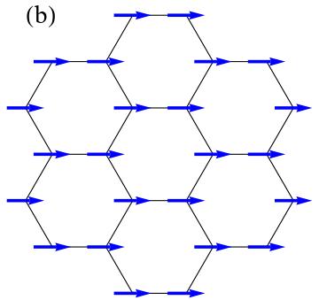
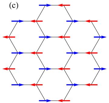
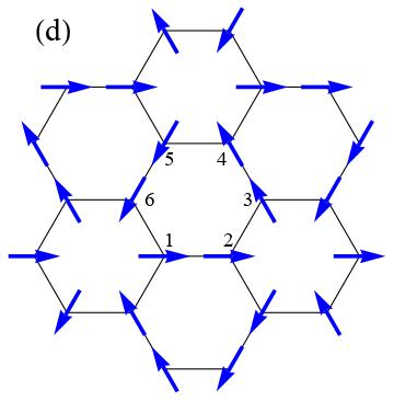
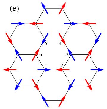
We find that the mean field phase diagram is symmetric under $\xi\mapsto-\xi$. Figure 3(a) shows the phase diagram for $\xi>0$ and $0<\eta<0.3$. In the physically more relevant regime $\xi<1$, we observe a competition between two states with AFOxz order distinguished by the FM or AFM spin order. In agreement with Venderbos and Fernandes 2018, the FM state has lower energy for $\xi\to 0$ at any fixed $\eta$. The transition from AFOxz to the orbital vortex states across the line $\xi=1$ can be attributed to a six-sublattice orbital rotation symmetry of the model discussed in (Smerald and Mila 2014), which maps $\mathcal{H}(\xi,\eta)\mapsto\mathcal{H}(1/\xi,\eta)$ and connects the collinear orbital phases in Figs. 3(b) and (c) to their vortex counterparts in Fig. 3(d) and (e) (Chaloupka and Khaliullin 2015).

A careful analysis of MFT indicates that the classical phase diagram in Fig. 3(a) is incorrect near the point $\xi=\eta=0$, corresponding to $\mathcal{H}_{\text{SU(4)}}$. The reason is that the expectation value $\left\langle\Psi\right.\left|\mathcal{H}_{\text{SU(4)}}\right|\left.\Psi\right\rangle$ is the same for any state in which $\left\langle\psi_{i}|\psi_{j}\right\rangle=0$, i.e., whenever neighboring sites have different colors (Corboz et al. 2012). The number of states satisfying this constraint increases exponentially with the system size and flags the onset of a disordered state. On the other hand, finite Hund’s coupling is expected to favor spin ferromagnetism, in consistency with the FM AFOxz phase. It is then desirable to study the effect of quantum fluctuations on the energy and stability of this spin-orbital ordered state.

LFWT can be viewed as the analog of spin wave theory for spin-orbital models (Joshi et al. 1999). It allows estimates of the excitation dispersion, correction to the zero-point energy and reduction of the order parameter by quantum fluctuations ($\Delta M$) in a single formalism. It also provides some criteria for the stability of a given ordered phase. For example, the application of LFWT to AFM AFOxz leads to dispersion relations with complex frequencies at any $\eta\neq 0$ and $\xi\neq 0$. Such complex dispersion clearly indicates that the AFM AFOxz state is unstable and explains its absence in Fig. 1.

We then study the FM AFOxz state, which is the ordered state with fixed colors $m_{A}=3$ and $m_{B}=1$ on the A and B sublattices, respectively. The Holstein-Primakoff transformation introduces three bosonic species per sublattice labeled by $b_{irm}$, in which $i$ indexes the unit cells, $r$ the sublattices and $m\neq m_{r}$ correspond to the colors in Eq. (1). After replacing spin-orbital operators by their bosonic representations and truncating the Hamiltonian at the level of quadratic terms, the LFWT Hamiltonian is written in the Fourier space as

where $\mathbf{k}$ lies in the Brillouin zone. Here $B_{\mathbf{k}}^{\dagger}$ is a 12-component spinor containing operators of the form

and $\mathcal{H}_{\mathbf{k}}$ is a 12$\times$12 Hermitian matrix. The ordering of the spinor $B_{\mathbf{k}}^{\dagger}$ is motivated by the fact that bosons of colors $m=1$ and $m=3$ are decoupled from bosons with $m=2$ and $m=4$. This implies that $\mathcal{H}_{\mathbf{k}}$ can be written in a block diagonal form as

in which all the block matrices are 4$\times$4. Diagonalization of the LFWT Hamiltonian gives rise to six flavor dispersions $\omega_{\lambda}(\mathbf{k})$ that will be discussed below. We verify that the flavor waves originated from $\mathcal{H}_{\mathbf{k}}^{\left(2,4\right)}$ conserve the total number of bosons, in contrast to what happens for $\mathcal{H}_{\mathbf{k}}^{\left(1,3\right)}$. The constant term in the second and third lines of Eq. (14) gets canceled in the diagonalization and do not contribute to the ground state energy.

Let us now turn to the flavor-wave dispersions $\omega_{\lambda}(\mathbf{k})$ with $\lambda=1,2$, which are related to $\mathcal{H}_{\mathbf{k}}^{\left(1,3\right)}$. Only the exchange constant $J_{1}$ appears in this sector of the LFWT Hamiltonian as a global multiplicative factor. Therefore, the shape of the dispersions $\omega_{\lambda}(\mathbf{k})$ does not vary with $\eta$ and the bandwidth is directly proportional to $J_{1}$. Figure 4(b) shows $\omega_{\lambda}(\mathbf{k})$ for $\xi=0$ in solid lines. In this case, we observe two degenerate bands with linear dispersion at the $\Gamma$ point. This degeneracy is lifted by bond-dependent interactions as shown in Fig. 4(b). The resulting band retains a Goldstone mode and another gapped mode.

We now turn to stability criteria given by $\omega_{\lambda}(\mathbf{k})$ with $\lambda=3,...,6$ obtained from $\mathcal{H}_{\mathbf{k}}^{\left(2,4\right)}$ (see dashed lines in Figs. 4(a) and (b)). First, these bands become zero-energy flat bands in the limit $(\xi,\eta)\rightarrow(0,0)$. This provides another indication of the instability of the ordered state at the SU(4)-symmetric point. Second, $\omega_{\lambda}(\mathbf{k})$ become negative depending on the values of $\eta$ and $t^{\prime}$, which provides yet another instability flag. The region in which this form of instability disrupts an otherwise favored FM AFOxz phase was found numerically and is indicated in gray in Fig. 1. Reference (Smerald and Mila 2014) also encountered an unidentified phase with ED for small clusters in a close region of the parameter space. LFWT suggests that such phase still exists in the thermodynamic limit, but it is incapable of diagnosing its characteristics. When these bosonic modes display strictly positive frequencies, they do not alter the LFWT ground state. Thus, they do not affect the reduction of the order parameter nor the zero-point energy. The energy of the ordered state calculated with LFWT, $E_{\text{LFWT}}$, considers then only the integration of the modes $\lambda=1,2$ and is given by:

The correction to the order parameter is provided by Fig. 4(c), which shows that $\Delta M\sim 0.14-0.25$ when $\xi<0.99$. We observe a divergence of $\Delta M$ as $\xi\rightarrow 1$. This is consistent with the mean-field phase transition occurring at this point due to the six-sublattice mapping discussed above, see Fig. 3. Away from this line, the ordered phase FM AFOxz acquires only mild corrections to the order parameter.

To further check the feasibility of the LFWT energies, we also construct a variational wave function for the ordered FM AFOxz phase, along the line $\xi=0$, following the proposal by Huse and Elser (Huse and Elser 1988). Using standard VMC techniques (Huse and Elser 1988; Ferrari et al. 2017; Gros 1989), we then find the ground state energy as a function of $\eta$, shown in Fig. 4(d). The Huse-Elser energies display a remarkable agreement with the LFWT theory, with only a slightly lower energy. We can then argue that LFWT and variational methods provide consistent results for the FM AFOxz energy, which allows the use of $E_{\text{LFWT}}$ as the estimator for the ordered state energy.

First, we introduce the fermionic parton representation of the SU(4) generators

in which $a=1,...,4$ labels the color states and $i$ labels the lattice site. The fermionic operators satisfy the canonical relation $\{f_{i,a},f_{j,b}^{\dagger}\}=\delta_{ij}\delta_{ab}$ and define a Fock space. Equation (22) is not an exact rewriting of $S_{a}^{b}(i)$ since the physical Hilbert space is isomorphic only to the Fock subspace that satisfies the local single-occupancy constraint $\sum_{a}f^{\dagger}_{i,a}f^{\phantom{\dagger}}_{i,a}=1$. VMC allows an evaluation of averages for observables after implementing a numerical projection to the physical space.

To generate a trial wave function for the QSOL, we first determine the ground state of the mean-field Hamiltonian

where the choice of parameters $\chi_{ij}\in\mathbb{C}$ specify the mean-field ansatz. This ansatz is invariant under SU(4) transformations, thus enforcing a higher symmetry on the state than the SU(2)$\times\mathbb{Z}_{3}$ symmetry of model (5). Translational invariance requires the absolute value of $\chi_{ij}$ to be uniform: $\chi_{ij}=\chi e^{i\phi_{ij}}$, where $\chi>0$ and $\phi_{ij}$ is the phase associated with the link $\langle ij\rangle$. The gauge flux $\Phi$ on each elementary hexagonal plaquette is defined by $e^{i\Phi}\equiv\prod_{\langle ij\rangle\in\hexagon}e^{i\phi_{ij}}$. Here we focus on the $\pi$-flux state with $\Phi=\pi$ through every hexagon Corboz et al. 2012 (see Fig. 5(a)). The corresponding dispersion relation showing a single Dirac cone at the $\Gamma$ point is illustrated in Fig. 5(b).

The ground state at the mean-field level $|\psi_{0}\rangle$ is obtained by filling the lower band shown in Fig. 5(b). We just outline the VMC procedure, since technical details on how to perform the Gutzwiller projection of the mean-field wave functions can be found in the specialized literature (Gros 1989; Corboz et al. 2012; Natori et al. 2016; Natori et al. 2018). The energy of the Gutzwiller-projected $|\psi_{0}\rangle$ is calculated for the KK model in Eq. (8) for different values of $\xi$ and $\eta$ (see Fig. 6). We consider honeycomb lattices of linear length $L$ and $N=2L^{2}$ sites with $L=6$, $12$, and $18$. An initial state for the Monte Carlo evaluation is chosen by randomly placing each color at $N/4$ sites of our lattice. Our Monte Carlo move consists in exchanging a random pair of sites containing distinct colors, which is accepted or rejected according to the general Metropolis algorithm. A Monte Carlo sweep consists of $\sim 10^{3}$ exchanges attempts. After every sweep, we compute the ground state energy $E_{0}$. We typically perform $\sim 10^{5}$ sweeps, with half of the steps discarded for equilibration.

We compared the energy of this particular QSOL to that of the ordered state FM AFOxz. Recall that, as discussed in Sec. III, the AFM AFOxz phase is unstable against quantum fluctuations and disappears completely. We find that the QSOL extends itself away from the SU(4) point, and covers an appreciable portion of the phase diagram before giving room for the FM AFOxz at $\eta\approx 0.175$, a value which is essentially independent of $\xi$. The presence of the FM AFOxz phase at large $\eta$ is expected: Hund’s coupling favors a ferromagnetic spin alignment, while the local Hubbard repulsion favors a staggered orbital occupation (Khomskii 2014). Nevertheless, the QSOL originally identified in Ref. (Corboz et al. 2012) survives the introduction of a finite Hund’s coupling and orbital anisotropy, and it is a competitive ground state for \textcolorblackKK models in the honeycomb lattice.

In Section IV.1, we found that the QSOL is eventually replaced by an ordered state for large enough Hund’s coupling $\eta$. Now we want to investigate different instabilities of the QSOL, specially as a function of $\xi$ and focused on the formation of VBC states. We start this investigation with the tetramerized state. Here the spins form four-site singlet plaquettes breaking translational symmetry but preserving the SU(4) symmetry (Lajkó and Penc 2013). A possible tetramer covering of the honeycomb lattice is illustrated in Fig. 7(a). We tested the stability of the $\pi$-flux state against this tetramerization pattern by considering variational wave functions generated by the mean-field Hamiltonian

Here we keep the $\pi$-flux ansatz, so we modulate the sign of $\tilde{\chi}_{ij}$ as in Fig. 5(d), but we also allow for non-uniform magnitude of the mean-field parameters: $|\tilde{\chi}_{ij}|=\chi^{{\rm tet}}$ if sites $i$ and $j$ belong to the same tetramer and $|\tilde{\chi}_{ij}|=\chi$ otherwise. Furthermore, we define a negative on-site energy $\tilde{\varepsilon}_{i}$ for sites at the center of the tetramers (see sites highlighted in Fig. 7(a)). For $\tilde{\varepsilon}_{i}=0$ and $\chi_{ij}^{{\rm tet}}=\chi$, we recover the uniform $\pi$-flux state. The fully tetramerized state is the product of independent four-site SU(4) singlets throughout the lattice (Li et al. 1998). To quantify the degree of tetramerization of the projected wave functions, we consider the permutation operator between nearest neighbors: $P_{ij}=\sum_{a,b}S_{a}^{b}(i)S_{b}^{a}(j)$, with the color exchange operators $S_{a}^{b}(i)$ defined in Eq. (10). The tetramerization order parameter is defined by (Lajkó and Penc 2013)

where $P_{1}$ is the expectation value of $P_{ij}$ for bonds connecting sites inside a tetramer, while $P_{2}$ is the average of $P_{ij}$ for any other bond (Fig. 7(a)). The parameter $r_{{\rm tet}}\left(\tilde{\varepsilon},\,\tilde{\chi}\right)$ is normalized such that $r_{{\rm tet}}=1$ in the four-site plaquette product state. For each value of $\tilde{\varepsilon}$, we select the value of $\tilde{\chi}=\tilde{\chi}_{{\rm min}}\left(\tilde{\varepsilon}\right)$ that gives the lowest energy within VMC and compute the corresponding tetramerization order parameter $r_{{\rm tet}}\left(\tilde{\varepsilon},\,\tilde{\chi}_{{\rm min}}\left(\tilde{\varepsilon}\right)\right)$. Our VMC results in Fig. 8(a) illustrate that the lowest energy is obtained for $r_{{\rm tet}}=0$ and thus the uniform state is always selected in the region where the QSOL is stable. This implies that the QSOL is stable against tetramerization, in accordance with the results of Ref. (Lajkó and Penc 2013) at the SU(4) point.

Next, we consider valence bond crystals constructed after a mean-field decoupling of spin and orbital degrees of freedom (Smerald and Mila 2014). Since it neglects spin-orbital entanglement, this approximation should break down close to the SU(4) point. Nevertheless, it allows us to search for other trial states which may be stable, for instance, in the region $\xi\sim 1$.

As a first example, we consider that the spins are fully polarized while the orbitals form the collinear dimer pattern shown in Fig. 7(b). A simple product state of orbital dimers produces the following ground state energy: $E_{0}/N=-3(1+\xi^{2})J_{1}$. It is interesting that this energy improves as one moves away from the SU(4) point, in accordance with our general discussion. We also performed a full VMC study with a mean-field Hamiltonian similar to the one in Eq. (24). The dimerization order parameter is $r_{{\rm dim}}=\tilde{P}_{1}-\tilde{P}_{2}$, with $\tilde{P}_{1}$ the average value of the two-color permutation operator on bonds forming a dimer, and $\tilde{P}_{2}$ is the average value for any other bond. By definition, $r_{{\rm dim}}=1$ in the product state discussed previously. Our VMC results in Fig. 8(b) highlight that the lowest energy occurs for $r_{{\rm dim}}=0$ and thus this orbital dimerization is never favored. Moreover, the overall energy is not competitive and this state does not appear in the phase diagram.

Now we assume that the spins dimerize, while the orbitals develop some type of classical order. A spin dimer is clearly not favored by Hund’s coupling and is most likely to be present at small $\eta$. In this limit, a reasonable guess for the orbital dependence would be that orbitals belonging to a spin dimer are parallel. However, ferro-orbital order is too high in energy in the region $t^{\prime}\lesssim t$. Another more promising choice is the ferro-orbital vortex state in Fig. 3(d), coupled to a “Kekule” arrangement of nearest-neighbor spin dimers (Xu et al. 2018). The resulting spin-orbital state is depicted in Fig. 7(c). We follow the nomenclature of Ref. (Smerald and Mila 2014) and refer to it as a noncollinear spin dimers (NCD) phase. To test this state within VMC, we assume ferro-orbital vortex order and perform a VMC calculation in the resulting spin Hamiltonian allowing for spin dimerization, following the same approach as described above. We now find $r_{{\rm dim}}\neq 0$ in the NCD state. Importantly, this is the best variational state in the region $\xi\gtrsim 0.2$ and $\eta\lesssim 0.2$, as indicated by Fig. 6. The detailed comparison of the energies of the variational states FM AFOxz, QSOL, and NCD leads to the phase diagram in Fig. 1. However, we find no competitive candidate, within VMC, for the LFWT unstable region in Fig. 1. In particular, we investigated states with partially polarized spins, following the suggestion of Ref. (Smerald and Mila 2014), but their energy is never competitive (see, for instance, Fig. 8 (b)).

We thank Rafael Fernandes and Johannes Knolle for interesting discussions and critical reading of our manuscript. W.M.H.N. acknowledges the Royal Society for supporting this work through a Newton International Fellowship. This work was supported by the Brazilian agency CNPq (E.C.A.). E.C.A acknowledges the hospitality of the International Institute of Physics (IIP-UFRN), where part of this work was developed. Research at IIP-UFRN is supported by the Brazilian ministries MEC and MCTIC.

References

- Kugel and Khomskii (1982) K. I. Kugel and D. I. Khomskii, Sov. Phys. Usp. 25, 231 (1982).
- Imada et al. (1998) M. Imada, A. Fujimori, and Y. Tokura, Rev. Mod. Phys. 70, 1039 (1998).
- Tokura and Nagaosa (2000) Y. Tokura and N. Nagaosa, Science 288, 462 (2000).
- Khaliullin (2005) G. Khaliullin, Prog. Theor. Phys. Suppl. 160, 155 (2005).
- Krüger et al. (2009) F. Krüger, S. Kumar, J. Zaanen, and J. van den Brink, Phys. Rev. B 79, 054504 (2009).
- Dou et al. (2016) X. Dou, V. N. Kotov, and B. Uchoa, Sci. Rep. 6, 31737 (2016).
- Ueda et al. (2018) H. Ueda, T. Morimoto, and T. Momoi, Phys. Rev. B 98, 045128 (2018).
- Feiner et al. (1997) L. F. Feiner, A. M. Olés, and J. Zaanen, Phys. Rev. Lett. 78, 2799 (1997).
- Nussinov and van den Brink (2015) Z. Nussinov and J. van den Brink, Reviews of Modern Physics 87, 1 (2015).
- Reynaud et al. (2001) F. Reynaud, D. Mertz, F. Celestini, J.-M. Debierre, A. M. Ghorayeb, P. Simon, A. Stepanov, J. Voiron, and C. Delmas, Phys. Rev. Lett. 86, 3638 (2001).
- Mostovoy and Khomskii (2002) M. V. Mostovoy and D. I. Khomskii, Phys. Rev. Lett. 89, 227203 (2002).
- Penc et al. (2003) K. Penc, M. Mambrini, P. Fazekas, and F. Mila, Phys. Rev. B 68, 012408 (2003).
- Vernay et al. (2004) F. Vernay, K. Penc, P. Fazekas, and F. Mila, Phys. Rev. B 70, 014428 (2004).
- Reitsma et al. (2005) A. J. W. Reitsma, L. F. Feiner, and A. M. Oleś, New Journal of Physics 7, 121 (2005).
- Chen et al. (2010) G. Chen, R. Pereira, and L. Balents, Phys. Rev. B 82, 174440 (2010).
- Natori et al. (2016) W. M. H. Natori, E. C. Andrade, E. Miranda, and R. G. Pereira, Phys. Rev. Lett. 117, 017204 (2016).
- Romhányi et al. (2017) J. Romhányi, L. Balents, and G. Jackeli, Phys. Rev. Lett. 118, 217202 (2017).
- Natori et al. (2017) W. M. H. Natori, M. Daghofer, and R. G. Pereira, Phys. Rev. B 96, 125109 (2017).
- Yamada et al. (2018) M. G. Yamada, M. Oshikawa, and G. Jackeli, Phys. Rev. Lett. 121, 097201 (2018).
- Natori et al. (2018) W. M. H. Natori, E. C. Andrade, and R. G. Pereira, Phys. Rev. B 98, 195113 (2018).
- Cao et al. (2018a) Y. Cao, V. Fatemi, S. Fang, K. Watanabe, T. Taniguchi, E. Kaxiras, and P. Jarillo-Herrero, Nature 556, 43 (2018a).
- Cao et al. (2018b) Y. Cao, V. Fatemi, A. Demir, S. Fang, S. L. Tomarken, J. Y. Luo, J. D. Sanchez-Yamagishi, K. Watanabe, T. Taniguchi, E. Kaxiras, R. C. Ashoori, and P. Jarillo-Herrero, Nature 556, 80 (2018b).
- Xu and Balents (2018) C. Xu and L. Balents, Phys. Rev. Lett. 121, 087001 (2018).
- Venderbos and Fernandes (2018) J. W. F. Venderbos and R. M. Fernandes, Phys. Rev. B 98, 245103 (2018).
- Yuan and Fu (2018) N. F. Q. Yuan and L. Fu, Phys. Rev. B 98, 045103 (2018).
- Zhang and Senthil (2019) Y.-H. Zhang and T. Senthil, Phys. Rev. B 99, 205150 (2019).
- Classen et al. (2019) L. Classen, C. Honerkamp, and M. M. Scherer, Phys. Rev. B 99, 195120 (2019).
- Schrade and Fu (2019) C. Schrade and L. Fu, Phys. Rev. B 100, 035413 (2019).
- Wu et al. (2019) X.-C. Wu, A. Keselman, C.-M. Jian, K. A. Pawlak, and C. Xu, Phys. Rev. B 100, 024421 (2019).
- Zhang and Mao (2019) Y.-H. Zhang and D. Mao, arXiv e-prints , arXiv:1906.10132 (2019), arXiv:1906.10132 [cond-mat.str-el] .
- Smerald and Mila (2014) A. Smerald and F. Mila, Phys. Rev. B 90, 094422 (2014).
- Kugel et al. (2015) K. I. Kugel, D. I. Khomskii, A. O. Sboychakov, and S. V. Streltsov, Phys. Rev. B 91, 155125 (2015).
- Affleck and Marston (1988) I. Affleck and J. B. Marston, Phys. Rev. B 37, 3774 (1988).
- Arovas and Auerbach (1988) D. P. Arovas and A. Auerbach, Phys. Rev. B 38, 316 (1988).
- Read and Sachdev (1991) N. Read and S. Sachdev, Phys. Rev. Lett. 66, 1773 (1991).
- Corboz et al. (2012) P. Corboz, M. Lajkó, A. M. Läuchli, K. Penc, and F. Mila, Phys. Rev. X 2, 041013 (2012).
- Nakatsuji et al. (2012) S. Nakatsuji, K. Kuga, K. Kimura, R. Satake, N. Katayama, E. Nishibori, H. Sawa, R. Ishii, M. Hagiwara, F. Bridges, T. U. Ito, W. Higemoto, Y. Karaki, M. Halim, A. A. Nugroho, J. A. Rodriguez-Rivera, M. A. Green, and C. Broholm, Science 336, 559 (2012).
- Nasu and Ishihara (2013) J. Nasu and S. Ishihara, Phys. Rev. B 88, 094408 (2013).
- Huse and Elser (1988) D. A. Huse and V. Elser, Phys. Rev. Lett. 60, 2531 (1988).
- Ferrari et al. (2017) F. Ferrari, S. Bieri, and F. Becca, Phys. Rev. B 96, 104401 (2017).
- Wu (2008) C. Wu, Phys. Rev. Lett. 100, 200406 (2008).
- Joshi et al. (1999) A. Joshi, M. Ma, F. Mila, D. N. Shi, and F. C. Zhang, Phys. Rev. B 60, 6584 (1999).
- Chaloupka and Khaliullin (2015) J. Chaloupka and G. Khaliullin, Phys. Rev. B 92, 024413 (2015).
- Gros (1989) C. Gros, Annals of Physics 189, 53 (1989).
- Savary and Balents (2017) L. Savary and L. Balents, Reports on Progress in Physics 80, 016502 (2017).
- Hermele et al. (2004) M. Hermele, T. Senthil, M. P. A. Fisher, P. A. Lee, N. Nagaosa, and X.-G. Wen, Phys. Rev. B 70, 214437 (2004).
- Khomskii (2014) D. Khomskii, Transition Metal Compounds (Cambridge University Press, 2014).
- Lajkó and Penc (2013) M. Lajkó and K. Penc, Phys. Rev. B 87, 224428 (2013).
- Li et al. (1998) Y. Q. Li, M. Ma, D. N. Shi, and F. C. Zhang, Phys. Rev. Lett. 81, 3527 (1998).
- Xu et al. (2018) X. Y. Xu, K. T. Law, and P. A. Lee, Phys. Rev. B 98, 121406(R) (2018).
- Quilliam et al. (2012) J. A. Quilliam, F. Bert, E. Kermarrec, C. Payen, C. Guillot-Deudon, P. Bonville, C. Baines, H. Luetkens, and P. Mendels, Phys. Rev. Lett. 109, 117203 (2012).
- Katayama et al. (2015) N. Katayama, K. Kimura, Y. Han, J. Nasu, N. Drichko, Y. Nakanishi, M. Halim, Y. Ishiguro, R. Satake, E. Nishibori, M. Yoshizawa, T. Nakano, Y. Nozue, Y. Wakabayashi, S. Ishihara, M. Hagiwara, H. Sawa, and S. Nakatsuji, Proc. Natl. Acad. Sci. 112, 9305 (2015).
- Kang and Vafek (2018) J. Kang and O. Vafek, Phys. Rev. X 8, 031088 (2018).
- Koshino et al. (2018) M. Koshino, N. F. Q. Yuan, T. Koretsune, M. Ochi, K. Kuroki, and L. Fu, Phys. Rev. X 8, 031087 (2018).
- Po et al. (2018) H. C. Po, L. Zou, A. Vishwanath, and T. Senthil, Phys. Rev. X 8, 031089 (2018).
- Seo et al. (2019) K. Seo, V. N. Kotov, and B. Uchoa, Phys. Rev. Lett. 122, 246402 (2019).
- Sharpe et al. (2019) A. L. Sharpe, E. J. Fox, A. W. Barnard, J. Finney, K. Watanabe, T. Taniguchi, M. A. Kastner, and D. Goldhaber-Gordon, arXiv e-prints , arXiv:1901.03520 (2019), arXiv:1901.03520 [cond-mat.mes-hall] .
- Serlin et al. (2019) M. Serlin, C. L. Tschirhart, H. Polshyn, Y. Zhang, J. Zhu, K. Watanabe, T. Taniguchi, L. Balents, and A. F. Young, arXiv e-prints , arXiv:1907.00261 (2019), arXiv:1907.00261 [cond-mat.str-el] .
- Kang and Vafek (2019) J. Kang and O. Vafek, Phys. Rev. Lett. 122, 246401 (2019).
- Kiese et al. (2019) D. Kiese, F. Lasse Buessen, C. Hickey, S. Trebst, and M. M. Scherer, arXiv e-prints , arXiv:1907.09490 (2019), arXiv:1907.09490 [cond-mat.str-el] .
- Ramires and Lado (2018) A. Ramires and J. L. Lado, Phys. Rev. Lett. 121, 146801 (2018).