Approximation Algorithms for Coordinating Ad Campaigns on Social Networks
Abstract
We study a natural model of coordinated social ad campaigns over a social network, based on models of Datta et al. and Aslay et al. Multiple advertisers are willing to pay the host — up to a known budget — per user exposure, whether that exposure is sponsored or organic (i.e., shared by a friend). Campaigns are seeded with sponsored ads to some users, but no network user must be exposed to too many sponsored ads. As a result, while ad campaigns proceed independently over the network, they need to be carefully coordinated with respect to their seed sets.
We study the objective of maximizing the network’s total ad revenue. Our main result is to show that under a broad class of social influence models, the problem can be reduced to maximizing a submodular function subject to two matroid constraints; it can therefore be approximated within a factor essentially in polynomial time. When there is no bound on the individual seed set sizes of advertisers, the constraints correspond only to a single matroid, and the guarantee can be improved to ; in that case, a factor is achieved by a practical greedy algorithm. The approximation algorithm for the matroid-constrained problem is far from practical; however, we show that specifically under the Independent Cascade model, LP rounding and Reverse Reachability techniques can be combined to obtain a approximation algorithm which scales to several tens of thousands of nodes.
Our theoretical results are complemented by experiments evaluating the extent to which the coordination of multiple ad campaigns inhibits the revenue obtained from each individual campaign, as a function of the similarity of the influence networks and the strength of ties in the network. Our experiments suggest that as networks for different advertisers become less similar, the harmful effect of competition decreases. With respect to tie strengths, we show that the most harm is done in an intermediate range.
1 Introduction
Advertising is the most important and successful business model among social network sites. It is widely believed that the adoption of products has a significant social component to it, wherein people recommend products to each other, seek each other’s opinion on products, or simply see others use a product. Under advertising campaigns on social networks, users are shown some ads embedded in their newsfeed from friends; the advertisers’ hope is that the users will voluntarily share the ads, or adopt the product and be observed by their friends using it.
While models and algorithms for viral marketing have a long history of study (e.g., [12, 17, 16, 20, 22], and [8] for a survey), the focus in all of these works (and a much larger body of literature) has been on campaigns to maximize the reach of a single product. When multiple products have been considered, it has typically been in the context of competition, wherein each member of the network adopts at most one product (e.g., [13, 18, 21]); though see [27] for a model wherein products may exhibit complementarities.
Another very important way in which multiple products’ advertising campaigns interact was articulated in two works by Datta, Majumder, and Shrivastava [11] and by Aslay, Lu, Bonchi, Goyal, and Lakshmanan [3]. Both groups of authors observe that marketing campaigns interact in that they involve displaying ads to the same set of users in a social network, and users should not be shown too many ads, lest they feel too inundated with ads and leave the social network [26].11 1 According to the 2012 Digital Advertising Attitudes Report [34], users may even exhibit negative responses towards products if they receive too many advertisements.
More precisely, both sets of authors assume (explicitly or implicitly) that product exposure comes in two forms: sponsored or user-shared. When a user’s friend willingly shares an ad, or the user observes a friend using a product, this is perceived as genuine content. On the other hand, a sponsored ad shown by the network itself is viewed as advertising. Both Datta et al. [11] and Aslay et al. [3] thus impose a constraint on the number of sponsored ads that a user can be shown: the number of sponsored ads shown to node must not exceed a given bound . While only sponsored ads are deemed ‘‘annoying,’’ advertisers do profit equally from sponsored or user-shared exposure. Imposing tight constraints on the number of sponsored ads across ad campaigns, and solving the corresponding optimization problem, should thus reduce the exposure of users to annoying sponsored ads. If the coordinated optimization problem is solved well, then this reduction might be achieved without much reduction in network profit.22 2 Whether users should be shown ads at all on social networks is an ethical and normative question beyond the scope of our work. We take no position on whether social networking platforms should be considered public utilities, financed by subscription fees, or by ad revenue. Our goal here is to limit users’ exposure to sponsored ads while still providing high coverage to individual advertisers in the currently practiced model.
Both Datta et al. and Aslay et al. study the network’s (here also called host) goal of maximizing its own payoff (also called revenue), by carefully coordinating the ad campaigns of multiple advertisers. In both models, the revenue that can be obtained from an advertiser is constrained by the advertiser’s “budget.” In the model of Datta et al., the advertiser pays the host for each user exposure (sponsored or user-shared); however, the number of sponsored ads for advertiser is bounded by some number . In the standard language of influence maximization (precise definitions are given in Section 2), this translates to constraints on the seed set sizes of each advertiser. In contrast, Aslay et al. assume that the advertiser’s budget constrains the total payment for exposures; if an advertiser with budget receives exposures and is willing to pay per exposure, the network’s revenue is .
The advertisers’ hard budget constraints in the model of Aslay et al. raise an interesting question: what happens if , i.e., an advertising cascade reaches more network users than the advertiser is willing to pay for? Aslay et al. [3] posit that the network views this negatively, and incurs a regret over giving the advertiser free exposure.33 3 A possible justification is that if this happens repeatedly, advertisers may learn to lower their declared budget and pay less. In their model, the network obtains regret for undershooting the budget as well, this time over lost potential revenue. Their goal is then to minimize the total regret. Because the regret is 0 only when the network exactly hits the advertisers’ budgets, a straightforward reduction from Partition style problems shows not only NP-hardness, but also hardness of any multiplicative approximation. Under the same model, Tang and Yuan [31] consider a modified payoff function instead of minimizing regret. Their objective function consists of the net revenue generated (capped by the budget), with an additional negative term for excess exposure; this term penalizes overshooting. Notice that over- or undershooting the budget by a small amount in this model does not have as severe consequences for approximation guarantees as it does for the regret objective. As a result, Tang and Yuan achieve a -approximation using a greedy approach.
In this article, like Tang and Yuan, we depart from the regret objective of Aslay et al. In particular, we do not believe that a network incurs ‘‘regret’’ from accidentally giving advertisers free exposure.44 4 Such regret may well be a psychological reality for humans, but it appears less applicable at the level of a major company. One justification for a negative term for overshooting is that advertisers may learn to underbid, waiting for the free higher exposure. However, an equally strong case could be made that giving advertisers free exposure is beneficial, in that it makes the advertisers more likely to run future ad campaigns on the site, which in turn may lead to an increase, not decrease, in future revenue. Once a regret for overshooting the advertiser’s budget is not a concern any more, a much more natural objective is to maximize the network’s total revenue, which is the objective function we study here. (A precise definition of the model is given in Section 2.)
Our main result — in Section 3 — is a general treatment of optimization in this model, subsuming both versions of budgets. We consider very general influence models (potentially different for each advertiser), and only require that the local influence function at every node for every individual advertiser be monotone submodular55 5 Recall that a set function is submodular iff whenever .. Under these assumptions, we show that the network’s revenue can be approximated to within constant factors. More specifically, when there are no constraints on individual advertisers’ seed set sizes (only budget constraints limiting the total number of exposures the advertiser is willing to pay for), then there is a polynomial-time -approximation algorithm, and a simple greedy algorithm achieves a -approximation. When in addition, there are constraints on the seed set sizes of individual advertisers, we obtain a approximation, for every .
We show these results by expressing the optimization problem as a monotone submodular maximization problem over suitably chosen matroid domains, much in the style of Vondrák et al.’s result on welfare-maximizing partitions [6, 35]. As observed by Tang and Yuan as well, when there are no constraints on individual seed set sizes, the constraints jointly define a matroid. This allows us to bring to bear on the problem Vondrák’s polynomial-time -approximation algorithm for maximizing a submodular function subject to a matroid constraint [6, 35] (see also subsequent work [7, 29, 36]), and the much simpler -approximation algorithm due to Fischer et al. [14] (see also [25]). When there are additional constraints on individual seed set sizes, we show that the feasible ad campaigns can be expressed as the intersection of two matroids, and the algorithm of Lee et al. [24] gives a approximation.
While we do not develop new algorithms or heuristics in this part of our work, we consider it an important contribution to explicitly reduce from advertiser competition constraints to the intersections of matroids. Such a characterization was missing from prior work, resulting in heuristics with weaker guarantees and rederiving known arguments. Our work builds on the work of Tang and Yuan and generalizes it to provide a clean optimization framework that allows the incorporation of different constraints in the future, and the application of known powerful optimization techniques and guarantees.
While Vondrák’s beautiful -approximation algorithm for maximizing a submodular function under a matroid constraint [35] runs in polynomial time, it is not practical.66 6 The running time is roughly , with large constants. To the best of our knowledge, the full algorithm has never been implemented, but we would be surprised if it scaled to more than 10 nodes. With this concern in mind, in Section 4, we develop a -approximation algorithm which scales to moderately sized networks comprising several tens of thousands of nodes. Unlike our main results, this algorithm is not fully general, providing guarantees only for the Independent Cascade (IC) Model, and satisfying the budget constraint only in expectation, rather than for each solution. Networks of tens of thousands of nodes are of practical interest: they are often encountered in area-aware advertising [2, 1]. Another natural domain with small networks is targeted health and social intervention programs [38], where network sizes are often only in the hundreds or thousands; it is very plausible that a principal may want to coordinate multiple interventions, such as safe drug usage, safe sex practices, and others.
The reason that the algorithm only works for the IC model is that it is based on randomly sampling Reverse Reachable (RR) sets [4, 32, 33]. These RR sets are then used to define and solve a generalized Maximum Coverage LP, which is then rounded using techniques of Gandhi et al. [15]. An additional important benefit of the algorithm is that the fractional LP which it rounds provides an upper bound on the performance of the optimum solution. This upper bound is useful in our experimental evaluation, not only of the LP rounding algorithm, but of other algorithms as well.
In Section 5, we describe experiments to evaluate the effects of competition and tie strengths on coordinated advertising campaigns. A comparison of algorithms shows that while the greedy algorithm has a worse worst-case approximation guarantee than LP rounding, it performs (marginally) better in experiments; both algorithms beat several natural heuristics, and get within 85% of the LP-based upper bound on the optimum; this is significantly better than their worst-case guarantees. We also develop a parallel version of the Greedy algorithm that accelerates overall processing by a factor of 12 on a 36-core machine. This allows us to scale to graphs with millions of nodes and dozens of advertisers.
Since approximation algorithms for “standard” Influence Maximization have been extensively studied in the literature, our main interest in the experimental evaluation is the effect of competition between products, and the interaction between competition and tie strengths in the network. Our experiments show that the more similar the advertisers’ influence networks, the more the host’s payoff decreases compared to the sum of what could be extracted from the advertisers in isolation. This effect is exacerbated when the network has a small number of highly influential nodes, since each advertiser will only be able to target few of these nodes. When nodes’ influence is more even across the network, the host loses less revenue, because there are enough different “parts” of the network to extract revenue from all advertisers. When ties are very weak or very strong, the effect of competition is again attenuated, while for intermediate tie strengths, competition can lead to a significant revenue loss compared to treating each advertiser separately.
2 Problem Statement
There are advertisers aiming to advertise on a network of nodes/individuals . We will use and (and their variants) to denote nodes, and (and variants) exclusively for advertisers.
Product information (or ads or influence) propagates through the social network according to the general threshold model [22, 28], defined as follows: For each node and advertiser , there is a monotone and submodular local influence function with . Each node independently chooses thresholds uniformly at random for each product . Let be the set of nodes that have shared ad by round . (We call such nodes active for ad .) Node becomes active for ad in round iff . The (random) process is seeded with seed sets (subject to constraints discussed below). It quiesces when no new activations occur in a single round. At that point, for each ad , a final (random) set has become active. The general threshold model subsumes most standard models of influence spread, including the Independent Cascade and Linear Threshold models. Notice that (1) the diffusions for different proceed independently, except for joint constraints on the seed sets (discussed below), and (2) different ads can in principle follow different diffusion models.
Each advertiser has a non-negative and monotone value function giving the payment that will make to the network site as a function of the active nodes in the end. In full generality, this function could depend on the (random) set of nodes that are active for in the end; in this case, we will assume that is also submodular. In most cases, however, all nodes in the network will have the same value to advertiser , in which case will only depend on the cardinality . In this case, we will assume that is (weakly) concave; notice that this is a special case of the previous one, because viewed as a function of (rather than ), the function is submodular. For notational convenience, and in keeping with much of the prior literature, we write for the (random) number of nodes that are active in the end when the process starts with the node set .
A particularly natural case — closest to the definition of Aslay et al. [3] — is when . Here, is the advertiser’s budget, while is the amount he is willing to pay per exposure.
The network’s goal is to choose seed sets for all advertisers , subject to additional constraints discussed below, so as to maximize one of the following two global revenue functions:
| (1) | ||||
| (2) |
Notice the subtle difference between the two definitions: captures the expected revenue from advertisers who are charged for each campaign individually, according to their functions . The objective extends straightforwardly to the case where depends not only on the cardinality of , but on the specific set. In contrast, corresponds to the case in which advertisers are charged according to the expected exposure. An essentially equivalent way of expressing the same objective (up to random noise) is that the revenue is based on the average exposure for advertiser over a large number of campaigns.
Specifically in the context of the linear revenue function with a cap of the budget , this means that under , advertiser is never charged more than for any individual campaign, while under , advertiser ’s budget is not exceeded on average over multiple campaigns.
The main constraint, common to both the models of Aslay et al. and Datta et al., is that each node can be exposed to only a limited number of sponsored ads. We interpret this as saying that for node , there is an upper bound on the number of seed sets it can be contained in, i.e., .77 7 This model in fact subsumes one in which each sponsored ad exposure only activates with some probability : add a new ad node with activation function , and set . Then set , so only the new “ad nodes” can be targeted.
In addition to the node exposure constraints , following the model of Datta et al., we also allow for constraints on the seed set sizes of each advertiser: for each advertiser , the number of seed nodes cannot exceed . In addition, we can constrain the total number of sponsored ads (more tightly): . In summary, our target optimization problem is the following:
Definition 1 (Multi-Product Influence Maximization)
For each advertiser , choose a seed set with , such that .
Subject to these constraints, maximize or .
The Multi-Product Influence Maximization problem is clearly NP-hard, as it subsumes the standard influence maximization problem.
3 A General Result
We begin with a very general treatment. Under the assumptions we make (the are submodular functions of , or concave functions of ), the overall objective functions and are both submodular. In the case of , this is because a non-negative linear combination of submodular functions (in particular: a convex combination of submodular functions) is submodular. In the case of , the reason is that is a monotone submodular function of , and applying a monotone concave function preserves submodularity. In both cases, we can therefore apply the result of Mossel and Roch [28], which guarantees submodularity of the objective for each advertiser, as a function of the seed set.
To deal with the constraints on node exposures and seed set sizes, we use a technique discussed in [6, 35] in the context of finding welfare-maximizing assignments of items to individuals, and also implicit in the work of Tang and Yuan for coordinating multiple advertisers [31]. We create a disjoint union of separate networks (each with the original nodes) for each advertiser , and then consider joint constraints on seed sets that can be selected across all of the separate networks. The overall new network has nodes, one node for each combination of an original node and advertiser . Let denote the set of new nodes for advertiser , the set of new nodes corresponding to the node , an and . The influence function for node is , and thus only depends on the nodes in the network for advertiser . Writing for the (random) final set of active nodes in , the objective function is , which is submodular by construction.
Targeting the node in corresponds to exposing node to ad in the original problem. In this way, the problem is simply to choose a subset . The correspondence between seed sets of and ad seeding choices in the original problem is that . The constraints on the selection of are then that , (as well as ).
Because the sets form a disjoint partition of , the restriction that at most nodes from may be selected defines a partition matroid.88 8 Readers unfamiliar with the standard definitions of matroids and (truncated) partition matroids are directed to Appendix A.1 or [30]. Similarly, because the sets form a partition, the constraint that at most nodes from may be selected defines a different partition matroid. The constraint on the total number of selected nodes can be added to either of these partition matroids, and turns it into a truncated partition matroid. The fact that the exposure constraints and an overall constraint on the total number of seeds together define the independent sets of a matroid, was also proven by Tang and Yuan [31] (Lemma 3). Thus, a consequence of this reduction to the optimization problem on is that the constraints on form the intersection of two matroids: a partition matroid on the sets , and a truncated partition matroid defined by the sets and the overall constraint of on the seed set size. The optimization goal is to select a set , subject to these two matroid constraints, so as to maximize a non-negative, monotone, submodular function. The latter is a well-studied problem. The key results for our purposes are the following:
Theorem 2 (Theorem 3.1 of [24])
There is a simple local search algorithm for maximizing a non-negative non-decreasing submodular function subject to matroid constraints. For any , the algorithm (with suitable termination condition) provides a polynomial-time -approximation.
Theorem 3 ([14])
The greedy algorithm, which always adds the next element maximizing the increase in the objective function (subject to not violating the matroid constraint), is a approximation algorithm for maximizing a non-negative non-decreasing submodular function subject to matroid constraints.
Datta et al. prove an approximation guarantee of for a greedy hill climbing algorithm; as discussed above, they do not consider budget constraints on the total number of exposures. Furthermore, they consider only the special case when all advertisers have the same influence functions at all nodes. Their proof shows that the constraints form a -system for (a generalization of the intersection of two matroids); they then invoke an analysis of Calinescu et al. [6] for such systems. The same result can be obtained by appealing to Theorem 3 instead. By making the connection to the intersection of matroids explicit99 9 Datta et al. also discuss matroids, though mostly to remark that the constraints do not form a matroid, and thus to motivate an analysis in terms of -systems. and invoking Theorem 2 instead, we improve the approximation guarantee for this problem to essentially , under a much more general problem setting.1010 10 It should be noted that the analysis of Datta et al. is not really specific to the model they formulate, and could easily be extended to the general problem statement from Section 2.
As opposed to the model of Datta et al., the model of Aslay et al. does not impose constraints on the seed set sizes of individual advertisers; it only restricts exposure per node and the overall seed set size. As discussed above, these constraints together form a single truncated partition matroid (as opposed to the intersection of two matroids). Thus, as observed by Tang and Yuan, the greedy algorithm guarantees a -approximation for the revenue maximization problem (without a penalty for overshooting), simply by invoking Theorem 3 (Lemma 4 in [31]).
In fact, in this simplified model without advertiser-specific seed set constraints, the approximation guarantee can be improved to by appealing to the following theorem of Vondrák et al.
Unfortunately, while the continuous-greedy algorithm runs in polynomial time, it is not practical.
The main message of this section is that, when focusing on the arguably more natural objective of maximizing the network’s revenue (rather than minimizing regret), non-trivial (and in some cases well-established) algorithmic techniques can be leveraged to obtain algorithms with approximation guarantees essentially matching those of standard influence maximization. These guarantees apply in a wide variety of influence models (allowing for completely different influence functions for different advertisers), and under a variety of constraints about the seed sets for different advertisers. In fact, by leveraging subsequent work on submodular maximization under multiple Knapsack and matroid constraints (see, e.g., [7, 29, 24, 36]), one can also obtain (somewhat weaker) approximation guarantees when different seed nodes have different costs (in terms of money or effort) for targeting.
4 An LP-rounding Algorithm for the Independent Cascade Model
In this section, we focus on the special case of the Independent Cascade (IC) Model for influence in a network, and a budgeted linear valuation function: the payoff the host receives from advertiser is . The IC Model for influence has been widely studied; a reader wishing to briefly review the definition may find a description in Appendix A.2. In talking about the model, we use to denote the probability that an edge activates node for product when node has become active for product .
We use the idea of Reverse Reachability sets [4, 32, 33] to reduce the multi-advertiser campaign coordination problem to a generalized Maximum Coverage problem; we then show how to round the LP, using an algorithm of Gandhi et al. [15], to obtain a polynomial-time and reasonably practical -approximation algorithm for the problem with both node and advertiser constraints.
This approximation guarantee gives an improvement over the -approximation guarantee of the local search algorithm (Theorem 2). When the seed set sizes of individual advertisers are not restricted, the continuous greedy algorithm of Theorem 4 matches the LP rounding algorithm’s guarantee, but the continuous greedy algorithm is completely impractical. The LP rounding algorithm is less efficient than the simple greedy algorithm from Theorem 3, but provides better approximation guarantees.
The downside, compared to the more general treatment in Section 3, is that the results only hold for the IC Model, and the budget constraints on the number of exposures will only be satisfied in expectation: in any one run, the algorithm may charge an advertiser (significantly) more than .
4.1 The Reverse Reachability Technique
A very useful alternative view of the Independent Cascade Model was first shown in [22], and heavily used in subsequent work: generate graphs by including each edge in independently with probability . Then, the distribution of nodes activated by ad in the end, when starting from the set , is the same as the distribution of nodes reachable from in the random graph .
This alternative view forms the basis of the Reverse Reachability Set Technique, first proposed and analyzed by Borgs, Brautbar, Chayes, and Lucier [4], and further refined by Tang, Xiao, and Shi [32, 33]. The primary goal of [4, 32, 33] was to permit a more efficient evaluation of the objective . Under both the Independent Cascade and Linear Threshold Models, evaluating is known to be #P-complete [10, 37]. Reverse Reachability sets permit a more efficient (both theoretically and practically) approximate evaluation, as compared to the obvious Monte Carlo simulation.
We explain the Reverse Reachability technique for a single ad, and omit the index for readability for now. The key insight is the following: let be an arbitrary node, and consider the (random) set of all nodes that can reach in the randomly generated graph . Then, the probability that is activated starting from is equal to the probability that . (See, e.g., [33, Lemma 2].)
More generally, if we draw such sets independently, and for independently uniformly random target nodes , and intersects of them, then is an unbiased estimator of the expected number of nodes activated when starting from . In order to leverage this insight for computational savings in computing ad campaigns, it is important that the estimate be sufficiently accurate with sufficiently high probability, for a small enough number of reverse reachable sets. A characterization of this accuracy is given by the following lemma from [33] (restated slightly here):
Lemma 5 (Lemma 3 of [33])
Assume that
| (3) |
Consider any set of at most nodes. With probability at least , the following inequality holds for :
| (4) |
Here OPT is the maximum influence spread that can be achieved by any set of at most nodes.
Lemma 5 implies that when is large enough to allow taking a union bound over all relevant sets , the fraction of sets that intersect a candidate seed set is an accurate stand-in for the actual objective function . As already observed by Borgs et al. [4], this reduces the problem of influence maximization to a Maximum Coverage problem: selecting a set of at most seed nodes that jointly maximize the number of sets containing at least one seed node.
Without loss of generality, assume that for all . Let be the maximum influence that advertiser could achieve with seed nodes, and ignoring the budget constraint . A lower bound on each can be found by running the TIM algorithm [33] with seed sets of size . For each advertiser , we draw nodes1111 11 This value of is chosen with foresight to apply Lemma 5 and allow the application of various bounds in the following paragraphs. i.i.d. uniformly (in particular, with replacement) from , and for each such , we let be the random reverse reachable set. For later ease of notation, we index the nodes as , and the corresponding sets as . Notice that the same node might appear as for different , with possibly different sets . For each such index of a node and set , let be the unique advertiser such that , and write for the set of all sets used to estimate the influences for advertiser .
Focus on any advertiser , and the influence of any set with . Using Lemma 5 with and , the influence of is estimated to within an additive term with probability at least . By a union bound over all such sets (of which there are1212 12 When running a greedy algorithm, only such sets need to be considered, which leads to significant computational savings. Here, our goal is to leverage the reverse reachability technique not necessarily for significant computational savings, but for improved approximation guarantees. ) and all advertisers , the influence of all such sets is simultaneously estimated to within an additive term of , with probability at least . Assume for the rest of this section that the high-probability event has happened.
Now consider an arbitrary seed set with , not necessarily contained in just one partition . Let , and let be the estimated expected influence of . By the preceding paragraph, the influence of each is estimated to within an additive , i.e., . We next want to show that for each , the actual payoff the host obtains from advertiser , i.e., is estimated to within an additive term ; then, by summing over all advertisers , the total estimation error is at most .
To prove the estimation error bound for an advertiser , we consider several cases. First, if , then the payoff 0 is estimated completely accurately. Second, if , i.e., the advertiser’s budget is so low that he pays for at most one impression, the payoff is also estimated completely accurately. The reason is that for any , all nodes in will always be shown impressions, so with probability 1. As a result, the payoff from the advertiser is estimated correctly as . Finally, if , then . The reason is that the optimum does at least as well as using seed nodes for advertiser , which would yield payoff , because . Thus, the estimation error for the payoff from advertiser is at most .1313 13 Some of the complications in the proof arose because of the possibility of very different budgets and payoffs per node across advertisers. When the payoff per node for all advertisers is equal, i.e., for all , then RR set samples are enough to provide accurate payoff estimates with sufficiently high probability.
4.2 The LP and Rounding Algorithm
Notice that except for the budget caps , the objective is a sum of (scaled) coverage functions. This suggests the natural formulation of an LP, which allows us to use a randomized rounding technique due to Gandhi et al. [15].
Recall that each set is generated by a reverse (random) BFS from a randomly sampled node , where the same node may be sampled for multiple . Also recall that is the unique advertiser for the reverse reachable set , and that is the set of all reverse reachability sets with . We use the decision variable to denote whether node was targeted for ad , for the decision variable whether at least one node from the set was selected (for its corresponding ad), and the variable for the total revenue from advertiser . The optimization objective can be expressed using the following Integer Linear Program (ILP):
| (5) |
The first constraint states that a target node is only covered if at least one node from the set is selected, and the second constraint ensures that the LP derives no benefit from double-covering nodes. The third constraint encodes the bound on the number of targeted ads that can be exposed to, while the fourth constraint encodes the bound on the seed set sizes of the advertisers . The fifth constraint captures the overall bound on the total number of targeted ads. The sixth and seventh constraints characterize the objective function for advertiser .
Of course, solving the ILP is NP-hard, so as usual, we consider the fractional LP relaxation obtained by omitting the final integrality constraint . Without this constraint, the LP can be solved in polynomial time, obtaining a fractional solution .
To round the fractional solution, we use the dependent rounding algorithm of Gandhi et al. (See Section 2 of [15].) This algorithm can be applied to round fractional solutions whenever the variables to be rounded (here: the ) can be considered as edges in a bipartite graph, and constraints correspond to bounds on the (fractional) degrees of the nodes of the bipartite graph.1414 14 The fifth constraint of our LP (overall budget) does not fit in this framework, since it is a constraint on all variables. We extend the rounding algorithm of Gandhi et al. by one more final loop (see below) which repeatedly picks any two fractional variables and randomly rounds them using the same approach as the rest of the algorithm, until only one fractional variable remains. This last variable can then be rounded randomly by itself. It repeatedly rounds the fractional values associated with a subset of edges forming a maximal path or a cycle, until all variables are integral; let denote the rounded (integral) values corresponding to . The algorithm of [15] provides the following guarantees:
- •
The probability that the variable is rounded to is exactly , for all and .
- •
In the bipartite graph, each node’s degree is rounded up or down to an adjacent integer. In the context of our LP (5), this means that the number of seed nodes for each advertiser is either rounded up or down to the nearest integer, as is the number of exposures to sponsored ads for each node. In particular, the third and fourth constraints are satisfied with probability 1.
- •
For any node of the bipartite graph and any subset of incident edges, the rounded values are negatively correlated. In the context of our LP (5), for any advertiser and reverse reachable set , the algorithm guarantees that .
After rounding all the to , for each , we set if at least one has , and for each , we set . Together with the guarantees of Gandhi et al., this ensures that all ILP constraints except possibly the seventh (budget) constraint are satisfied; the budget constraint is discussed more in Section 4.4.
Theorem 6
Under the IC model, with constraints on node exposures and advertiser seed set sizes, the (modified) Gandhi et al. correlated LP-rounding based algorithm is a polynomial-time -approximation algorithm, if advertisers pay based on their expected exposure.
Consider any set . With explanations of some steps given below, the probability that is
The inequality labeled (1) used the negative dependence discussed above. The inequality labeled (2) used the standard bound that for all . The inequality labeled (3) uses that the function is concave, and hence on the interval is lower-bounded by the straight line which agrees with it at the endpoints and , which is the function . Finally, the inequality labeled (4) uses that by the first and second LP constraints. Using the definition of , we now get that
4.3 No Seed Set Size Restrictions
In the model of Aslay et al., and in our experiments in Section 5, there are no restrictions placed on the seed set sizes of individual advertisers; that is, the fourth set of constraints in the LP (5) is missing. In the absence of these constraints, the correlated LP-rounding algorithm of Gandhi et al. [15] can be further sped up. Note that except for the fifth (sum of seed set sizes) constraint, the constraints are a collection of disjoint stars. As a result, the general correlated rounding algorithm of Gandhi et al. can be replaced with their algorithm for stars. The resulting algorithm runs in linear time and is very simple to implement. It first uses the correlated rounding on pairs of variables , corresponding to the same node (and different advertisers) until no such pairs remain; subsequently, as for the general algorithm, we add one more while loop to round pairs of the remaining (which now necessarily correspond to distinct nodes ).
Because there is at most one fractional variable remaining incident on any node or , the second property of the Gandhi et al. rounding algorithm is preserved. The negative correlation property holds inductively, because at most two values are rounded in each step.
4.4 The Budget Constraints
In Theorem 6, we emphasized that advertiser payments have to be based on the expected exposure, rather than the actual exposure. Indeed, using the LP rounding approach, maintaining the budget constraints in each run is not possible without a huge () loss in the approximation guarantee. The reason is that LP (5) has an integrality gap of when the budgets are constrained. Consider the following input: the influence graph is a star with leaves, in which the center node has probability 1 of influencing all its neighbors, and no one else can influence any other node. Thus, any advertiser who gets to advertise to the center node will reach the entire graph.
Suppose that each advertiser has a budget of , and the center node has a constraint of . A fractional solution can allocate a fraction of of the center node to each advertiser; each advertiser then reaches nodes, not exceeding his budget, and the host obtains a payoff of . But any integral solution can only allocate to one advertiser, who will then pay at most his budget . Thus, any integral solution obtains payoff at most .
This problem disappears if each advertiser’s budget must only be met in expectation. In other words, on any given day, the advertiser’s budget could be exceeded, even by a lot. But on average, the advertiser does not pay more for impressions than per day. Because the number of impressions resulting from a particular rounding choice is a random variable in , standard tail bounds (e.g., Hoeffding Bounds) show that the total payment is with high probability close to the expected payment after about days.
5 Experiments
In this section, we describe an empirical evaluation of the relationship between the total revenue to the host and the algorithm used, the number of advertisers, and the total number of sponsored ads. More importantly, we also consider the interplay of competition with the influence strengths in the network and the similarity/dissimilarity of the advertisers’ influence networks. We conducted our experiments on a 36-core Linux server with an Intel Xeon E5-2695 v4 processor at 2.1GHz and 1TB memory. We develop a parallel version of the Greedy algorithm that scales to networks of millions of nodes and tens of millions of edges, with dozens of advertisers (see Section 5.5).
All of our experiments are based on the Independent Cascade (IC) Model. We employed the Reverse Reachability technique to (approximately) compute the influence of node sets more efficiently. In Section 4, we obtained an upper bound on the number of RR sets to guarantee good approximations with high probability. This bound is quite large, and using the corresponding number of sets would not permit us to scale experiments to large networks. We conducted extensive experiments on the number of RR sets that are sufficient to guarantee high accuracy in practice. These experiments are described in detail in Appendix B; the upshot is that RR sets are sufficient to guarantee an estimation error . Therefore, for the experiments reported in the remainder of this section, we used a value of .
5.1 Data Sets and Generation of IC Instances
We used the following four real-world networks, whose key statistics are summarized in Table 1. (Two larger networks used for scalability experiments are described in Section 5.5.)
- •
Facebook [23] is an ego network of a user in Facebook, excluding the ego node.
- •
Advogato [23] is a social network whose nodes are users of the Advogato platform; directed edges are trust links.
- •
DBLP [23] is a citation network in which nodes are papers, and there is a directed edge from to if cites .
- •
NetHEPT [9] is a collaboration network generated from co-authorships in high-energy physics publications.
| Dataset | #nodes | #edges | Type |
|---|---|---|---|
| 2,889 | 2,981 | Undirected | |
| Advogato | 6,542 | 51,127 | Directed |
| DBLP | 12,592 | 49,743 | Directed |
| NetHEPT | 15,229 | 31,376 | Undirected |
In creating influence networks (with edge probabilities ), for most of our experiments, we wanted to avoid the assumption of uniform probabilities on edges commonly made when evaluating algorithms for influence maximization. The reason is that one key aspect of our work is the notion of coordination/competition between different advertisers. When all edges have uniform probabilities , the value of a node is solely determined by its network position. We therefore define a way of generating edge probabilities non-uniformly that gives some nodes intrinsically more importance. For each node , we draw a parameter independently and uniformly from for Facebook, DBLP and NetHEPT, and for Advogato. (The different intervals were chosen to counteract the effects of varying edge densities in the datasets.) We then define . We will discuss below how the are correlated for different .
For all experiments, we set the constraint on the number of sponsored ads that can be shown to node to , i.e., each node can be shown a sponsored ad from at most one advertiser. This results in maximal inter-advertiser constraints for the seed sets. We also performed experiments varying the value of . The outcome of these experiments is that what matters is mostly the ratio . As grows (with fixed), the optimization problem gradually decouples across advertisers. As a result, the most interesting and novel aspects of the model manifest themselves when .
For simplicity, we set each advertiser’s payoff per exposure to . The overall numbers of sponsored ads are varied for different experiments, and discussed below. In our experiments, we did not consider individual advertiser seed set constraints ; such constraints are heavily studied in traditional Influence Maximization experiments, and we wanted to focus on the novel aspects arising due to advertiser competition.
5.2 Comparison between the Algorithms
Our first set of experiments simply compared the performance of our algorithms and several baseline heuristics. We implemented the following algorithms:
- •
Greedy is the standard greedy algorithm for maximizing a submodular function subject to a matroid constraint (Theorem 3).
- •
LP-Rounding is described in Section 4.2.
- •
Max-Degree considers nodes by non-increasing degrees, and assigns them to advertisers in a round-robin order. Each node is assigned to consecutive advertisers.
- •
Eigen-Centrality considers nodes by non-increasing eigenvector centrality1515 15 The eigenvector entries of the leading eigenvector of the graph’s adjacency matrix., and assigns them to advertisers in a round-robin order, as with Max-Degree .
- •
is the value of the optimal fractional solution of the LP (5). It provides an upper bound on the value of the optimal solution, and thus gives us a benchmark to compare the algorithms’ performance to, on an absolute scale.
5.2.1 Varying the total number of seeds
In the first set of experiments, we kept the number of advertisers constant at , and varied the total number of seed nodes. Thus, these experiments are similar to evaluations of standard Influence Maximization algorithms. To avoid strong effects of competition between advertisers (which we are evaluating in later sections), we generated the (and hence the ) independently for each .

Figure 1 shows a comparison of the total host payoff achieved by the algorithms as is varied from to . Both LP-Rounding and Greedy perform significantly better than Max-Degree or Eigen-Centrality. This is not surprising, as the heuristics only consider the network structure, but not the influence probabilities associated with edges. However, the random generation of edge probabilities still ensures that nodes of high degree or high centrality tend to be more influential; hence, in some scenarios (especially with small ), the payoffs of the Max-Degree and Eigen-Centrality heuristics are comparable to those of Greedy and LP-Rounding.
A comparison to the fractional LP solution value shows that both Greedy and LP-Rounding achieve more than 85% of the optimal payoff, which is significantly more than the respective guarantees of and . Experimentally, on these instances, Greedy performed marginally better than LP-Rounding.
5.2.2 Varying the number of advertisers
For the second set of experiments, we varied the number of advertisers from 1 to 20, scaling the number of seeds as , to keep an average of 10 seeds per advertiser. Again, we did not add constraints on the budgets or the individual advertisers’ seed sets.
Using this set of experiments, we also studied the effect (on payoff) of competition between advertisers, as caused by the constraint that each node can only be chosen as a seed for one advertiser.1616 16 If there were no constraint on the number of sponsored ads per node, there would be no competition, and the total payoff would increase linearly in . Note also that the total influence of the seed sets of all advertisers is different from the influence of their seed sets’ union if assigned to one advertiser: while no two advertisers can choose the same seed node, if the different seed nodes influence the same nodes later, they will both derive utility (and the host revenue) from those exposures. Therefore, we made the influence probabilities the same for all , i.e., the same nodes are most influential for all advertisers.
Figure 2 shows the per-advertiser payoff achieved as is varied from 1 to 20. A comparison of the algorithms’ performance yields results similar to those reported in Section 5.2.1. For a single advertiser, the performance of the Max-Degree heuristic is comparable to LP-Rounding and Greedy. As explained earlier, this observation can be attributed to the random generation of uniform edge probabilities. For larger values of , there is a significant difference in the performances of the Greedy and LP-Rounding algorithms vs. the Max-Degree and Eigen-Centrality heuristics. A likely explanation is the following: when many advertisers compete on the same network, Greedy and LP-Rounding can alleviate competition for a limited pool of highly influential nodes by indirectly influencing such nodes using other carefully chosen seeds. In contrast, Max-Degree and Eigen-Centrality do not consider such potential propagation for seed selection.

Another observation is that as a result of the competition, per-advertiser payoff decreases and hence, the total host payoff does not scale linearly in . For a single advertiser, DBLP and Advogato have significantly higher payoff than Facebook and NetHEPT. With 20 advertisers, on the DBLP and Facebook networks, the average payoff per advertiser decreases by factors of 2.8 and 2.4, respectively, while the decrease for Advogato is a factor of 2. Comparatively, NetHEPT exhibits only modest competition, and its per-advertiser payoff decreases only by a factor of . A possible cause for the higher decreases may be the very skewed degree distributions of the DBLP and Facebook networks, which results in a smaller number of extremely valuable nodes, and the fact that Advogato and DBLP are directed, resulting in less symmetry between nodes. The strong competition for DBLP and Facebook can also be observed in the fact that the gradient of the per-advertiser payoff is very negative for small values of . For larger , the decrease becomes less pronounced, because there are many marginally useful seed nodes to choose from.
5.3 Effects of Competition
Next, we focused in detail on the effects of competition on total host payoff. More specifically, the question we were interested in is the following: how does the similarity or dissimilarity of influence networks for different advertisers affect revenue? If the influence networks are very similar, then high-value seed nodes for one advertiser will typically also be high-value for others, and the constraint that no node must be chosen by more than a given number of advertisers (in our experiments: ) will constrain the reach of seed sets. On the other hand, if the influence networks are very different, then different advertisers might focus on different parts of the network, and the host could potentially derive significantly higher payoff.
Since the purpose of these experiments is not to compare the performance of algorithms, but to draw qualitative insights, we ran these experiments only using the Greedy algorithm, which had performed best in our earlier experiments.
For these experiments, we fixed the number of advertisers to and total seeds to . To cover a spectrum of different similarities between networks, we used the following generative model. All advertisers initially have the same edge probabilities . We can assume for simplicity that the graph is complete, by setting whenever is not an edge. A parameter will capture the similarity between the networks for different advertisers. Each advertiser ’s influence strengths are generated independently as follows. Starting from , perform node swaps of the following form: select two vertices independently and uniformly at random, and switch all their associated influence probabilities, i.e., set and for all , and and .
The effect is that the influence networks for all advertisers are exactly isomorphic to each other, i.e., no advertiser has an a priori better network. However, the larger the value of , the more independent the networks are, which we expected to lead to more potential to derive payoff from all advertisers simultaneously.

Figure 3 shows the payoff as a function of . First, notice that the host’s payoff does indeed increase steeply in , nearly linearly for a non-trivial segment. This shows that competition between advertisers for high-impact nodes indeed restricts the host’s payoff; as the advertisers’ influence networks become more dissimilar, the host can extract more payoff from the joint ad campaigns.
Next, we observe that the relative increase in payoff (comparing no swaps vs. swaps) is noticeably higher in the Facebook (a factor of 2.4) and DBLP (a factor of 2.7) networks, compared to the Advogato (a factor of 1.8) and NetHEPT (a factor of 1.3) networks. This aligns with our earlier observations: the Facebook and DBLP data sets seem to have fewer high-influence nodes, as compared to the more even influence of nodes in Advogato and NetHEPT. Thus, ensuring more independence among the isomorphic copies of the Facebook and DBLP graphs creates more potential for additional payoff.
Further, the payoff saturates around just swaps for NetHEPT, as opposed to around swaps for Facebook, Advogato and DBLP. This is likely because networks with more competition require more swaps to completely realize the potential of essentially independent campaigns.
5.4 Effect of Influence Probabilities
For our final set of experiments, we were interested in the interplay between competition and edge strengths. We expected two counter-acting effects: as the probabilities on edges increase, more different seed nodes may become capable of reaching the same large part of the network, thus reducing the negative effects of competition. On the other hand, as the edge probabilities decrease, most cascades will not spread beyond a few nodes; as a result, all parts of the network may provide small influence, so again, the additional detrimental effects of competition could be reduced.
For advertisers, we chose a combined seed set size of , and gave each advertiser a budget of . Different from the earlier experiments, we assigned uniform probabilities of to the edges, and varied the value of . Again, because our goal was to study the interplay between competition and parameters of the model (rather than comparing algorithms), we only used the Greedy algorithm. We were interested in the host’s payoff increase as the number of advertisers is increased from 1 to 20. We call the ratio between the two quantities the relative payoff at , and denote it by .
Figure 4 shows the relative payoff as a function of . The two counter-acting effects produce — for all four networks — a local minimum in . As grows large, the ratio saturates at 20; this is not surprising, as with high enough probabilities, essentially any node will reach the entire graph, and there is in effect no competition, resulting in a 20-fold increase in host payoff.
For Advogato and NetHEPT (the two graphs which earlier showed less susceptibility to competition), the ratio is minimized at the same . However, the underlying reasons appear to be different. Advogato has a high edge density; as a result, advertisements spread to a large portion of the graph even for small ; in particular, already for , the reach of every ad campaign matches the budget . The curve for NetHEPT looks similar, but for different reasons. Here, the reason appears to be that NetHEPT is sparse and exhibits little competition from the start, which is confirmed by the fact that never drops below 15. Here, the advertisers’ budgets are only fully extracted around , but the decentralized nature of the graph ensures lack of harmful competition much earlier, which is why saturates around .
For Facebook and DBLP, the two graphs exhibiting more competition, the minimum is attained at . Notice that the minimum value of for these data sets is significantly smaller and the saturation of happens later than for the other networks. This behavior again shows the stronger competition. Specifically for DBLP, even at , the network only extracted about half of the sum of all advertiser budgets.
5.5 Scalability and Parallelization
We evaluated the scalability of the Greedy algorithm on the following two large datasets:
- •
Pokec [23] is a friendship network from the Slovakian social network Pokec, containing 1,632,803 individuals (nodes), and 30,622,564 directed edges (directed friendships).
- •
Flixster [23] is a social network of a movie rating site where people with similar cinematic taste can connect with each other. It contains 2,523,386 individuals and 7,918,801 (undirected) edges.
We evaluated scalability by measuring the runtime as a function of the number of advertisers . The LP Rounding algorithm does not scale to such large datasets; its limit is a few tens of thousands of nodes and edges.
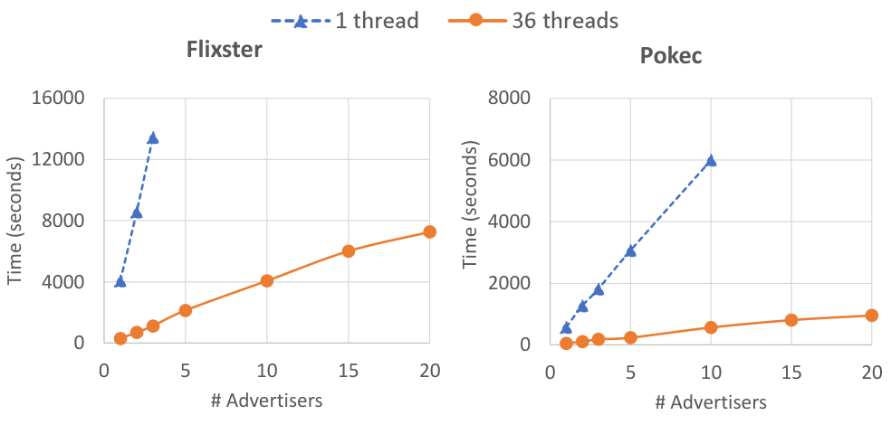
In order to utilize all 36 cores on the server, we parallelized the RR set construction in the Greedy algorithm, which contributes most to the overall execution time. Figure 5 shows that the parallel algorithm can compute seed sets on the large graphs in scenarios with large numbers of competing advertisers, even when the sequential algorithm fails to terminate in a reasonable amount of time. The parallel Greedy algorithm accelerates RR-set construction by a factor about 22 on average, and is overall about 12 times faster than the sequential version.
Due to the large graph sizes and extremely skewed degree distributions in Pokec and Flixster, the highly influential nodes had significantly more impact, and the overall payoff was up to two orders of magnitude larger than for the Facebook, Advogato, NetHEPT and DBLP networks. This resulted in slower seed set selection, which became a significant factor when the RR-set construction was parallelized. As a result, we see that the runtime of our parallel implementation (especially in Pokec) scales sub-linearly with respect to when there are more than a dozen advertisers.
6 Conclusions and Future Work
We explored the problem of maximizing the host’s payoff for a budgeted multi-advertiser setting with constraints on the ad exposure of each node and each advertiser’s seed set size. We showed that under a very general class of influence models, this problem can be cast as maximizing a submodular function subject to two matroid constraints. It can therefore be approximated to within essentially a factor using an algorithm due to Lee et al. [24]; this improves on the -approximation guarantee of [11]. When there are no constraints on individual advertisers’ seed set sizes, only on the total number of seeds, the constraints form just a single truncated partition matroid. Therefore, the algorithm of Vondrák et al. [6, 35] gives -approximation algorithm, while a simple greedy algorithm [14] achieves a -approximation, as observed by Tang and Yuan [31]. For the special case of the Independent Cascade model, the Reverse Reachability Technique [4, 32, 33] can be combined with a linear program and rounding due to [5, 15] to yield a more efficient -approximation algorithm, even under both types of constraints.
Our experiments show that in practice, the greedy algorithm slightly outperforms the LP-rounding based algorithm, despite its worse approximation guarantee. They also reveal that competition between advertisers leads to a loss in payoff for the host when the advertisers’ influence networks are more similar, and particularly so when the networks have few highly influential nodes — in that case, these nodes cannot simultaneously be used as seeds for all advertisers, and the average exposure per advertiser becomes significantly lower than the individual exposures of the advertisers on isolated networks.
Our work was in part motivated by considering a more “natural” objective function than the notion of regret from [3]. As discussed in Section 1, a less Draconian way to penalize excess exposure is to linearly penalize over-exposure. In fact, Tang and Yuan [31] analyze exactly such an objective, simply subtracting the excess exposure from the revenue. They provide a -approximation algorithm for this objective. Their objective function can be further generalized by scaling this penalty term by a user-controlled constant. This allows a host to trade off between the two very different parts of the objective (revenue vs. free exposure), since they are not directly comparable. In additional work not included here, we show that even under this more general model, modifications of the greedy algorithm and LP rounding algorithm still yield constant-factor approximation guarantees.
There are several natural directions for future work. Perhaps most directly, the LP-rounding based algorithm only satisfies the budget constraint in expectation; indeed, we have shown a large integrality gap for the LP. It is a natural question whether a -approximation guarantee can be obtained while always satisfying the budget constraints, and without invoking the heavy Continuous Greedy machinery discussed in Section 3.
We believe that the efficiency, scalability and solution quality of our algorithms, especially the LP-Rounding algorithm (Section 4.2), can be further improved, e.g., by adapting techniques such as the ensemble approach for single-product influence maximization recently proposed by Güney [19]. This method uses multiple batches of a small number of RR sets to generate several candidate seed sets. The key idea here is that the probability of finding an optimal seed increases exponentially in the number of batches, even though smaller RR sets increase the variability of individual candidate sets.
An interesting empirical study would be to evaluate to what extent influential nodes in one advertiser’s network are also influential in other advertisers’ networks. Within typical social networks, one would expect significant differences based on individuals’ expertise; on the other hand, the use of celebrities to endorse products entirely outside their realm of expertise shows that humans appear willing to project expertise in one area on other areas as well.
Acknowledgments
We would like to thank Ajitesh Srivastava for helpful technical discussions. David Kempe was supported in part by NSF Grant 1619458 and ARO MURI grant 72924-NS-MUR.
References
- [1] Helping local businesses reach more customers. https://www.facebook.com/business/news/facebook-local-awareness, 2014.
- [2] Hyperlocal advertising. https://www.wordstream.com/blog/ws/2018/01/25/hyperlocal-marketing, 2018.
- [3] Cigdem Aslay, Wei Lu, Francesco Bonchi, Amit Goyal, and Laks VS Lakshmanan. Viral marketing meets social advertising: Ad allocation with minimum regret. Proc. VLDB Endowment, 8(7):814–825, 2015.
- [4] Christian Borgs, Michael Brautbar, Jennifer Chayes, and Brendan Lucier. Maximizing social influence in nearly optimal time. In Proc. 25th ACM-SIAM Symp. on Discrete Algorithms, pages 946–957, 2014.
- [5] Gruia Calinescu, Chandra Chekuri, Martin Pál, and Jan Vondrák. Maximizing a submodular set function subject to a matroid constraint. In Proc. 12th Intel. Conf. on Integer Programming and Combinatorial Optimization, pages 182–196, 2007.
- [6] Gruia Calinescu, Chandra Chekuri, Martin Pál, and Jan Vondrák. Maximizing a submodular set function subject to a matroid constraint. SIAM Journal on Computing, 40(6):1740–1766, 2011.
- [7] Chandra Chekuri, Jan Vondrák, and Rico Zenklusen. Submodular function maximization via the multilinear relaxation and contention resolution schemes. In Proc. 43rd ACM Symp. on Theory of Computing, pages 783–792, 2011.
- [8] Wei Chen, Laks V.S. Lakshmanan, and Carlos Castillo. Information and Influence Propagation in Social Networks. Synthesis Lectures on Data Management. Morgan & Claypool, 2013.
- [9] Wei Chen, Yajun Wang, and Siyu Yang. Efficient influence maximization in social networks. In Proceedings of the 15th ACM SIGKDD international conference on Knowledge discovery and data mining, pages 199–208. ACM, 2009.
- [10] Wei Chen, Yifei Yuan, and Li Zhang. Scalable influence maximization in social networks under the linear threshold model. In Proc. 10th Intl. Conf. on Data Mining, pages 88–97, 2010.
- [11] Samik Datta, Anirban Majumder, and Nisheeth Shrivastava. Viral marketing for multiple products. In Proc. 10th Intl. Conf. on Data Mining, pages 118–127, 2010.
- [12] Pedro Domingos and Matthew Richardson. Mining the network value of customers. In Proc. 7th Intl. Conf. on Knowledge Discovery and Data Mining, pages 57–66, 2001.
- [13] Pradeep Dubey, Rahul Garg, and Bernard de Meyer. Competing for customers in a social network: The quasi-linear case. In Proc. 2nd Workshop on Internet and Network Economics (WINE), pages 162–173, 2006.
- [14] Marshall L. Fisher, George L. Nemhauser, and Laurence A. Wolsey. An analysis of approximations for maximizing submodular set functions — ii. Mathematical Programming Study, 8:73–87, 1978.
- [15] Rajiv Gandhi, Samir Khuller, Srinivasan Parthasarathy, and Aravind Srinivasan. Dependent rounding and its applications to approximation algorithms. Journal of the ACM, 53(3):324–360, 2006.
- [16] Jacob Goldenberg, Barak Libai, and Eitan Muller. Talk of the network: A complex systems look at the underlying process of word-of-mouth. Marketing Letters, 12:211–223, 2001.
- [17] Jacob Goldenberg, Barak Libai, and Eitan Muller. Using complex systems analysis to advance marketing theory development: Modeling heterogeneity effects on new product growth through stochastic cellular automata. Academy of Marketing Science Review, 9:1, 2001.
- [18] Sanjeev Goyal and Michael Kearns. Competitive contagion in networks. In Proc. 44th ACM Symp. on Theory of Computing, pages 759–774, 2012.
- [19] Evren Güney. An efficient linear programming based method for the influence maximization problem in social networks. Information Sciences, 503:589–605, 2019.
- [20] Jason D. Hartline, Vahab S. Mirrokni, and Mukund Sundararajan. Optimal marketing strategies over social networks. In 17th Intl. World Wide Web Conference, pages 189–198, 2008.
- [21] Xinran He and David Kempe. Price of anarchy for the -player competitive cascade game with submodular activation functions. In Proc. 9th Conference on Web and Internet Economics (WINE), pages 232–248, 2013.
- [22] David Kempe, Jon Kleinberg, and Eva Tardos. Maximizing the spread of influence in a social network. Theory of Computing, 11(4):105–147, 2015.
- [23] Jérôme Kunegis. Konect: the koblenz network collection. In 22nd Intl. World Wide Web Conference, pages 1343–1350, 2013.
- [24] Jon Lee, Maxim Sviridenko, and Jan Vondrák. Submodular maximization over multiple matroids via generalized exchange properties. In Proc. 12th Intl. Workshop on Approximation Algorithms for Combinatorial Optimization Problems, pages 244–257, 2009.
- [25] Benny Lehmann, Daniel J. Lehmann, and Noam Nisan. Combinatorial auctions with decreasing marginal utilities. Games and Economic Behavior, 55(2):270–296, 2006.
- [26] Shuyang Lin, Qingbo Hu, Fengjiao Wang, and Philip S. Yu. Steering information diffusion dynamically against user attention limitation. In Proc. 14th Intl. Conf. on Data Mining, pages 330–339. IEEE Computer Society, 2014.
- [27] Wei Lu, Wei Chen, and Laks V. S. Lakshmanan. From competition to complementarity: Comparative influence diffusion and maximization. Proc. VLDB Endowment, 9(2):60–71, 2015.
- [28] Elchanan Mossel and Sebastien Roch. Submodularity of influence in social networks: From local to global. SIAM Journal on Computing, 39(6):2176–2188, 2010.
- [29] Shayan Oveis Gharan and Jan Vondrák. Submodular maximization by simulated annealing. In Proc. 22nd ACM-SIAM Symp. on Discrete Algorithms, pages 1098–1116, 2011.
- [30] James G. Oxley. Matroid Theory. Oxford University Press, 1992.
- [31] Shaojie Tang and Jing Yuan. Optimizing ad allocation in social advertising. In Proceedings of the 25th ACM International on Conference on Information and Knowledge Management, pages 1383–1392. ACM, 2016.
- [32] Youze Tang, Yanchen Shi, and Xiaokui Xiao. Influence maximization in near-linear time: A martingale approach. In Proc. 34th ACM SIGMOD Intl. Conference on Management of Data, pages 1539–1554, 2015.
- [33] Youze Tang, Xiaokui Xiao, and Yanchen Shi. Influence maximization: near-optimal time complexity meets practical efficiency. In Proc. 33rd ACM SIGMOD Intl. Conference on Management of Data, pages 75–86, 2014.
- [34] Upstream and YouGov. Digital advertising attitudes report. http://cache-www.upstreamsystems.com/wp-content/uploads/2014/02/yougov12_report.pdf, 2012.
- [35] Jan Vondrák. Optimal approximation for the submodular welfare problem in the value oracle model. In Proc. 40th ACM Symp. on Theory of Computing, pages 67–74, 2008.
- [36] Jan Vondrák. Symmetry and approximability of submodular maximization problems. In Proc. 50th IEEE Symp. on Foundations of Computer Science, pages 651–670, 2009.
- [37] Chi Wang, Wei Chen, and Yajun Wang. Scalable influence maximization for independent cascade model in large-scale social networks. Data Mining and Knowledge Discovery Journal, 25(3):545–576, 2012.
- [38] Bryan Wilder, Laura Onasch-Vera, Juliana Hudson, Jose Luna, Nicole Wilson, Robin Petering, Darlene Woo, Milind Tambe, and Eric Rice. End-to-end influence maximization in the field. In Proc. 17th Intl. Conf. on Autonomous Agents and Multiagent Systems, pages 1414–1422, 2018.
Appendix A Review of Basic Concepts
In this section, we provide definitions and descriptions of several concepts we believe to be standard, but which some readers may want to review.
A.1 Matroids and (truncated) Partition Matroids
Definition 7 (Matroid)
A matroid is a non-empty, downward-closed1717 17 That is, , and if , then whenever . set system , with the following exchange property: if , and , then there exists some element such that . The sets in are called independent sets.
Definition 8 (Partition Matroid, Truncation)
A partition matroid is defined as follows: Let be a disjoint partition of , and be non-negative integers. A set is independent (i.e., in ) iff for all .
A truncation of a matroid is obtained by replacing with , i.e., by discarding all sets of size exceeding . It is easy to see that any truncation of a matroid is again a matroid.
A.2 The Independent Cascade Model
The Independent Cascade (IC) Model [17, 16, 22] is defined as follows. (We give the generalization to multiple ads directly here.) For each ad and (directed) edge , there is a known probability with which will succeed in activating . Starting from a seed set , in each round , each newly activated (for ad ) node can make one attempt to activate each currently inactive (for ) neighbor . The attempt succeeds with probability , independently of other activation attempts. If at least one activation attempt (for ) on is successful, will become active for at time , i.e., become part of . As proved, e.g., in [22], the Independent Cascade Model is a special case of the General Threshold Model from Section 2, by setting .
A very useful alternative view of the Independent Cascade Model was first shown in [22], and heavily used in subsequent work: generate graphs by including each edge in independently with probability . Then, the distribution of nodes activated by ad in the end, when starting from the set , is the same as the distribution of nodes reachable from in the random graph .
Appendix B Number of Reverse Reachable Sets vs. Estimation Error
An important part of all algorithms for the optimization problem is being able to evaluate the objective function. Doing so exactly is #P-complete [10, 37]. Good approximations can be obtained by using Reverse Reachable (RR) sets, as described in Section 4. However, the theoretical bounds from Section 4 that guarantee a good approximation of the objective, while polynomial, are sufficiently large that algorithms using this many RR sets would not scale well. The goal of this section is to experimentally evaluate how many RR sets yield good estimates of the objective function in practice.
To do so, we ran experiments on the four networks from Section 5: Facebook, Advogato, NetHEPT and DBLP. For every advertiser, we created independent influence networks as described in Section 5. In our experiments, we varied the number of advertisers from to and the number of RR sets from to . For simplicity, we assumed that each advertiser ’s value function is simply the (unscaled, and unbudgeted) number of nodes exposed to ’s ad.
The main idea is to obtain several independent estimates of the objective function by drawing independent samples of RR sets. When the number of RR sets in each sample is large enough, the estimates should be similar to each other according to different metrics, such as absolute error, variance, etc.
B.1 Absolute Error
In the first set of experiments, we computed reference seed sets by running the Greedy algorithm using RR sets for estimates.1818 18 Whether these were actually good seed sets is secondary, as we used them to measure the quality of the estimation only. Running the Greedy algorithm ensured that we avoided trivial cases, such as accidentally choosing seed sets with extremely small influence.
Having computed the seed sets , we estimated their payoff (for all advertisers) using different numbers of RR sets. The absolute error of an estimate is the sum, over all advertisers, of the absolute difference of the estimate using the RR sets and the estimate of the newly drawn RR sets.
In Figure 6, we plot the absolute error for all four networks, as we vary the number of RR sets drawn. Each plot was obtained by averaging the absolute error over 100 independent draws of the evaluation RR sets. We observe that for almost all network sizes and numbers of advertisers , the error is less than 2% once for all ; at that point, the error curve also nearly flattens out.

B.2 Standard Deviation
As a second error measure, we considered the standard deviation. The experimental setup was identical to the one in Section B.1. The only difference is that instead of the total absolute error, in Figure 7, we plot the standard deviation of the estimations, normalized by the estimated mean.

The plots are nearly identical to those in Figure 6, confirming that our conclusions about estimation errors are robust to the specific error measure used.

B.3 Impact on Optimization
In the third set of experiments, we analyzed the impact of the number of RR sets on the quality of the seed sets selected by the Greedy algorithm. Unlike in Sections B.2 and B.1, the Greedy algorithm was now run with a limited number of RR samples for estimation. (The number is specified as the number of RR sets per advertiser.) In other words, the Greedy algorithm used estimates of higher variance, and thus was expected to produce suboptimal seed sets. To evaluate the performance, we normalized the objective value against the objective value that a Greedy algorithm using RR sets would obtain.
Figure 8 plots the quality of the Greedy algorithm, normalized by the average payoff. Plots are shown for all four networks and different values of , and are averaged over 100 runs. We observe that with a small number of RR sets, such as , the quality of the selected seed sets can be quite poor, and the average payoff obtained can be 10–20% less than what can be achieved using a larger number of RR sets, such as . This is because with small , the estimation errors are high; thus, the Greedy algorithm may overestimate the objective value of some seed sets and underestimate the objective value of other seed sets.1919 19 Recall that payoffs were estimated with Reverse Reachability sets by computing the fraction of RR sets that contain at least one of the nodes from the seed set.
For almost all cases, when , the payoff achieved was at least 98% of the payoff with RR sets per advertiser. As in Sections B.1 and B.2, the curves nearly flatten out for . Hence, we infer that empirically, about RR sets per advertiser are sufficient to obtain very accurate estimates of the objective function, and to guarantee that the greedy algorithm performs almost as well as with much larger numbers of RR sets.