Diffusiophoresis, Batchelor scale and effective Péclet numbersVolume: 876

When salt and colloids are mixed together, salt is advected by the linear velocity $\mathbf{v}=(\sigma x,-\sigma y)$ while the colloids velocity field is $\mathbf{v}+\mathbf{v}_{\mathrm{dp}}$. As the salt concentration remains Gaussian at all times with $\langle xy\rangle_{s}=0$, the diffusiophoretic velocity field writes $\mathbf{v}_{\mathrm{dp}}=(-D_{\mathrm{dp}}x/\langle x^{2}\rangle_{s}(t),-D_{\mathrm{dp}}y/\langle y^{2}\rangle_{s}(t))$, which is also a linear flow. The colloids concentration field therefore remains Gaussian at all time, its shape being given by the second-order moments $\langle x^{2}\rangle_{c}(t)$, $\langle y^{2}\rangle_{c}(t)$, and $\langle xy\rangle_{c}(t)$. In the case of an initially round patch of radius $\ell_{0}$, one still has $\langle xy\rangle_{c}(t)=0$ and the equations for $\langle x^{2}\rangle_{c}(t)$ and $\langle y^{2}\rangle_{c}(t)$ read (Raynal et al. 2018)

This system has a complicated analytical solution given in Raynal et al. 2018. However the behaviour of its solution may be obtained in the limit of small colloids diffusion coefficient $D_{c}/D_{s}\ll 1$ for which salt is mixed in a much shorter time than the colloids so that one has $\langle y^{2}\rangle_{s}\simeq\ell_{s}^{2}$ for $t>T_{mix,s}$ and

Equation 14 shows that the large scale $\langle x^{2}\rangle_{c}$ is barely affected by diffusion or diffusiophoresis, a fact that can be easily understood as $x$ is the dilating direction, with exponential stretching by the flow. In the $y$-direction, using $\ell_{s}^{2}=D_{s}/\sigma$, we see that the colloids concentration field is now compressed towards the modified Batchelor scale

Because we want to quantify mixing through an effective Péclet number, and because mixing quantities are closely related to the Batchelor scale, we propose to use equation (8) and define the effective Péclet number $Pe_{\mathit{eff}}$ using the modified Batchelor scale as

Using equation (16), its expression reads

We have tested this prediction by computing the mixing time of the colloids, defined as the time needed for $c(t)/c(0)=\ell_{0}^{2}/\sqrt{\langle x^{2}\rangle_{c}(t)\langle y^{2}\rangle_{c}(t)}$ to decrease by $50\,\%$. The evolution of $T_{mix,c}$ is displayed in figure 1 as a function of $Pe_{c}=\sigma\ell_{0}^{2}/D_{c}$ (left), and as a function of the effective Péclet number $Pe_{\mathit{eff}}=Pe_{c}(1+D_{\mathrm{dp}}/D_{s})$ (right), for a wide range of parameters. In this case, the mixing time was computed without approximations by using the complicated analytical solution given in Raynal et al. 2018 where $D_{c}$, $D_{s}$ and $D_{\mathrm{dp}}>0$ were varied over several orders of magnitude. It is remarkable to observe the almost perfect rescaling of $T_{mix,c}$ as a function of $Pe_{\mathit{eff}}$ spanning over height decades.

In the case of non-Gaussian patches, because patches tend to relax towards a Gaussian shape after a transient under the combined action of diffusion and stretching by the flow (Villermaux 2019), the scaling given in equation 18 should remain the same.

Note that in the case of a simple shear, also studied in Raynal et al. 2018, the concentration field does not reach a state with a constant Batchelor scale at large time, so that it is not possible to derive an effective Péclet number for any linear flow with this method.

In order to derive the Batchelor scale, it is useful to investigate how small scales are produced which can be done by looking at the equation for the scalar gradient $\mathbf{G}=\nabla C$. In the absence of diffusiophoresis it reads

where we have used the convention of summation over repeated indices, and $D_{t}=\partial_{t}+v_{k}\partial_{k}$ stands for the material derivative. In the case of chaotic advection by a large-scale velocity field, small scales are produced by stretching (term $(b)$) until they become so small that the Batchelor scale is reached so that a balance between dissipation and diffusion takes place. When mixing is efficient enough, which is the case of global chaos, a quasi-static situation takes place where the left-hand side of (19) is negligible compared to the two other terms so that the balance reads (Raynal & Gence 1997):

Given the characteristic length scale $L=\ell_{0}$ and velocity scale $V$ of the velocity field to get an order of magnitude of the stretching rate $\partial_{i}v_{j}\sim V/L$, one can use this last equation to derive the Batchelor scale for both species:

with $Pe_{c}=VL/D_{c}$ and $Pe_{s}=VL/D_{s}$. Using these relations, the time needed to mix a patch of scalar of size $L$ will follow the same scaling relation as the time $\tau_{B}=\ln Pe/\Lambda$, needed to reach the Batchelor scale, where $\Lambda\propto V/L$ is the most negative Lyapunov exponent of the flow (Raynal & Gence 1997; Bakunin 2011). In the case of joint mixing with diffusiophoresis, the Batchelor scale ($\ell_{c,\mathrm{diff}}$) will have a different expression so that the relation (21) is not expected to hold anymore. However we shall follow the path of the previous section to derive an effective Péclet number based on the modified Batchelor scale through the relation

so as to rescale all measurements of the mixing time as a function of $Pe_{\mathit{eff}}$.

In absence of diffusiophoresis, we found the Batchelor scale to be $\ell_{c}=L/\sqrt{Pe_{c}}=\sqrt{D_{c}/\sigma_{v}}$ with $\sigma_{v}=V/L$. This expression being the same as the one found for the pure strain flow of section (2.1), it may be anticipated that the effective Péclet number for the mixing of colloids is given by the relation $Pe_{\mathit{eff}}=Pe_{c}(1+D_{\mathrm{dp}}/D_{s})$. However as we shall see in the following, the simple result of section (2.1) will not hold in the case of chaotic advection. In order to derive a correct expression for the Batchelor scale with diffusiophoresis, we must again look carefully at the equation for $\nabla C$ in the presence of the velocity drift $\mathbf{v}_{\mathrm{dp}}=D_{\mathrm{dp}}\nabla\ln S$. Taking the gradient of equation (2), we obtain

which we shall multiply by $G_{i}$ and sum over all components to get

As opposed to equation (19), equation (25) contains four additional terms involving the diffusiophoretic drift $\mathbf{v}_{\mathrm{dp}}=D_{\mathrm{dp}}\ln S$. In order to get an order of magnitude of each term, one needs to estimate the magnitude of $\mathbf{v}_{\mathrm{dp}}$. This can be done in the case $D_{c}\ll D_{s}$ for which the salt patch is compressed towards $\ell_{s}$ long before diffusion affects the colloids concentration field. The magnitude of diffusiophoretic drift is then

in agreement with the numerical simulations of Volk et al. 2014.

Estimating the different terms of equation (25) in the quasistatic regime, when the colloids patch has been compressed towards its Batchelor scale $\ell_{c,\mathrm{diff}}$ so that $G\sim C/\ell_{c,\mathrm{diff}}$, we get

As one has $\ell_{c,\mathrm{diff}}\ll\ell_{s}$, the last three terms are always much smaller than $(c)$ so that they will be neglected in the analysis.

This configuration, which was not addressed in the case of chaotic advection, is similar to the case of pure deformation addressed in section (2). As colloids and salt are released together, the velocity drift is opposed to molecular diffusion so that the mixing time of colloids increases compared to the case with no diffusiophoresis, leading to

In the quasistatic regime, where production and dissipation balance, the dominant terms are then $(a)$ and $(c)$ so that filaments are produced by diffusiophoresis and dissipated by diffusion, as was the case in the analytical example. Equating $(a)$ and $(c)$, we get

Note that, because of hypothesis (33) the analysis can only be true if one has ${D_{\mathrm{dp}}^{2}}\gg{D_{c}\,D_{s}}$, which is satisfied in experiments as $D_{\mathrm{dp}}\sim D_{s}$ and $D_{c}\ll D_{s}$ (Abécassis et al. 2009; Deseigne et al. 2014).

The effective Péclet number found here is completely different from that of equation 18 (linear strain). This is not surprising: whilst both flows display exponential stretching, in the chaotic advection case, as explained, a quasi-stationary state is reached where gradients of concentration are created by the flow and dissipated by diffusion at the same rate. This is completely different in the case of the simple strain: because this linear flow is barely mixing, when the Batchelor scale is reached, all terms in the equation of gradients 19 decay at the same exponential rate, so that the left-hand-side (term (0)) is far from negligible compared to the two others.

This second configuration was first addressed in (Deseigne et al. 2014) where the authors proposed an expression $Pe_{\mathit{eff}}^{\mathit{repell}}\propto VL/D_{\mathit{eff}}$, with $D_{\mathit{eff}}\propto D_{\mathrm{dp}}^{2}/D_{s}$, based on the Ranz model of mixing (Ranz 1979). In this configuration, diffusiophoresis acts as an enhanced diffusion so that we will assume

and the quasistatic equilibrium is now given by $(b)\sim(c)$, with gradients produced by the flow and smoothed by diffusiophoresis. Under this assumption we obtain the same result as proposed in (Deseigne et al. 2014):

which, using hypothesis (35), is found to hold under the same hypothesis ${D_{\mathrm{dp}}^{2}}\gg{D_{c}\,D_{s}}$ as in the salt-attracting case.

We have tested the two scaling relations in numerical simulations of chaotic mixing by a sine flow with random phase, which ensures that global chaos is achieved (Pierrehumbert 1994; Pierrehumbert 2000) so that the mixing time is expected to scale linearly with the logarithm of the Péclet number. The flow is a modified version of the one used in (Volk et al. 2014): it is composed of two sub-cycles of duration $T/2$ for which the velocity field is $\mathbf{v}(\mathbf{r},t)=(f(t)\sin(y+\phi_{n}),0)$ for $nT\leq t<(n+1/2)T$ and $\mathbf{v}(\mathbf{r},t)=(0,f(t)\sin(x+\psi_{n}))$ for $(n+1/2)T\leq t<(n+1)T$, where $(\phi_{n},\psi_{n})_{n\geq 1}\in[0,2\pi]^{2}$ are sequences of random numbers and $f(t)=2\sin^{2}(2\pi t/T)$. Because $\int_{0}^{T/2}f(t)\mathrm{d}t=1$, this flow corresponds to the same iterated map as the one with $f(t)=1$ without temporal discontinuities.

The equations were solved in a square periodic domain of length $L=2\pi$, with $T=1.6\,\pi$ and identical concentration profiles $C(x,y,t=0)=S(x,y,t=0)=1+\sin x$, with the same code used in (Volk et al. 2014). In order to test the scaling relations, we performed a set of simulations while keeping the same sequence of random phases, varying $D_{c}\in[2\,10^{-5},8\,10^{-4}]$, $D_{s}=(0.25\,10^{-2},\,0.5\,10^{-2},\,10^{-2})$, and $D_{\mathrm{dp}}=(\pm\,10^{-3},\,\pm 2\,10^{-3},\pm 4\,10^{-3})$. This corresponds to Péclet numbers $Pe_{c}\in[7.8\,10^{3}-3\,10^{5}]$ for the colloids, $Pe_{s}\in[600-2500]$ for the salt.

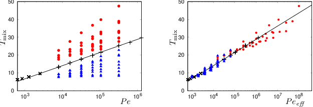
The evolution of the mixing time of the colloids, $T_{mix,c}$, as a function of $Pe_{c}$ is displayed in figure (2, left) for all simulations with $D_{\mathrm{dp}}^{2}/D_{c}D_{s}>1$, and different symbols for the salt-attracting case (circles) and the salt-reppelling case (triangles). The solid line is a fit for the non-diffusiophoretic cases (salt or colloids without salt), defined as

for this particular flow.

As shown in figure (2, right), all values of the mixing time are found to follow well the curve obtained without diffusiophoresis when they are plotted as a function of the effective Péclet numbers $Pe_{\mathit{eff}}^{\mathit{attract}}=\frac{D_{\mathrm{dp}}^{2}}{D_{c}D_{s}}\,Pe$ for “salt-attracting” case, and $Pe_{\mathit{eff}}^{\mathit{repell}}=\frac{D_{c}D_{s}}{D_{\mathrm{dp}}^{2}}\,Pe$ for the “salt-repelling” case; note also that the effective Péclet number varies here over five orders of magnitude.

The validity of our analysis can be further checked by focusing on the salt-repelling case. In that case the relation (36) is indeed equivalent to having an effective diffusivity

or an effective Péclet number independent of $D_{c}$, such that the mixing time becomes independent of $Pe_{c}$. Figure 3 displays $T_{mix,c}$, as a function of $Pe_{c}$ in the salt-repelling case ($D_{\mathrm{dp}}<0$), linking the data points corresponding to the same values of $D_{\mathrm{dp}}$ and $D_{s}$. As predicted, the different curves seem to exhibit a plateau when $Pe_{c}$ is large enough so that ${D_{\mathrm{dp}}^{2}}/{D_{c}D_{s}}\geq 10$ (filled symbol).

References

- Abécassis et al. (2009) Abécassis, B., Cottin-Bizonne, C., Ybert, C., Ajdari, A. & Bocquet, L. 2009 Osmotic manipulation of particles for microfluidic applications. New Journal of Physics 11 (7), 075022.
- Anderson (1989) Anderson, J. L. 1989 Colloid transport by interfacial forces. Annu. Rev. Fluid. Mech. 21, 61–99.
- Aris (1956) Aris, R. 1956 On the dispersion of a solute in a fluid flowing through a tube. Proceedings of the Royal Society of London A: Mathematical, Physical and Engineering Sciences 235 (1200), 67–77, arXiv: http://rspa.royalsocietypublishing.org/content/235/1200/67.full.pdf.
- Bakunin (2011) Bakunin, Oleg G., ed. 2011 Chaotic Flows. Springer.
- Banerjee et al. (2016) Banerjee, Anirudha, Williams, Ian, Azevedo, Rodrigo Nery, Helgeson, Matthew E. & Squires, Todd M. 2016 Soluto-inertial phenomena: Designing long-range, long-lasting, surface-specific interactions in suspensions. Proceedings of the National Academy of Sciences 113 (31), 8612–8617.
- Biferale et al. (1995) Biferale, L., Crisanti, A., Vergassola, M. & Vulpiani, A. 1995 Eddy diffusivities in scalar transport. Physics of Fluids 7 (11), 2725–2734.
- Birch et al. (2008) Birch, D.A., Young, W.R. & Franks, P.J.S. 2008 Thin layers of plankton: Formation by shear and death by diffusion. Deep Sea Research Part I: Oceanographic Research Papers 55 (3), 277 – 295.
- Deseigne et al. (2014) Deseigne, J., Cottin-Bizonne, C., Stroock, A. D., Bocquet, L. & Ybert, C. 2014 How a ”pinch of salt” can tune chaotic mixing of colloidal suspensions. Soft Matter 10, 4795–4799.
- Frish (1995) Frish, U. 1995 Turbulence-The Legacy of A. N. Kolmogorov.. Cambridge university press.
- Mauger et al. (2016) Mauger, Cyril, Volk, Romain, Machicoane, Nathanaël, Bourgoin, Michaël, Cottin-Bizonne, Cécile, Ybert, Christophe & Raynal, Florence 2016 Diffusiophoresis at the macroscale. Phys. Rev. Fluids 1, 034001.
- Metcalfe et al. (2012) Metcalfe, Guy, Speetjens, MFM, Lester, DR & Clercx, HJH 2012 Beyond passive: chaotic transport in stirred fluids. In Advances in Applied Mechanics, , vol. 45, pp. 109–188. Elsevier.
- Pierrehumbert (1994) Pierrehumbert, R. T. 1994 Tracer microstructure in the large-eddy dominated regime. Chaos, Solitons & Fractals 4 (6), 1091–1110.
- Pierrehumbert (2000) Pierrehumbert, R. T. 2000 Lattice models of advection-diffusion. Chaos 10 (1), 61–74.
- Ranz (1979) Ranz, W. E. 1979 Applications of a stretch model to mixing, diffusion, and reaction in laminar and turbulent flows. AIChE Journal 25 (41), 075022.
- Raynal et al. (2018) Raynal, Florence, Bourgoin, Mickael, Cottin-Bizonne, Cécile, Ybert, Christophe & Volk, Romain 2018 Advection and diffusion in a chemically induced compressible flow. Journal of Fluid Mechanics 847, 228–243.
- Raynal & Gence (1997) Raynal, F. & Gence, J.-N. 1997 Energy saving in chaotic laminar mixing. Int. J. Heat Mass Transfer 40 (14), 3267–3273.
- Schmidt et al. (2016) Schmidt, Lukas, Fouxon, Itzhak, Krug, Dominik, van Reeuwijk, Maarten & Holzner, Markus 2016 Clustering of particles in turbulence due to phoresis. Phys. Rev. E 93, 063110.
- Shukla et al. (2017) Shukla, Vishwanath, Volk, Romain, Bourgoin, Mickaël & Pumir, Alain 2017 Phoresis in turbulent flows. New Journal of Physics 19 (12), 123030.
- Sundararajan & Stroock (2012) Sundararajan, P. & Stroock, A. D. 2012 Transport phenomena in chaotic laminar flows. Annual Review of Fluid Mechanics 3, 473–493.
- Villermaux (2019) Villermaux, E. 2019 Mixing versus stirring. Annual Review of Fluid Mechanics 51, 245–273.
- Volk et al. (2014) Volk, R., Mauger, C., Bourgoin, M., Cottin-Bizonne, C., Ybert, C. & Raynal, F. 2014 Chaotic mixing in effective compressible flows. Phys. Rev. E 90, 013027.