跳到论文正文
W Papers独立论文阅读器 arXiv:1908.09141 论文正文 计算阅读时间 · 0%
引用这篇论文根据当前论文元数据生成,正式投稿前建议核对。


License: arXiv.org perpetual non-exclusive license
arXiv:1908.09141v2 [cond-mat.mes-hall] 07 Sep 2019

Chiral Pumping of Spin Waves

Tao Yu Affiliation: Kavli Institute of NanoScience, Delft University of Technology, 2628 CJ Delft, The Netherlands    Yaroslav M. Blanter Affiliation: Kavli Institute of NanoScience, Delft University of Technology, 2628 CJ Delft, The Netherlands    Gerrit E. W. Bauer Affiliation: Institute for Materials Research & WPI-AIMR & CSRN, Tohoku University, Sendai 980-8577, Japan Affiliation: Kavli Institute of NanoScience, Delft University of Technology, 2628 CJ Delft, The Netherlands
August 11, 2026
Abstract

We report a theory for the coherent and incoherent chiral pumping of spin waves into thin magnetic films through the dipolar coupling with a local magnetic transducer, such as a nanowire. The ferromagnetic resonance of the nanowire is broadened by the injection of unidirectional spin waves that generates a non-equilibrium magnetization in only half of the film. A temperature gradient between the local magnet and film leads to a unidirectional flow of incoherent magnons, i.e., a chiral spin Seebeck effect.

Introduction.—Magnonics and magnon spintronics are fields in which spin waves—the collective excitations of magnetic order—and their quanta, magnons, are studied with the purpose of using them as information carriers in low-power devices [1; 2; 3; 4]. Magnons carry angular momentum or “spin” by the precession direction around the equilibrium state. By angular momentum conservation the magnon spin couples to electromagnetic waves with only one polarization [5], which can be used to control spin waves [1; 2; 3; 4]. Surface spin waves or Damon-Eshbach (DE) modes have also a handedness or chirality, i.e. their linear momentum is fixed by the outer product of surface normal and magnetization direction [3; 7; 8; 9]. Alas, surface magnons have small group velocity, are dephased easily by surface roughness [4], and exist only in sufficiently thick magnetic films, which explains why they have not been employed for applications in magnonic devices [11].

The favored material for magnonics is the ferrimagnetic insulator yttrium iron garnet (YIG) with record low magnetization damping and high Curie temperature [12]. Spin waves in YIG films can be classified by the interaction that governs their dispersion as a function of wave vector to be of the dipolar, dipolar-exchange and exchange type with energies from a few GHz to many THz [1; 2; 3; 4]. Long-wavelength dipolar spin waves can be coherently excited by microwaves and travel over centimeters [13], but suffer from low group velocities. Exchange spin waves have much higher group velocity, but they can often be excited only incoherently by thermal or electric actuation via metallic contacts [9]. They are also scattered easily, leading to diffuse transport with reduced (micrometer) length scale. The dipolar-exchange spin waves are potentially most suitable for coherent information technologies by combining speed with long lifetime. Recently, short-wavelength dipolar-exchange spin waves have been coherently excited in magnetic films by attaching transducers in the form of thin and narrow ferromagnetic wires or wire arrays with high resonance frequencies [21; 16; 17; 18; 19; 20]. The dipolar interaction dominantly couples the transducer dynamics with the film, but in direct contact interface exchange and spin transfer torque may also play a role. Micromagnetic simulations [21] revealed that the AC dipolar field emitted by a magnetic wire antenna can excite spin waves in a magnetic film with magnetization normal to the wire, but no physical arguments or experiments supported this finding. Recently, almost perfectly chiral excitation of exchange spin waves was observed in thin YIG films with Co or Ni nanowire gratings with collinear magnetizations [23; 22].

The chiral excitation of spin waves [22] corresponds to a robust and switchable exchange magnon current generated by microwaves. The generation of DC currents by AC forces in the absence of a DC bias is referred to as “pumping” [24]. Spin pumping is the injection of a spin current by the magnetization dynamics of a magnet into a contact normal metal by the interface exchange interaction [25; 26]. We therefore call generation of unidirectional spin waves by the dynamics of a proximity magnetic wire chiral spin pumping. Here we present a semi-analytic theory of chiral spin pumping for arbitrary magnetic configurations. We distinguish coherent pumping by applied microwaves from the incoherent (thermal) pumping by a temperature difference, i.e. the chiral spin Seebeck effect [27; 28; 29; 30] as shown schematically in Fig. 1. The former has been studied by microwave transmission spectroscopy [23; 22]. Both effects can be observed also electrically via the inverse spin Hall effect in heavy metal contacts, but we focus here on the more efficient inductive detection scheme.

Chiral spin pumping turns out to be very anisotropic. When spin waves propagate perpendicular to the magnetization with opposite momenta, their dipolar fields vanish on opposite sides of the film; when propagating parallel to the magnetization, their dipolar field is chiral, i.e., polarization-momentum locked. Purely chiral coupling between magnons can be achieved in the former case without constraints on the degree of polarization of the local magnet. We also find that the pumping by dipolar interaction is chiral in both momentum and real space, i.e., in the configuration of Fig. 1 unidirectional spin waves are excited in half of the film.

Figure 1: Chiral Spin Seebeck effect. A thin non-magnetic spacer between the YIG film and Co nanowire (optionally) suppresses the exchange interaction. The effect is maximal for the antiparallel magnetization (see text). The magnitude of the magnon currents pumped into the ±𝐲^\pm\mathbf{\hat{y}} directions is indicated by the size of the red arrows. Another Co nanowire (the blue one) is suggested to detect the population or temperature of magnon with long-wavelength.

Origin of the chiral coupling.—The dynamic dipolar coupling of magnetization 𝐌~\mathbf{\tilde{M}} of the local magnet with that of a film 𝐌\mathbf{M} by the Zeeman interaction with the respective dipolar magnetic fields 𝐡\mathbf{h} and 𝐡~\mathbf{\tilde{h}} [31]

H^int/μ0=−∫𝐌~(𝐫,t)⋅𝐡(𝐫,t)d𝐫=−∫𝐌(𝐫,t)⋅𝐡~(𝐫,t)d𝐫,\hat{H}_{\mathrm{int}}/\mu_{0}=-\int\mathbf{\tilde{M}}(\mathbf{r},t)\cdot\mathbf{h}(\mathbf{r},t)d\mathbf{r}=-\int\mathbf{M}(\mathbf{r},t)\cdot\mathbf{\tilde{h}}(\mathbf{r},t)d\mathbf{r}, (1)

where μ0\mu_{0} is the vacuum permeability. We focus here on circularly polarized exchange spin waves in a magnetic film with thickness ss at frequency ω\omega and in-plane wave vector 𝐤=ky​𝐲^+kz​𝐳^\mathbf{k}=k_{y}\hat{\mathbf{y}}+k_{z}\hat{\mathbf{z}} in the coordinate system defined in Fig. 1 (the general case is treated in the Supplemental Material (SM) Sec. I.A [33]). Classically, Mx​(𝐫,t)=mR𝐤​(x)​cos⁡(𝐤⋅𝝆−ω​t)M_{x}(\mathbf{r},t)=m_{R}^{\mathbf{k}}(x)\cos(\mathbf{k}\cdot\boldsymbol{\rho}-\omega t) and My​(𝐫,t)≡−mR𝐤​(x)​sin⁡(𝐤⋅𝝆−ω​t)M_{y}(\mathbf{r},t)\equiv-m_{R}^{\mathbf{k}}(x)\sin(\mathbf{k}\cdot\boldsymbol{\rho}-\omega t) describe the precession around the equilibrium magnetization modulated in the 𝐳^\hat{\mathbf{z}}-direction, where mR𝐤​(x)m_{R}^{\mathbf{k}}(x) is the time-independent amplitude normal to the film and 𝝆=y​𝐲^+z​𝐳^.\boldsymbol{\rho}=y\hat{\mathbf{y}}+z\hat{\mathbf{z}}. The dipolar field outside the film generated by the spin waves

hβ​(𝐫,t)=14​π​∂β∂α∫d​𝐫′​Mα​(𝐫′,t)|𝐫−𝐫′|,h_{\beta}(\mathbf{r},t)=\frac{1}{4\pi}\partial_{\beta}\partial_{\alpha}\int d\mathbf{r}^{\prime}\frac{M_{\alpha}(\mathbf{r}^{\prime},t)}{|\mathbf{r}-\mathbf{r}^{\prime}|}, (2)

in the summation convention over repeated Cartesian indices α,β={x,y,z}\alpha,\beta=\{x,y,z\} [31], becomes

(hx​(𝐫,t)hy​(𝐫,t)hz​(𝐫,t))\displaystyle\left(\begin{array}[c]{c}h_{x}(\mathbf{r},t)\\ h_{y}(\mathbf{r},t)\\ h_{z}(\mathbf{r},t)\end{array}\right) =((k+η​ky)​cos⁡(𝐤⋅𝝆−ω​t)(ky2k+η​ky)​sin⁡(𝐤⋅𝝆−ω​t)kz​(kyk+η)​sin⁡(𝐤⋅𝝆−ω​t))\displaystyle=\left(\begin{array}[c]{c}\left(k+\eta k_{y}\right)\cos\left(\mathbf{k}\cdot\boldsymbol{\rho}-\omega t\right)\\ \left(\frac{k_{y}^{2}}{k}+\eta k_{y}\right)\sin\left(\mathbf{k}\cdot\boldsymbol{\rho}-\omega t\right)\\ k_{z}\left(\frac{k_{y}}{k}+\eta\right)\sin\left(\mathbf{k}\cdot\boldsymbol{\rho}-\omega t\right)\end{array}\right)
×12​e−η​k​x​∫d​x′​mR𝐤​(x′)​eη​k​x′,\displaystyle\times\frac{1}{2}e^{-\eta kx}\int dx^{\prime}m_{R}^{\mathbf{k}}\left(x^{\prime}\right)e^{\eta kx^{\prime}}, (9)

where the spatial integral is over the film thickness ss. x>0x>0 (x<−sx<-s) is the case with the dipolar field above (below) the film and η=1\eta=1 (−1-1) when x>0x>0 (x<−sx<-s), k=|𝐤|k=\left|\mathbf{k}\right|. The interaction Hamiltonian (1) for a wire with thickness dd and width ww [31] reduced to

H^int(t)=−μ0∫0dM~^β(x,𝝆,t)h^β(x,𝝆,t)dxd𝝆.\hat{H}_{\mathrm{int}}(t)=-\mu_{0}\int_{0}^{d}\hat{\tilde{M}}_{\beta}(x,\boldsymbol{\rho},t)\hat{h}_{\beta}(x,\boldsymbol{\rho},t)dxd\boldsymbol{\bf\rho}. (10)

The spin waves in the film with kz=0k_{z}=0 propagate normal to the wire with dipolar field hz=0h_{z}=0. The distribution of the dipolar field above and below the film then strongly depends on the wave vector direction: the dipolar field generated by the right (left) moving spin waves vanishes below (above) the film [22] and precesses in the opposite direction of the magnetization as sketched in Fig. 2. The magnetization in the wire precesses in a direction governed by the magnetization direction and couples only to spin waves with finite dipolar field amplitude in the wire and matched precession [22; 23]. We thus understand without calculations that the dipolar coupling is chiral and the time-averaged coupling strength is maximized when the magnetizations of the film and wire are antiparallel.

Figure 2: Half-space dipolar fields generated by spin waves propagating normal to the (equilibrium) magnetization of an in-plane magnetized film (𝐌s|𝐳^\mathbf{M}_{s}\parallel\hat{\mathbf{z}}). The fat black arrow in (a) and red arrows in (b) indicate the spin wave propagation direction. The black (red) circles are the precession cones of the film magnetization (corresponding dipolar field) and precession direction is indicated by thin blue arrows.

Spin waves in the film propagating parallel to the magnetization (ky=0→hy=0k_{y}=0\rightarrow h_{y}=0) may also couple chirally to the local magnet, but by a different mechanism. According to Eq. (9), hx∝|kz|​cos⁡(kz​z−ω​t)h_{x}\propto\left|k_{z}\right|\cos\left(k_{z}z-\omega t\right) and hz∝η​kz​sin⁡(kz​z−ω​t)h_{z}\propto\eta k_{z}\sin\left(k_{z}z-\omega t\right). Above the film, the dipolar fields with positive (negative) kzk_{z} are left (right) circularly polarized, respectively, while below the film, the polarizations are reversed. These spin waves couple with the magnet on one side of the film only when its transverse magnetization dynamics is right or left circularly polarized [21].

A circularly polarized uniform precession in the nanowire always couples chirally with the spin waves in the film (see SM Secs. I.B and II [33]) for all angles between magnetizations in film and nanowire irrespective of their polarization. When the nanowire Kittel mode is elliptical, the directionality vanishes for one specific angle θc\theta_{c}. When the nanowire Kittel mode is fully circularly polarized, the coupling strength vanishes and the critical angle θc=0\theta_{c}=0. With w>dw>d and weak magnetic field bias, θc≃arccos⁡(d/w)\theta_{c}\simeq\arccos\left(\sqrt{d/w}\right) (see SM Sec. II [33]) and the chirality can be controlled by weak in-plane magnetic fields.

General formalism.—Here we formulate the general problem of the dynamic dipolar coupling between a nanowire with equilibrium magnetization at an angle θ\theta that is in contact with an extended thin magnetic film. At resonance, microwaves populate preferentially the collective (“Kittel”) modes [32], while a finite temperature populates all magnon modes with a Planck distribution. We focus here on the collinear (parallel and antiparallel) configurations, deferring the derivations and discussions of general situations to the SM Sec. II [33]. For convenience, we formulate the problem in second quantization.

For sufficiently small amplitudes, the Cartesian components β∈{x,y}\beta\in\left\{x,y\right\} of the magnetization dynamics of film (𝐌^\mathbf{\hat{M}}) and nanowire (𝐌~^\mathbf{\hat{\tilde{M}}}) can be expanded into magnon creation and annihilation operators [34; 35; 4],

M^β​(𝐫)\displaystyle\hat{M}_{\beta}(\mathbf{r}) =−2​Ms​γ​ℏ∑𝐤[mβ(𝐤)(x)ei​𝐤⋅𝝆α^𝐤+h.c.],\displaystyle=-\sqrt{2M_{s}\gamma\hbar}\sum_{\mathbf{k}}\left[m_{\beta}^{\left(\mathbf{k}\right)}(x)e^{i{\mathbf{k}}\cdot\boldsymbol{\rho}}\hat{\alpha}_{\mathbf{k}}+\mathrm{h.c.}\right],
M~^β​(𝐫)\displaystyle\hat{\tilde{M}}_{\beta}(\mathbf{r}) =−2​M~s​γ​ℏ∑kz[m~β(kz)(x,y)ei​kz​zβ^kz+h.c.],\displaystyle=-\sqrt{2\tilde{M}_{s}\gamma\hbar}\sum_{k_{z}}\left[\tilde{m}_{\beta}^{(k_{z})}(x,y)e^{ik_{z}z}\hat{\beta}_{k_{z}}+\mathrm{h.c.}\right], (11)

where MsM_{s} and M~s\tilde{M}_{s} are the saturation magnetizations, −γ-\gamma is the gyromagnetic ratio, mβ(𝐤)​(x)m_{\beta}^{\left(\mathbf{k}\right)}(x) and m~β(kz)​(x,y)\tilde{m}_{\beta}^{(k_{z})}(x,y) are the spin wave amplitudes across the film and nanowire, and α^𝐤\hat{\alpha}_{\mathbf{k}} and β^kz\hat{\beta}_{k_{z}} denote the magnon (annihilation) operator in the film and nanowire, respectively.

We are mainly interested in high-quality ultrathin films and nanowires with s,d≳𝒪⁡(10​nm)s,d\gtrsim\mathcal{O}\left(10~\mathrm{nm}\right) and nanowire width w≳𝒪⁡(50​nm)w\gtrsim\mathcal{O}\left(50~\mathrm{nm}\right), such that the magnetization across the film and nanowire (centered at y0​𝐲^y_{0}\hat{\mathbf{y}}) are nearly homogeneous: mβ(𝐤)​(x)≈mβ(𝐤)​Θ​(−x)​Θ​(x+s)m_{\beta}^{\left(\mathbf{k}\right)}(x)\approx m_{\beta}^{\left(\mathbf{k}\right)}\Theta(-x)\Theta(x+s) and m~β(kz)​(x,y)≈m~β(kz)​Θ​(x)​Θ​(−x+d)​Θ​(y−y0+w/2)​Θ​(−y+y0+w/2)\tilde{m}_{\beta}^{\left(k_{z}\right)}(x,y)\approx\tilde{m}_{\beta}^{\left(k_{z}\right)}\Theta(x)\Theta(-x+d)\Theta(y-y_{0}+w/2)\Theta(-y+y_{0}+w/2), with Θ⁡(x)\Theta(x) the Heaviside step function [22; 23; 20]. Disregarding higher magnon subbands turns out to be a good approximation even at higher temperatures because of the strong mode selectivity of the dipolar coupling [33]. Here we disregard interface exchange, which appears to play only a minor role [22; 23]. The system Hamiltonian then becomes

H^/ℏ\displaystyle\hat{H}/\hbar =∑𝐤ω𝐤​α^𝐤†​α^𝐤+∑kzω~kz​β^kz†​β^kz\displaystyle=\sum_{\mathbf{k}}\omega_{\mathbf{k}}\hat{\alpha}_{\mathbf{k}}^{\dagger}\hat{\alpha}_{\mathbf{k}}+\sum_{k_{z}}\tilde{\omega}_{k_{z}}\hat{\beta}_{k_{z}}^{\dagger}\hat{\beta}_{k_{z}}
+∑𝐤(g𝐤e−i​ky​y0α^𝐤†β^kz+g𝐤∗ei​ky​y0β^kz†α^𝐤),\displaystyle+\sum_{\mathbf{k}}\left(g_{\mathbf{k}}e^{-ik_{y}y_{0}}\hat{\alpha}_{\mathbf{k}}^{\dagger}\hat{\beta}_{k_{z}}+g_{\mathbf{k}}^{\ast}e^{ik_{y}y_{0}}\hat{\beta}_{k_{z}}^{\dagger}\hat{\alpha}_{\mathbf{k}}\right), (12)

where ω𝐤\omega_{\mathbf{k}} and ω~kz\tilde{\omega}_{k_{z}} are the frequencies of spin waves in the film and nanowire and, with Eqs. (2), (10) and (11), the coupling

g𝐤=F(𝐤)(mx(𝐤)∗,my(𝐤)∗)(|𝐤|i​kyi​ky−ky2/|𝐤|)(m~x(kz)m~y(kz)),g_{\mathbf{k}}=F(\mathbf{k})\left(m_{x}^{(\mathbf{k})\ast},m_{y}^{(\mathbf{k})\ast}\right)\left(\begin{array}[c]{cc}|\mathbf{k}|&ik_{y}\\ ik_{y}&-k_{y}^{2}/|\mathbf{k}|\end{array}\right)\left(\begin{array}[c]{c}\tilde{m}_{x}^{(k_{z})}\\ \tilde{m}_{y}^{(k_{z})}\end{array}\right), (13)

with F⁡(𝐤)=−μ0​γ​Ms​M~s/L​ϕ​(𝐤)F(\mathbf{k})=-\mu_{0}\gamma\sqrt{M_{s}\tilde{M}_{s}/L}\phi\left(\mathbf{k}\right). The form factor ϕ⁡(𝐤)=2​sin⁡(ky​w/2)​(1−e−k​d)​(1−e−k​s)/(ky​k2)\phi\left(\mathbf{k}\right)=2\sin(k_{y}w/2)(1-e^{-kd})(1-e^{-ks})/(k_{y}{k^{2}}) couples spin waves with wavelengths of the order of the nanowire width (mode selection) and lim𝐤→0ϕ⁡(𝐤)=w​s​d\lim_{\mathbf{\ k}\rightarrow 0}\phi\left(\mathbf{k}\right)=wsd. Exchange waves are right-circularly polarized with my(ky)=i​mx(ky)m_{y}^{(k_{y})}=im_{x}^{(k_{y})} and the coupling is perfectly chiral g−|ky|=0g_{-|k_{y}|}=0 (refer to Fig. 2).

The linear response to microwave and thermal excitations can be described by the input-output theory [36; 37] and by a Kubo formula (see SM Sec. III [33]). Let p^kz​(t)=∫p^kz​(ω)​e−i​ω​t​𝑑ω/(2​π)\hat{p}_{k_{z}}(t)=\int\hat{p}_{k_{z}}(\omega)e^{-i\omega t}d\omega/(2\pi) be a microwave photon input with magnetic field ∝(p^kz​(t)+p^kz†​(t))\propto(\hat{p}_{k_{z}}(t)+\hat{p}_{k_{z}}^{\dagger}(t)) centered at the frequency ω~kz:\tilde{\omega}_{k_{z}}: ⟨p^kz​(ω)⟩→2​π​𝒟​δ​(ω−ω~kz)\langle\hat{p}_{k_{z}}(\omega)\rangle\rightarrow 2\pi\mathit{\mathcal{D}}\delta(\omega-\tilde{\omega}_{k_{z}}) with amplitude 𝒟\mathcal{D}, the equations of motion are [36; 37]

d​β^kzd​t\displaystyle\frac{d\hat{\beta}_{k_{z}}}{dt} =−i​ω~kz​β^kz​(t)−∑kyi​g𝐤∗​ei​ky​y0​α^𝐤​(t)\displaystyle=-i\tilde{\omega}_{k_{z}}\hat{\beta}_{k_{z}}(t)-\sum_{k_{y}}ig_{\mathbf{k}}^{\ast}e^{ik_{y}y_{0}}\hat{\alpha}_{\mathbf{k}}(t)
−(κ~kz2+ζkz2)​β^kz​(t)−κ~kz​N~^kz​(t)−ζkz​p^kz​(t),\displaystyle-\left(\frac{\tilde{\kappa}_{k_{z}}}{2}+\frac{\zeta_{k_{z}}}{2}\right)\hat{\beta}_{k_{z}}(t)-\sqrt{\tilde{\kappa}_{k_{z}}}\hat{\tilde{N}}_{k_{z}}(t)-\sqrt{\zeta_{k_{z}}}\hat{p}_{k_{z}}(t), (14)
d​α^𝐤d​t\displaystyle\frac{d\hat{\alpha}_{\mathbf{k}}}{dt} =−i​ω𝐤​α^𝐤​(t)−i​g𝐤​e−i​ky​y0​β^kz​(t)−κ𝐤2​α^𝐤​(t)\displaystyle=-i\omega_{\mathbf{k}}\hat{\alpha}_{\mathbf{k}}(t)-ig_{\mathbf{k}}e^{-ik_{y}y_{0}}\hat{\beta}_{k_{z}}(t)-\frac{\kappa_{\mathbf{k}}}{2}\hat{\alpha}_{\mathbf{k}}(t)
−κ𝐤​N^𝐤​(t),\displaystyle-\sqrt{\kappa_{\mathbf{k}}}\hat{N}_{\mathbf{k}}(t), (15)

where κ~kz≡2​χ~​ω~kz\tilde{\kappa}_{k_{z}}\equiv 2\tilde{\chi}\tilde{\omega}_{k_{z}}\ (κ𝐤≡2​χ​ω𝐤\kappa_{\mathbf{k}}\equiv 2\chi\omega_{\mathbf{k}}) is the damping rates in terms of the Gilbert damping constant χ~​(χ)\tilde{\chi}\ (\chi) in the nanowire (film) and ζkz\zeta_{k_{z}} is the radiative damping. The thermal environment of the magnetic film causes fluctuations N^𝐤\hat{N}_{\mathbf{k}} [37] generated by a Markovian process that obeys the (quantum) fluctuation-dissipation theorem with ⟨N^𝐤⟩=0\langle{\hat{N}_{\mathbf{k}}}\rangle=0 and ⟨N^𝐤†​(t)​N^𝐤′​(t′)⟩=n𝐤​δ​(t−t′)​δ𝐤𝐤′\langle{\hat{N}_{\mathbf{k}}^{\dagger}(t)\hat{N}_{\mathbf{k}^{\prime}}(t^{\prime})}\rangle=n_{\mathbf{k}}\delta(t-t^{\prime})\delta_{\mathbf{k}\mathbf{k}^{\prime}}. n𝐤=1/{exp⁡[ℏ​ω𝐤/(kB​T2)]−1}n_{\mathbf{k}}=1/\left\{\exp\left[{\hbar\omega_{\mathbf{k}}}/({k_{B}T_{2}})\right]-1\right\} is the magnon population at temperature T2T_{2} of film, and kB​T2k_{B}T_{2} should be larger than ℏ​ω𝐤\hbar\omega_{\mathbf{k}}. In frequency space with A^​(t)=∫𝑑ω/(2​π)​A^​(ω)​e−i​ω​t\hat{A}(t)=\int d\omega/({2\pi})\hat{A}(\omega)e^{-i\omega t}, ⟨N^𝐤†​(ω)​N^𝐤′​(ω′)⟩=2​π​δ​(ω−ω′)​n𝐤​δ𝐤𝐤′\left\langle\hat{N}_{\mathbf{k}}^{\dagger}(\omega)\hat{N}_{\mathbf{k}^{\prime}}(\omega^{\prime})\right\rangle=2\pi\delta(\omega-\omega^{\prime})n_{\mathbf{k}}\delta_{\mathbf{k}\mathbf{k}^{\prime}}. The thermal fluctuations N~^kz\hat{\tilde{N}}_{k_{z}} in the nanowire are characterized by a different temperature T1T_{1} and thermal magnon distribution n~kz=1/{exp⁡[ℏ​ω~kz/(kB​T1)]−1}\tilde{n}_{k_{z}}=1/\left\{\exp\left[{\hbar\tilde{\omega}_{k_{z}}}/({k_{B}T_{1}})\right]-1\right\}. The solutions

β^kz​(ω)\displaystyle\hat{\beta}_{k_{z}}(\omega) =i​∑kyγ𝐤​G𝐤​N^𝐤​(ω)−κ~kz​N~^kz​(ω)−ζkz​p^kz​(ω)−i⁡(ω−ω~kz)+κ~kz2+ζkz2+i​∑ky|g𝐤|2​G𝐤​(ω),\displaystyle=\frac{i\sum\limits_{k_{y}}\gamma_{\mathbf{k}}G_{\mathbf{k}}\hat{N}_{\mathbf{k}}(\omega)-\sqrt{\tilde{\kappa}_{k_{z}}}\hat{\tilde{N}}_{k_{z}}(\omega)-\sqrt{\zeta_{k_{z}}}\hat{p}_{k_{z}}(\omega)}{-i(\omega-\tilde{\omega}_{k_{z}})+\frac{\tilde{\kappa}_{k_{z}}}{2}+\frac{\zeta_{k_{z}}}{2}+i\sum_{k_{y}}|g_{\mathbf{k}}|^{2}G_{\mathbf{k}}\left(\omega\right)},
α^𝐤​(ω)\displaystyle\hat{\alpha}_{\mathbf{k}}(\omega) =G𝐤​(ω)​(g𝐤​e−i​ky​y0​β^kz​(ω)−i​κ𝐤​N^𝐤​(ω)),\displaystyle=G_{\mathbf{k}}\left(\omega\right)\left(g_{\mathbf{k}}e^{-ik_{y}y_{0}}\hat{\beta}_{k_{z}}(\omega)-i\sqrt{\kappa_{\mathbf{k}}}\hat{N}_{\mathbf{k}}(\omega)\right), (16)

with Green function G𝐤​(ω)=((ω−ω𝐤)+i​κ𝐤/2)−1G_{\mathbf{k}}\left(\omega\right)=\left((\omega-\omega_{\mathbf{k}})+i\kappa_{\mathbf{k}}/2\right)^{-1} and γ𝐤=i​g𝐤∗​ei​ky​y0​κ𝐤\gamma_{\mathbf{k}}=ig_{\mathbf{k}}^{\ast}e^{ik_{y}y_{0}}\sqrt{\kappa_{\mathbf{k}}}, reveal that the thermal fluctuations in both wire (N~^kz\hat{\tilde{N}}_{k_{z}}) and film (N^𝐤\hat{N}_{\mathbf{k}}) affect β^kz​(ω)\hat{\beta}_{k_{z}}(\omega). Moreover, the interaction enhances the damping of nanowire spin waves by δ​κ~kz=2​π​∑ky|g𝐤|2​δ​(ω~kz−ω𝐤)\delta\tilde{\kappa}_{k_{z}}=2\pi\sum_{k_{y}}|g_{\mathbf{k}}|^{2}\delta(\tilde{\omega}_{k_{z}}-\omega_{\mathbf{k}}) to κ~kz′\tilde{\kappa}_{k_{z}}^{\prime}, and shifts the frequency to ω~kz′\tilde{\omega}_{k_{z}}^{\prime}. Chiral pumping can be realized by coherent microwave excitation or the incoherent excitation by a temperature difference between the local magnet and film, as shown in the following.

Coherent chiral pumping.—A uniform microwave field excites only the Kittel mode (kz=0k_{z}=0) in the nanowire but not the film. Spin waves in the film with finite ky≡qk_{y}\equiv q are excited indirectly by the inhomogeneous stray field of the wire. The coherent chiral pumping by microwaves at thermal equilibrium with T1=T2≡T0T_{1}=T_{2}\equiv T_{0} in the time and wave number domain reads

α^q​(t)=∫d​ω2​π​e−i​ω​t​i​gq​e−i​q​y0−i⁡(ω−ωq)+κq2​ζ0​p^0​(ω)−i⁡(ω−ω~0′)+κ~0′2+ζ02.\hat{\alpha}_{q}(t)=\int\frac{d\omega}{2\pi}\frac{e^{-i\omega t}ig_{q}e^{-iqy_{0}}}{-i(\omega-\omega_{q})+\frac{\kappa_{q}}{2}}\frac{\sqrt{\zeta_{0}}\hat{p}_{0}(\omega)}{-i(\omega-\tilde{\omega}_{0}^{\prime})+\frac{\tilde{\kappa}_{0}^{\prime}}{2}+\frac{\zeta_{0}}{2}}. (17)

Since the magnons are coherently excited their number is ⟨α^q†​(t)​α^q​(t)⟩=⟨α^q†​(t)⟩​⟨α^q​(t)⟩\langle\hat{\alpha}_{q}^{\dagger}(t)\hat{\alpha}_{q}(t)\rangle=\langle\hat{\alpha}_{q}^{\dagger}(t)\rangle\langle\hat{\alpha}_{q}(t)\rangle. In the absence of damping, κq\kappa_{q} is a positive infinitesimal that safeguards causality. A resonant input ⟨p^0⟩=2​π​𝒟​δ​(ω−ω~0)\langle\hat{p}_{0}\rangle=2\pi\mathcal{D}\delta(\omega-\tilde{\omega}_{0}) excites a film magnetization in position space

δ​Mβ​(𝐫,t)\displaystyle\delta{M}_{\beta}(\mathbf{r},t) =2​Ms​γ​ℏ​𝒟​e−i​ω~0​t​ζ0−i⁡(ω~0−ω~0′)+(κ~0′+ζ0)/2\displaystyle=\sqrt{2M_{s}\gamma\hbar}\mathcal{D}\frac{e^{-i\tilde{\omega}_{0}t}\sqrt{\zeta_{0}}}{-i(\tilde{\omega}_{0}-\tilde{\omega}_{0}^{\prime})+(\tilde{\kappa}_{0}^{\prime}+\zeta_{0})/2}
×∑qmβ(q)​(x)​gq​ei​q​(y−y0)(ω~0−ωq)+i​κq/2+h.c..\displaystyle\times\sum_{q}m_{\beta}^{\left(q\right)}(x)\frac{g_{q}e^{iq(y-y_{0})}}{(\tilde{\omega}_{0}-\omega_{q})+i\kappa_{q}/2}+\mathrm{h.c.}. (18)

The denominator ω~0−ωq+i​κq/2\tilde{\omega}_{0}-\omega_{q}+i\kappa_{q}/2\ vanishes for q±=±(q∗+i​δΓ)q_{\pm}=\pm(q_{\ast}+i\delta_{\Gamma}) in the complex plane with q∗>0q_{\ast}>0 and inverse propagation length δΓ\delta_{\Gamma}. Closing the contour, we obtain

δ​Mβ​(𝐫)\displaystyle\delta{M}_{\beta}(\mathbf{r}) =2​Ms​γ​ℏ​𝒟​1vq∗​e−i​ω~0​t​ζ0(ω~0−ω~0′)+i⁡(κ~0′+ζ0)/2\displaystyle=\sqrt{2M_{s}\gamma\hbar}\mathcal{D}\frac{1}{v_{q_{\ast}}}\frac{e^{-i\tilde{\omega}_{0}t}\sqrt{\zeta_{0}}}{(\tilde{\omega}_{0}-\tilde{\omega}_{0}^{\prime})+i(\tilde{\kappa}_{0}^{\prime}+\zeta_{0})/2}
×{mβ(q∗)​(x)​gq∗​ei​q+​(y−y0)+h.c.mβ(−q∗)​(x)​g−q∗​ei​q−​(y−y0)+h.c.​ for ​y>y0y<y0,\displaystyle\times\left\{\begin{array}[c]{c}m_{\beta}^{(q_{\ast})}(x)g_{q_{\ast}}e^{iq_{+}(y-y_{0})}+\mathrm{h.c.}\\ m_{\beta}^{(-q_{\ast})}(x)g_{-q_{\ast}}e^{iq_{-}(y-y_{0})}+\mathrm{h.c.}\end{array}\text{ for }\begin{array}[c]{c}y>y_{0}\\ y<y_{0}\end{array}\right.,

where vq∗=∂ωq/∂q|q∗v_{q_{\ast}}=\left.\partial\omega_{q}/\partial q\right|_{q_{\ast}} is the magnon group velocity. For perfect chiral coupling g−q∗=0g_{-q_{\ast}}=0 only the magnetization in half space y>y0y>y_{0} can be excited, which implies handedness also in position space.

The coherent chiral pumping can be directly observed by microwave transmission spectra [16; 19; 20]. We let here two nanowires at 𝐫1=R1​𝐲^\mathbf{r}_{1}=R_{1}\hat{\mathbf{y}} and 𝐫2=R2​𝐲^\mathbf{r}_{2}=R_{2}\hat{\mathbf{y}} act as excitation and detection transducers. The spin wave transmission amplitude as derived and calculated in the SM Sec. IV [33] reads

S21​(ω)=[1−S11​(ω)]​∑qi​Gq​(ω)​|gq|2​ei​q​(R2−R1)−i⁡(ω−ω~0)+κ~0/2+i​∑qGq​(ω)​|gq|2,S_{21}(\omega)=\frac{\left[1-S_{11}(\omega)\right]\sum_{q}iG_{q}\left(\omega\right)|g_{q}|^{2}e^{iq(R_{2}-R_{1})}}{-i(\omega-\tilde{\omega}_{0})+\tilde{\kappa}_{0}/2+i\sum_{q}G_{q}\left(\omega\right)|g_{q}|^{2}}, (23)

and the reflection amplitude S11​(ω)S_{11}(\omega) is given in the SM. Chirality enters via the phase factor ei​q​(R2−R1)e^{iq(R_{2}-R_{1})}: When g−|q|=0g_{-|q|}=0, spin and microwaves are transmitted from 1 to 2 only when R2>R1R_{2}>R_{1}.

Incoherent chiral pumping.—Spin waves can be incoherently excited by locally heating the nanowire, e.g. by the Joule heating due to an applied current [9]. In the absence of microwaves p^kz=0\hat{p}_{k_{z}}=0, the magnon distribution of the film reads

f⁡(𝐤)\displaystyle f(\mathbf{k}) ≡⟨α^𝐤†​(t)​α^𝐤​(t)⟩\displaystyle\equiv\langle\hat{\alpha}_{\mathbf{k}}^{\dagger}(t)\hat{\alpha}_{\mathbf{k}}(t)\rangle
=n𝐤+|g𝐤|2(ω𝐤−ω~kz′)2+(κ~kz′/2)2​κ~kzκ𝐤​(n~kz−n𝐤).\displaystyle=n_{\mathbf{k}}+\frac{|g_{\mathbf{k}}|^{2}}{(\omega_{\mathbf{k}}-\tilde{\omega}_{k_{z}}^{\prime})^{2}+(\tilde{\kappa}_{k_{z}}^{\prime}/2)^{2}}\frac{\tilde{\kappa}_{k_{z}}}{\kappa_{\mathbf{k}}}\left(\tilde{n}_{k_{z}}-n_{\mathbf{k}}\right). (24)

When T1>T2T_{1}>T_{2}, magnons are injected from the local magnet into the film. When the coupling is chiral with g𝐤≠g−𝐤g_{\mathbf{k}}\neq g_{-\mathbf{k}}, the distribution of magnons is asymmetric, f⁡(𝐤)≠f⁡(−𝐤)f(\mathbf{k})\neq f(-\mathbf{k}), i.e. carries a unidirectional spin current I∝∑𝐤v𝐤​f​(𝐤)I\propto\sum_{\mathbf{k}}v_{\mathbf{k}}f(\mathbf{k}), which in turn generates a magnon accumulation in the detector magnet.

All occupied modes in the local magnet contribute to the excitation of the film. In position space

α^​(𝝆,t)=∫d​ω2​π​e−i​ω​t​∑𝐤ei​𝐤⋅𝝆​α^𝐤​(ω),\hat{\alpha}(\boldsymbol{\rho},t)=\int\frac{d\omega}{2\pi}e^{-i\omega t}\sum_{\mathbf{k}}e^{i\mathbf{k}\cdot\boldsymbol{\rho}}\hat{\alpha}_{\mathbf{k}}(\omega), (25)

and the excited magnon density for y>y0y>y_{0} in a high-quality film with κ𝐤→0+\kappa_{\mathbf{k}}\rightarrow 0_{+} reads

δ​ρ>≡⟨α^†​(𝝆,t)​α^​(𝝆,t)⟩|y>y0−∑𝐤n𝐤\displaystyle\delta\rho_{>}\equiv\left\langle\hat{\alpha}^{\dagger}(\boldsymbol{\rho},t)\hat{\alpha}(\boldsymbol{\rho},t)\right\rangle|_{y>y_{0}}-\sum_{\mathbf{k}}n_{\mathbf{k}}
=∑kz∫d​ω2​π​(n~kz−n𝐤ω)​|g𝐤ω|2v𝐤ω2​κ~kz(ω−ω~kz′)2+(κ~kz′/2)2,\displaystyle=\sum_{k_{z}}\int\frac{d\omega}{2\pi}(\tilde{n}_{k_{z}}-n_{\mathbf{k}_{\omega}})\frac{|g_{\mathbf{k}_{\omega}}|^{2}}{v_{\mathbf{k}_{\omega}}^{2}}\frac{\tilde{\kappa}_{k_{z}}}{(\omega-\tilde{\omega}_{k_{z}}^{\prime})^{2}+(\tilde{\kappa}_{k_{z}}^{\prime}/2)^{2}}, (26)

where 𝐤ω=qω​𝐲^+kz​𝐳^\mathbf{k}_{\omega}=q_{\omega}\hat{\mathbf{y}}+k_{z}\hat{\mathbf{z}} and qωq_{\omega} is the positive root of ωqω,kz=ω\omega_{q_{\omega},k_{z}}=\omega. For weak magnetic damping in the wire κ~m≪ω~m\tilde{\kappa}_{m}\ll\tilde{\omega}_{m}, the r.h.s reduces to δ​ρ>≈∑kz(|gq∗,kz|2/vq∗,kz2)​(n~kz−nq∗,kz)\delta\rho_{>}\approx\sum_{k_{z}}\left({|g_{q_{\ast},k_{z}}|^{2}}/{v_{q_{\ast},k_{z}}^{2}}\right)(\tilde{n}_{k_{z}}-n_{q_{\ast},k_{z}}) and ωq∗,kz=ω~kz\omega_{q_{\ast},k_{z}}=\tilde{\omega}_{k_{z}}. For y<y0y<y_{0}, δ​ρ<≈∑kz(|g−q∗,kz|2/vq∗,kz2)​(n~kz−nq∗,kz)≠δ​ρ>\delta\rho_{<}\approx\sum_{k_{z}}\left({|g_{-q_{\ast},k_{z}}|^{2}}/{v_{q_{\ast},k_{z}}^{2}}\right)(\tilde{n}_{k_{z}}-n_{q_{\ast},k_{z}})\neq\delta\rho_{>}. We conclude that the thermal injection via chiral coupling leads to different magnon densities on both sides of the nanowire. This is a chiral equivalent of the conventional spin Seebeck effect [27; 28; 29; 30].

The chiral pumping of magnons can be detected inductively via microwave emission of a second magnetic wire, by Brillouin light scattering [38; 23], NV center magnetometry [39], and electrically by the inverse spin Hall effect [9]. The incoherent excitation couples strongly only with the long wavelength modes that propagate ballistically over large distances, and the effect is most efficiently detected by a mode-selective spectroscopy. The thermally excited population of the Kittel mode in the (right) detection transducer reads (see derivation and discussion in SM Sec. V [33])

δ​ρR=∫d​ω2​π​Γ12​κ~0​(nL−nq∗)[(ω−ωK)2+(κ~0/2+Γ1/2)2]2,\delta\rho_{R}=\int\frac{d\omega}{2\pi}\frac{\Gamma_{1}^{2}\tilde{\kappa}_{0}(n_{L}-n_{q_{\ast}})}{\left[(\omega-\omega_{\mathrm{K}})^{2}+(\tilde{\kappa}_{0}/2+\Gamma_{1}/2)^{2}\right]^{2}}, (27)

where ωK\omega_{\mathrm{K}} is the Kittel mode frequency of the nanowires, nL=1/{exp⁡[ℏ​ωK/(kB​T2)]−1}n_{L}=1/\left\{\exp\left[\hbar\omega_{\mathrm{K}}/(k_{B}T_{2})\right]-1\right\} and nq∗=1/{exp⁡[ℏ​ωK/(kB​T1)]−1}n_{q_{\ast}}=1/\left\{\exp\left[\hbar\omega_{\mathrm{K}}/(k_{B}T_{1})\right]-1\right\} are magnon numbers in left and right wires, respectively, and Γ1=|gq∗|2/vq∗\Gamma_{1}=|g_{q_{\ast}}|^{2}/v_{q_{\ast}} is the dissipative coupling mediated by the magnons in the film. The references signal is given by the parallel magnetization configuration of wires and film since gq∗=0g_{q_{\ast}}=0 and the right transducer is not affected. On the other hand, the magnons generated by a temperature gradient via the exchange interaction at the interface or in the film, are dominantly thermal and diffuse equally into both directions [9].

Finally, we present numerical estimates for the observables. The dipolar pumping causes additional damping δ​χ=δ​κ~0/(2​ω~0)\delta\chi=\delta\tilde{\kappa}_{0}/(2\tilde{\omega}_{0}) and broadening of the ferromagnetic resonance spectrum of the nanowire. In a detector wire at a distance, the thermally pumped magnon density δ​ρ>\delta\rho_{>} in the film injects Kittel mode magnons δ​ρR\delta\rho_{R}. We consider a Co nanowire with width w=70w=70 nm and thickness d=20d=20 nm. The magnetization μ0​M~s=1.1\mu_{0}\tilde{M}_{s}=1.1 T [23; 20], the exchange stiffness λ~ex=3.1×10⁻¹³\tilde{\lambda}_{\mathrm{ex}}=3.1\times 10^{-13} cm2 [40] and the Gilbert damping coefficient αCo=2.4×10⁻³\alpha_{\mathrm{Co}}=2.4\times 10^{-3} [41]. For the YIG film s=20s=20 nm with magnetization μ0​Ms=0.177\mu_{0}M_{s}=0.177 T and exchange stiffness λex=3.0×10⁻¹²\lambda_{\mathrm{ex}}=3.0\times 10^{-12} cm2 [23; 20; 4]. A magnetic field μ0​Happ=0.05\mu_{0}H_{\mathrm{app}}=0.05 T is sufficient to switch the film magnetizations antiparallel to that of the wire [19; 20]. The calculated additional damping of nanowire Kittel dynamics is then δ​χCo=3.1×10⁻²\delta\chi_{\mathrm{Co}}=3.1\times 10^{-2}, which is one order of magnitude larger than the intrinsic one! The chiral spin Seebeck effect is most easily resolved at low temperature. With T2=30T_{2}=30 K and T1=10T_{1}=10 K, δ​ρ>=4×10¹³​cm−2\delta\rho_{>}=4\times 10^{13}~\mathrm{cm}^{-2}, δ​ρ<=2×10¹³​cm−2\delta\rho_{<}=2\times 10^{13}~\mathrm{cm}^{-2}, on top of the thermal equilibrium ∑𝐤n𝐤=3×10¹²​cm−2\sum_{\mathbf{k}}n_{\mathbf{k}}=3\times 10^{12}~\mathrm{cm}^{-2}. The thermally injected Kittel magnons in the detector δ​ρR≈10\delta\rho_{R}\approx 10 on the background one nq∗≈38n_{q_{\ast}}\approx 38. The numbers can be strongly increased by choosing narrower nanowires with a better chirality and placing more than one nanowire within the spin wave propagation length, since the signals should approximately add up. The population of tens of magnons [22; 23] should be well within the signal to noise ratio of Brillouin light scattering [42; 43].

Discussion.—In conclusion, we developed a general theory of directional (chiral) pumping of spin waves in ultrathin magnetic films. The dipolar coupling is a relatively long-range interaction between two magnetic bodies, which is ubiquitous in nature. At inter-magnetic interfaces it competes with the strong, but very short-range exchange interaction, which can easily be suppressed by inserting a non-magnetic spacer layer [17; 18; 20; 23]. The chirality generated by dipolar interactions between magnets brings new functionalities to magnonics and magnon spintronics [11]. Our study is closely related to the field of chiral optics [5] that focusses on electric dipoles. The chirality of the magnetic dipolar field can be considered as the low-frequency limit of chiral optics and plasmonics, in which retardation can be disregarded [5; 44; 45]. We envision cross-fertilization between optical meta-materials and magnonics, stimulating activities such as nano-routing of magnons [44; 45].

Acknowledgements.
This work is financially supported by the Nederlandse Organisatie voor Wetenschappelijk Onderzoek (NWO) as well as JSPS KAKENHI Grant Nos. 26103006. We thank Prof. Haiming Yu for useful discussions.

References

  • [1] B. Lenk, H. Ulrichs, F. Garbs, and M. Muenzenberg, Phys. Rep. 507, 107 (2011).
  • [2] A. V. Chumak, V. I. Vasyuchka, A. A. Serga, and B. Hillebrands, Nat. Phys. 11, 453 (2015).
  • [3] D. Grundler, Nat. Nanotechnol. 11, 407 (2016).
  • [4] V. E. Demidov, S. Urazhdin, G. de Loubens, O. Klein, V. Cros, A. Anane, and S. O. Demokritov, Phys. Rep. 673, 1 (2017).
  • [5] P. Lodahl, S. Mahmoodian, S. Stobbe, A. Rauschenbeutel, P. Schneeweiss, J. Volz, H. Pichler, and P. Zoller, Nature (London) 541, 473 (2017).
  • [6] L. R. Walker, Phys. Rev. 105, 390 (1957).
  • [7] R. W. Damon and J. R. Eshbach, J. Phys. Chem. Solids 19, 308 (1961).
  • [8] A. Akhiezer, V. Baríakhtar, and S. Peletminski, Spin Waves (North-Holland, Amsterdam, 1968).
  • [9] D. D. Stancil and A. Prabhakar, Spin Waves–Theory and Applications (Springer, New York, 2009).
  • [10] T. Yu, S. Sharma, Y. M. Blanter, and G. E. W. Bauer, Phys. Rev. B 99, 174402 (2019).
  • [11] M. Jamali, J. H. Kwon, S.-M. Seo, K.-J. Lee, and H. Yang, Sci. Rep. 3, 3160 (2013).
  • [12] H. Chang, P. Li, W. Zhang, T. Liu, A. Hoffmann, L. Deng, and M. Wu, IEEE Magn. Lett. 5, 6700104 (2014).
  • [13] A. A. Serga, A. V. Chumak, and B. Hillebrands, J. Phys. D 43, 264002 (2010).
  • [14] L. J. Cornelissen, K. J. H. Peters, G. E. W. Bauer, R. A. Duine, and B. J. van Wees, Phys. Rev. B 94, 014412 (2016).
  • [15] Nanomagnetism and Spintronics, edited by T. Shinjo (Elsevier, Oxford, 2009).
  • [16] H. Yu, G. Duerr, R. Huber, M. Bahr, T. Schwarze, F. Brandl, and D. Grundler, Nat. Commun. 4, 2702 (2013).
  • [17] H. Qin, S. J. Hämäläinen, and S. van Dijken, Sci. Rep. 8, 5755 (2018).
  • [18] S. Klingler, V. Amin, S. Geprägs, K. Ganzhorn, H. Maier-Flaig, M. Althammer, H. Huebl, R. Gross, R. D. McMichael, M. D. Stiles, S. T. B. Goennenwein, and M. Weiler, Phys. Rev. Lett. 120, 127201 (2018).
  • [19] C. P. Liu, J. L. Chen, T. Liu, F. Heimbach, H. M. Yu, Y. Xiao, J. F. Hu, M. C. Liu, H. C. Chang, T. Stueckler, S. Tu, Y. G. Zhang, Y. Zhang, P. Gao, Z. M. Liao, D. P. Yu, K. Xia, N. Lei, W. S. Zhao, and M. Z. Wu, Nat. Commun. 9, 738 (2018).
  • [20] J. L. Chen, C. P. Liu, T. Liu, Y. Xiao, K. Xia, G. E. W. Bauer, M. Z. Wu, and H. M. Yu, Phys. Rev. Lett. 120, 217202 (2018).
  • [21] Y. Au, E. Ahmad, O. Dmytriiev, M. Dvornik, T. Davison, and V. V. Kruglyak, Appl. Phys. Lett. 100, 182404 (2012).
  • [22] T. Yu, C. P. Liu, H. M. Yu, Y. M. Blanter, and G. E. W. Bauer, Phys. Rev. B 99, 134424 (2019).
  • [23] J. L. Chen, T. Yu, C. P. Liu, T. Liu, M. Madami, K. Shen, J. Y. Zhang, S. Tu, M. S. Alam, K. Xia, M. Z. Wu, G. Gubbiotti, Y. M. Blanter, G. E. W. Bauer, and H. M. Yu, arXiv:1903.00638.
  • [24] M. Büttiker, H. Thomas, and A. Prêtre, Z. Phys. B 94, 133 (1994).
  • [25] Y. Tserkovnyak, A. Brataas, and G. E. W. Bauer, Phys. Rev. Lett. 88, 117601 (2002).
  • [26] Y. Tserkovnyak, A. Brataas, G. E. W. Bauer, and B. I. Halperin, Rev. Mod. Phys., 77, 1375 (2005).
  • [27] K. Uchida, J. Xiao, H. Adachi, J. Ohe, S. Takahashi, J. Ieda, T. Ota, Y. Kajiwara, H. Umezawa, H. Kawai, G. E. W. Bauer, S. Maekawa, and E. Saitoh, Nat. Mater. 9, 894 (2010).
  • [28] J. Xiao, G. E. W. Bauer, K. Uchida, E. Saitoh, and S. Maekawa, Phys. Rev. B 81, 214418 (2010).
  • [29] H. Adachi, J. Ohe, S. Takahashi, and S. Maekawa, Phys. Rev. B 83, 094410 (2011).
  • [30] G. E. W. Bauer, E. Saitoh, and B. J. van Wees, Nat. Mat. 11, 391 (2012).
  • [31] L. D. Landau and E. M. Lifshitz, Electrodynamics of Continuous Media, 2nd ed. (Butterworth-Heinenann, Oxford, 1984).
  • [32] C. Kittel, Phys. Rev. 73, 155 (1948).
  • [33] See Supplemental Material.
  • [34] C. Kittel, Quantum Theory of Solids (Wiley, New York, 1963).
  • [35] T. Holstein and H. Primakoff, Phys. Rev. 58, 1098 (1940).
  • [36] C. W. Gardiner and M. J. Collett, Phys. Rev. A 31, 3761 (1985).
  • [37] A. A. Clerk, M. H. Devoret, S. M. Girvin, F. Marquardt, and R. J. Schoelkopf, Rev. Mod. Phys. 82, 1155 (2010).
  • [38] S. O. Demokritov, B. Hillebrands, and A. N. Slavin, Phys. Rep. 348, 441 (2001).
  • [39] T. van der Sar, F. Casola, R. L. Walsworth, and A. Yacoby, Nat. Commun. 6, 7886 (2015).
  • [40] R. Moreno, R. F. L. Evans, S. Khmelevskyi, M. C. Muñoz, R. W. Chantrell, and O. Chubykalo-Fesenko, Phys. Rev. B 94, 104433 (2016).
  • [41] M. A. W. Schoen, D. Thonig, M. L. Schneider, T. J. Silva, H. T. Nembach, O. Eriksson, O. Karis, and J. M. Shaw, Nat. Phys. 12, 839 (2016).
  • [42] A. Ercole, W. S. Lew, G. Lauhoff, E. T. M. Kernohan, J. Lee, and J. A. C. Bland, Phys. Rev. B 62, 6429 (2000).
  • [43] T. Sebastian, K. Schultheiss, B. Obry, B. Hillebrands, and H. Schultheiss, Front. Phys. 3, 35 (2015).
  • [44] F. J. Rodríguez-Fortuño, G. Marino, P. Ginzburg, D. O’Connor, A. Martínez, G. A. Wurtz, and A. V. Zayats, Science 340, 328 (2013).
  • [45] J. Petersen, J. Volz, and A. Rauschenbeutel, Science 346, 67 (2014).

I Magneto-dipolar fields

I.1 In-plane magnetized films

Here we derive the dipolar field generated by spin waves in a magnetic film with arbitrary propagation direction and ellipticity of the polarization. The equilibrium magnetization of the film is along the 𝐳^\hat{\mathbf{z}}-direction. The transverse magnetization fluctuations are in general elliptical, i.e., a superposition of the right (mRm_{R}) and left (mLm_{L}) circular polarized components,

(Mx​(𝐫)My​(𝐫))=(mx𝐤​(x)​cos⁡(𝐤⋅𝝆−ω​t)−my𝐤​(x)​sin⁡(𝐤⋅𝝆−ω​t))=mR𝐤​(x)​(cos⁡(𝐤⋅𝝆−ω​t)−sin⁡(𝐤⋅𝝆−ω​t))+mL𝐤​(x)​(cos⁡(𝐤⋅𝝆−ω​t)sin⁡(𝐤⋅𝝆−ω​t)),\left(\begin{array}[c]{c}M_{x}(\mathbf{r})\\ M_{y}(\mathbf{r})\end{array}\right)=\left(\begin{array}[c]{c}m_{x}^{\mathbf{k}}(x)\cos\left(\mathbf{k}\cdot\boldsymbol{\rho}-\omega t\right)\\ -m_{y}^{\mathbf{k}}(x)\sin\left(\mathbf{k}\cdot\boldsymbol{\rho}-\omega t\right)\end{array}\right)=m_{R}^{\mathbf{k}}(x)\left(\begin{array}[c]{c}\cos\left(\mathbf{k}\cdot\boldsymbol{\rho}-\omega t\right)\\ -\sin\left(\mathbf{k}\cdot\boldsymbol{\rho}-\omega t\right)\end{array}\right)+m_{L}^{\mathbf{k}}(x)\left(\begin{array}[c]{c}\cos\left(\mathbf{k}\cdot\boldsymbol{\rho}-\omega t\right)\\ \sin\left(\mathbf{k}\cdot\boldsymbol{\rho}-\omega t\right)\end{array}\right),

where mR𝐤​(x)=[mx𝐤​(x)+my𝐤​(x)]/2m_{R}^{\mathbf{k}}(x)=[m_{x}^{\mathbf{k}}(x)+m_{y}^{\mathbf{k}}(x)]/2 and mL𝐤​(x)=[mx𝐤​(x)−my𝐤​(x)]/2m_{L}^{\mathbf{k}}(x)=[m_{x}^{\mathbf{k}}(x)-m_{y}^{\mathbf{k}}(x)]/2. This magnetization generates the dipolar field (α,β∈{x,y,z})\left(\alpha,\beta\in\{x,y,z\}\right)

hβ​(𝐫)=14​π​∂β∂α∫d​𝐫′​Mα​(𝐫′)|𝐫−𝐫′|.h_{\beta}(\mathbf{r})=\frac{1}{4\pi}\partial_{\beta}\partial_{\alpha}\int d\mathbf{r}^{\prime}\frac{M_{\alpha}(\mathbf{r}^{\prime})}{|\mathbf{r}-\mathbf{r}^{\prime}|}. (28)

Outside the film

(hx​(𝐫)hy​(𝐫)hz​(𝐫))\displaystyle\left(\begin{array}[c]{c}h_{x}(\mathbf{r})\\ h_{y}(\mathbf{r})\\ h_{z}(\mathbf{r})\end{array}\right) =12​((|𝐤|+sgn⁡(x)​ky)​cos⁡(𝐤⋅𝝆−ω​t)ky​(ky|𝐤|+sgn⁡(x))​sin⁡(𝐤⋅𝝆−ω​t)kz​(ky|𝐤|+sgn⁡(x))​sin⁡(𝐤⋅𝝆−ω​t))​e−|𝐤|​|x|​∫d​x′​mR𝐤​(x′)​e|𝐤|​sgn​(x)​x′\displaystyle=\frac{1}{2}\left(\begin{array}[c]{c}\left(\left|\mathbf{k}\right|+\mathrm{sgn}(x)k_{y}\right)\cos\left(\mathbf{k}\cdot\boldsymbol{\rho}-\omega t\right)\\ k_{y}\left(\frac{k_{y}}{\left|\mathbf{k}\right|}+\mathrm{sgn}(x)\right)\sin\left(\mathbf{k}\cdot\boldsymbol{\rho}-\omega t\right)\\ k_{z}\left(\frac{k_{y}}{\left|\mathbf{k}\right|}+\mathrm{sgn}(x)\right)\sin\left(\mathbf{k}\cdot\boldsymbol{\rho}-\omega t\right)\end{array}\right)e^{-\left|\mathbf{k}\right|\left|x\right|}\int dx^{\prime}m_{R}^{\mathbf{k}}\left(x^{\prime}\right)e^{\left|\mathbf{k}\right|\mathrm{sgn}(x)x^{\prime}}
+12((|𝐤|−sgn⁡(x)​ky)​cos⁡(𝐤⋅𝝆−ω​t)ky​(−ky|𝐤|+sgn⁡(x))​sin⁡(𝐤⋅𝝆−ω​t)kz​(−ky|𝐤|+sgn⁡(x))​sin⁡(𝐤⋅𝝆−ω​t))e−|𝐤|​|x|∫dx′mL𝐤(x′)e|𝐤|​sgn​(x)​x′,\displaystyle+\frac{1}{2}\left(\begin{array}[c]{c}(\left|\mathbf{k}\right|-\mathrm{sgn}(x)k_{y})\cos\left(\mathbf{k}\cdot\boldsymbol{\rho}-\omega t\right)\\ k_{y}\left(-\frac{k_{y}}{\left|\mathbf{k}\right|}+\mathrm{sgn}(x)\right)\sin\left(\mathbf{k}\cdot\boldsymbol{\rho}-\omega t\right)\\ k_{z}\left(-\frac{k_{y}}{\left|\mathbf{k}\right|}+\mathrm{sgn}(x)\right)\sin\left(\mathbf{k}\cdot\boldsymbol{\rho}-\omega t\right)\end{array}\right)e^{-\left|\mathbf{k}\right|\left|x\right|}\int dx^{\prime}m_{L}^{\mathbf{k}}\left(x^{\prime}\right)e^{\left|\mathbf{k}\right|\mathrm{sgn}(x)x^{\prime}},

where sgn⁡(x)\mathrm{sgn}(x) is the sign function.

The dipolar field above the film generated by a spin wave propagating normal to the magnetization (kz→0)\left(k_{z}\rightarrow 0\right) reads [1]

(hx​(𝐫)hy​(𝐫))\displaystyle\left(\begin{array}[c]{c}h_{x}(\mathbf{r})\\ h_{y}(\mathbf{r})\end{array}\right) =|ky|+ky2​(cos⁡(ky​y−ω​t)sin⁡(ky​y−ω​t))​e−|ky|​x​∫d​x′​mRky​(x′)​e|ky|​x′\displaystyle=\frac{\left|k_{y}\right|+k_{y}}{2}\left(\begin{array}[c]{c}\cos(k_{y}y-\omega t)\\ \sin(k_{y}y-\omega t)\end{array}\right)e^{-|k_{y}|x}\int dx^{\prime}m_{R}^{k_{y}}\left(x^{\prime}\right)e^{|k_{y}|x^{\prime}}
+|ky|−ky2(cos⁡(ky​y−ω​t)−sin⁡(ky​y−ω​t))e−|ky|​x∫dx′mLky(x′)e|ky|​x′,\displaystyle+\frac{\left|k_{y}\right|-k_{y}}{2}\left(\begin{array}[c]{c}\cos(k_{y}y-\omega t)\\ -\sin(k_{y}y-\omega t)\end{array}\right)e^{-|k_{y}|x}\int dx^{\prime}m_{L}^{k_{y}}\left(x^{\prime}\right)e^{|k_{y}|x^{\prime}},

while below the film

(hx​(𝐫)hy​(𝐫))\displaystyle\left(\begin{array}[c]{c}h_{x}(\mathbf{r})\\ h_{y}(\mathbf{r})\end{array}\right) =|ky|−ky2​(cos⁡(ky​y−ω​t)sin⁡(ky​y−ω​t))​e|ky|​x​∫d​x′​mRky​(x′)​e−|ky|​x′\displaystyle=\frac{\left|k_{y}\right|-k_{y}}{2}\left(\begin{array}[c]{c}\cos(k_{y}y-\omega t)\\ \sin(k_{y}y-\omega t)\end{array}\right)e^{|k_{y}|x}\int dx^{\prime}m_{R}^{k_{y}}\left(x^{\prime}\right)e^{-\left|k_{y}\right|x^{\prime}}
+|ky|+ky2(cos⁡(ky​y−ω​t)−sin⁡(ky​y−ω​t))e|ky|​x∫dx′mLky(x′)e−|ky|​x′.\displaystyle+\frac{\left|k_{y}\right|+k_{y}}{2}\left(\begin{array}[c]{c}\cos(k_{y}y-\omega t)\\ -\sin(k_{y}y-\omega t)\end{array}\right)e^{|k_{y}|x}\int dx^{\prime}m_{L}^{k_{y}}\left(x^{\prime}\right)e^{-\left|k_{y}\right|x^{\prime}}.

Spin waves with right circular polarization generate a dipolar field with left circular polarization. Right (left) propagating spin waves with ky>0k_{y}>0 (ky<0k_{y}<0) only generate dipolar field above (below) the film. Spin waves propagating parallel to the equilibrium magnetization (ky→0)\left(k_{y}\rightarrow 0\right) generate the fields

(hx​(𝐫)hz​(𝐫))=12​(|kz|​cos⁡(𝐤⋅𝝆−ω​t)sgn⁡(x)​kz​sin⁡(𝐤⋅𝝆−ω​t))​e−|kz|​|x|​∫d​x′​(mRkz​(x′)+mLkz​(x′))​e|kz|​sgn​(x)​x′.\left(\begin{array}[c]{c}h_{x}(\mathbf{r})\\ h_{z}(\mathbf{r})\end{array}\right)=\frac{1}{2}\left(\begin{array}[c]{c}|{k}_{z}|\cos\left(\mathbf{k}\cdot\boldsymbol{\rho}-\omega t\right)\\ \mathrm{sgn}\left(x\right)k_{z}\sin\left(\mathbf{k}\cdot\boldsymbol{\rho}-\omega t\right)\end{array}\right)e^{-\left|{k}_{z}\right|\left|x\right|}\int dx^{\prime}\left(m_{R}^{{k}_{z}}\left(x^{\prime}\right)+m_{L}^{{k}_{z}}\left(x^{\prime}\right)\right)e^{|{k}_{z}|\mathrm{sgn}\left(x\right)x^{\prime}}.

Above the film, the dipolar field of spin waves with positive (negative) kzk_{z}, is always left (right) circularly polarized, viz. polarization-momentum locked. Below the film, the polarization is reversed.

I.2 Magnetic nanowire

Here we consider the dipolar field generated by a circularly polarized Kittel mode and show that its Fourier components are chiral. We consider a nanowire and its equilibrium magnetization along the 𝐳^\hat{\mathbf{z}} direction. The magnetic fluctuations are the real part of

M~x,y​(𝐫,t)=m~x,y​Θ​(x)​Θ​(−x+d)​Θ​(y+w/2)​Θ​(−y+w/2)​e−i​ω​t,\tilde{M}_{x,y}(\mathbf{r},t)=\tilde{m}_{x,y}\Theta(x)\Theta(-x+d)\Theta(y+w/2)\Theta(-y+w/2)e^{-i\omega t}, (50)

where dd and ww are the thickness and width of the nanowire. The corresponding dipolar magnetic field

h~β(𝐫,t)=14​π∂β∂α∫M~α​(𝐫′,t)|𝐫−𝐫′|d𝐫′=14​π∂β∂α∫dz′∫0ddx′∫−w/2w/2dy′m~α​e−i​ω​tz′2+(x−x′)2+(y−y′)2.\tilde{h}_{\beta}(\mathbf{r},t)=\frac{1}{4\pi}\partial_{\beta}\partial_{\alpha}\int\frac{\tilde{M}_{\alpha}(\mathbf{r}^{\prime},t)}{|\mathbf{r}-\mathbf{r}^{\prime}|}d\mathbf{r}^{\prime}=\frac{1}{4\pi}\partial_{\beta}\partial_{\alpha}\int dz^{\prime}\int_{0}^{d}dx^{\prime}\int_{-w/2}^{w/2}dy^{\prime}\frac{\tilde{m}_{\alpha}e^{-i\omega t}}{\sqrt{z^{\prime 2}+(x-x^{\prime})^{2}+(y-y^{\prime})^{2}}}. (51)

By substituting the Coulomb integral [1; 2],

1z′2+(x−x′)2+(y−y′)2=12​π​∫d​kx​d​ky​e−|z′|​kx2+ky2kx2+ky2​ei​kx​(x−x′)+i​ky​(y−y′),\frac{1}{\sqrt{z^{\prime 2}+(x-x^{\prime})^{2}+(y-y^{\prime})^{2}}}=\frac{1}{2\pi}\int dk_{x}dk_{y}\frac{e^{-|z^{\prime}|\sqrt{k_{x}^{2}+k_{y}^{2}}}}{\sqrt{k_{x}^{2}+k_{y}^{2}}}e^{ik_{x}(x-x^{\prime})+ik_{y}(y-y^{\prime})}, (52)

the magnetic field below the nanowire (x<0x<0) with Fourier component kyk_{y}

h~β​(ky,x,t)\displaystyle\tilde{h}_{\beta}(k_{y},x,t) =∫hβ​(𝐫,t)​e−i​ky​y​𝑑y\displaystyle=\int h_{\beta}(\mathbf{r},t)e^{-ik_{y}y}dy
=12​π​∫d​kx​(kx​m~x+ky​m~y)​kβ​ei​kx​x−i​ω​t​1kx2+ky2​1i​kx​(1−e−i​kx​d)​2​sin⁡(ky​w/2)ky.\displaystyle=\frac{1}{2\pi}\int dk_{x}(k_{x}\tilde{m}_{x}+k_{y}\tilde{m}_{y})k_{\beta}e^{ik_{x}x-i\omega t}\frac{1}{k_{x}^{2}+k_{y}^{2}}\frac{1}{ik_{x}}(1-e^{-ik_{x}d})\frac{2\sin(k_{y}w/2)}{k_{y}}. (53)

Closing the contour of the kxk_{x} integral in the lower half complex plane

(h~x​(ky,x,t)h~y​(ky,x,t))=−i4​π​e|ky|​x​(1−e−|ky|​d)​2​sin⁡(ky​w/2)ky​|ky|​(|ky|i​kyi​ky−|ky|)​(m~xm~y)​e−i​ω​t.\left(\begin{array}[c]{c}\tilde{h}_{x}(k_{y},x,t)\\ \tilde{h}_{y}(k_{y},x,t)\end{array}\right)=-\frac{i}{4\pi}e^{\left|k_{y}\right|x}(1-e^{-\left|k_{y}\right|d})\frac{2\sin(k_{y}w/2)}{k_{y}\left|k_{y}\right|}\left(\begin{array}[c]{cc}\left|k_{y}\right|&ik_{y}\\ ik_{y}&-\left|k_{y}\right|\end{array}\right)\left(\begin{array}[c]{c}\tilde{m}_{x}\\ \tilde{m}_{y}\end{array}\right)e^{-i\omega t}. (54)

A perfectly right circularly polarized wire dynamics (m~y=i​m~x)\left(\tilde{m}_{y}=i\tilde{m}_{x}\right) implies that the Fourier components of 𝐡~\tilde{\mathbf{h}} with ky>0k_{y}>0 vanish. The Fourier component with ky<0k_{y}<0 is perfectly left circularly polarized (h~y=−i​h~x)\left(\tilde{h}_{y}=-i\tilde{h}_{x}\right).

II Angle-dependent dipolar coupling

Here we address the dependence of the coupling when the film magnetization rotates in the film while the nanowire magnetization is kept constant. We choose a rotated coordinate system in which the equilibrium magnetizations of nanowire and film are M~s​(0,sin⁡θ,cos⁡θ)\tilde{M}_{s}\left(0,\sin\theta,\cos\theta\right) and Ms​𝐳^M_{s}\hat{\mathbf{z}}, as shown in Fig. 3. The two components of the dynamic magnetization in the nanowire relative to the film magnetization are 𝐌~⟂​(𝐫)|(𝐌~s/M~s⋅𝐱^)​𝐱^\tilde{\mathbf{M}}_{\perp}(\mathbf{r})\parallel\left(\tilde{\mathbf{M}}_{s}/\tilde{M}_{s}\cdot\hat{\mathbf{x}}\right)\hat{\mathbf{x}} and 𝐌~∥​(𝐫)|(𝐌~s/M~s)×𝐱^\tilde{\mathbf{M}}_{\parallel}(\mathbf{r})\parallel\left(\tilde{\mathbf{M}}_{s}/\tilde{M}_{s}\right)\times\hat{\mathbf{x}}.

Figure 3: (Color online) Parameters and coordinate system when the magnetizations of film and nanowire are non-collinear.

The Zeeman interaction with a magnetic field 𝐡\mathbf{h} emitted by the film reads

Hint\displaystyle H_{\mathrm{int}} =−μ0∫0d{M~⟂(𝐫)hx(𝐫)+[M~∥(𝐫)cosθ+M~ssinθ]hy(𝐫)+[−M~∥(𝐫)sinθ+M~scosθ]hz(𝐫)}dxd𝝆\displaystyle=-\mu_{0}\int_{0}^{d}\left\{\tilde{M}_{\perp}(\mathbf{r})h_{x}(\mathbf{r})+\left[\tilde{M}_{\parallel}(\mathbf{r})\cos\theta+\tilde{M}_{s}\sin\theta\right]h_{y}(\mathbf{r})+\left[-\tilde{M}_{\parallel}(\mathbf{r})\sin\theta+\tilde{M}_{s}\cos\theta\right]h_{z}(\mathbf{r})\right\}dxd\boldsymbol{\rho}
→−μ0∫0d[M~⟂(𝐫)hx(𝐫)+M~∥(𝐫)hy(𝐫)cosθ−M~∥(𝐫)hz(𝐫)sinθ]dxd𝝆.\displaystyle\rightarrow-\mu_{0}\int_{0}^{d}\left[\tilde{M}_{\perp}(\mathbf{r})h_{x}(\mathbf{r})+\tilde{M}_{\parallel}(\mathbf{r})h_{y}(\mathbf{r})\cos\theta-\tilde{M}_{\parallel}(\mathbf{r})h_{z}(\mathbf{r})\sin\theta\right]dxd\boldsymbol{\rho}. (55)

The spatial integral is over the nanowire with thickness dd and in the second step we disregard the fluctuating torques on the equilibrium magnetization. The magnetization operator M^α\hat{M}_{\alpha} in the film may be expanded into the magnon field operators α^𝐤\hat{\alpha}_{\mathbf{k}} and α^𝐤†\hat{\alpha}_{\mathbf{k}}^{\dagger} with Boson commutator [α^𝐤,α^𝐤′†]=δ𝐤𝐤′[\hat{\alpha}_{\mathbf{k}},\hat{\alpha}_{\mathbf{k}^{\prime}}^{\dagger}]=\delta_{\mathbf{k}\mathbf{k}^{\prime}}

M^α(𝐫)=−2​Ms​γ​ℏ∑𝐤(mα𝐤(x)ei​𝐤⋅𝝆α^𝐤+mα𝐤​(x)¯e−i𝐤⋅𝝆α^𝐤†),\hat{M}_{\alpha}(\mathbf{r})=-\sqrt{2M_{s}\gamma\hbar}\sum_{\mathbf{k}}\left(m_{\alpha}^{\mathbf{k}}(x)e^{i\mathbf{k}\cdot\boldsymbol{\rho}}\hat{\alpha}_{\mathbf{k}}+\overline{m_{\alpha}^{\mathbf{k}}(x)}e^{-i\mathbf{k}\cdot\boldsymbol{\rho}}\hat{\alpha}_{\mathbf{k}}^{\dagger}\right), (56)

where A¯=A∗\overline{A}=A^{\ast} and mα𝐤​(x)m_{\alpha}^{\mathbf{k}}(x) is the amplitude of the spin waves over the film thickness. The magnons of nanowire propagate with momentum 𝐪~=q~​(sin⁡θ​𝐲^+cos⁡θ​𝐳^)=q~​𝐞n\tilde{\mathbf{q}}=\tilde{q}(\sin\theta\hat{\mathbf{y}}+\cos\theta\hat{\mathbf{z}})=\tilde{q}\mathbf{e}_{n} along the nanowire. In terms of the magnon field operators β^𝐪~\hat{\beta}_{\mathbf{\tilde{q}}}, β^𝐪~†\hat{\beta}_{\tilde{\mathbf{q}}}^{\dagger} with [β^𝐪~,β^𝐪~′†]=δ𝐪~​𝐪~′[\hat{\beta}_{\mathbf{\tilde{q}}},\hat{\beta}_{\tilde{\mathbf{q}}^{\prime}}^{\dagger}]=\delta_{\mathbf{\tilde{q}}\tilde{\mathbf{q}}^{\prime}}

M~^δ(𝐫)=−2​M~s​γ​ℏ∑q~(m~δ𝐪~(𝝆~)ei​q~​z~β^𝐪~+m~δ𝐪~​(𝝆~)¯e−i​q~​z~β^𝐪~†),\hat{\tilde{M}}_{\delta}(\mathbf{r})=-\sqrt{2\tilde{M}_{s}\gamma\hbar}\sum_{\tilde{q}}\left(\tilde{m}_{\delta}^{\tilde{\mathbf{q}}}(\tilde{\boldsymbol{\rho}})e^{i\tilde{q}\tilde{z}}\hat{\beta}_{\tilde{\mathbf{q}}}+\overline{\tilde{m}_{\delta}^{\tilde{\mathbf{q}}}(\tilde{\boldsymbol{\rho}})}e^{-i\tilde{q}\tilde{z}}\hat{\beta}_{\tilde{\mathbf{q}}}^{\dagger}\right), (57)

where δ={⟂,∥}\delta=\{\perp,\parallel\}, z~=y​sin⁡θ+z​cos⁡θ\tilde{z}=y\sin\theta+z\cos\theta, and 𝝆~=x​𝐱^+y~​(cos⁡θ​𝐲^−sin⁡θ​𝐳^)\tilde{\boldsymbol{\rho}}=x\hat{\mathbf{x}}+\tilde{y}(\cos\theta\hat{\mathbf{y}}-\sin\theta\hat{\mathbf{z}}) is a vector in the nanowire cross section with −w/2≤y~≤w/2-w/2\leq\tilde{y}\leq w/2 and 0≤x≤d0\leq x\leq d.

Using the dipolar field Eq. (28)

h^β​(𝐫)=14​π​∂β∂α∫d​𝐫′​M^α​(𝐫′)|𝐫−𝐫′|,\hat{h}_{\beta}(\mathbf{r})=\frac{1}{4\pi}\partial_{\beta}\partial_{\alpha}\int d\mathbf{r}^{\prime}\frac{\hat{M}_{\alpha}(\mathbf{r}^{\prime})}{|\mathbf{r}-\mathbf{r}^{\prime}|}, (58)

and substituting Eqs. (56) and (57) into Eq. (55) yields

H^int=∑𝐤(g𝐤α^𝐤†β^k∥​𝐞n+h.c.),\hat{H}_{\mathrm{int}}=\sum_{\mathbf{k}}\left(g_{\mathbf{k}}\hat{\alpha}_{\mathbf{k}}^{\dagger}\hat{\beta}_{k_{\parallel}\mathbf{e}_{n}}+\mathrm{h.c.}\right), (59)

where k∥=ky​sin⁡θ+kz​cos⁡θk_{\parallel}=k_{y}\sin\theta+k_{z}\cos\theta, the coupling constant

g𝐤=−2μ0γℏM~s​Ms1k⟂sin(k⟂​w2)∫0ddx∫−s0dx′−(x−x′)​|𝐤|(mx𝐤​(x′)¯,my𝐤​(x′)¯)(|𝐤|i​k⟂i​ky−ky​k⟂|𝐤|)(m~⟂k∥​𝐞n​(x)m~∥k∥​𝐞n​(x)),g_{\mathbf{k}}=-2\mu_{0}\gamma\hbar\sqrt{\tilde{M}_{s}M_{s}}\frac{1}{k_{\perp}}\sin\left(\frac{k_{\perp}w}{2}\right)\int_{0}^{d}dx\int_{-s}^{0}dx^{\prime-(x-x^{\prime})|\mathbf{k}|}\left(\overline{m_{x}^{\mathbf{k}}(x^{\prime})},\overline{m_{y}^{\mathbf{k}}(x^{\prime})}\right)\left(\begin{array}[c]{cc}|\mathbf{k}|&ik_{\perp}\\ ik_{y}&-\frac{k_{y}k_{\perp}}{|\mathbf{k}|}\end{array}\right)\left(\begin{array}[c]{c}\tilde{m}_{\perp}^{k_{\parallel}\mathbf{e}_{n}}(x)\\ \tilde{m}_{\parallel}^{k_{\parallel}\mathbf{e}_{n}}(x)\end{array}\right),

and k⟂=−kz​sin⁡θ+ky​cos⁡θk_{\perp}=-k_{z}\sin\theta+k_{y}\cos\theta. For thin films the magnetization is constant over the film (s)\left(s\right) and nanowire (d)\left(d\right) thickness and

g𝐤→−2​μ0​γ​ℏ​M~s​Ms​1k⟂​|𝐤|2​sin⁡(k⟂​w2)​(1−e−|𝐤|​d)​(1−e−|𝐤|​s)​(mx𝐤¯,my𝐤¯)​(|𝐤|i​k⟂i​ky−ky​k⟂|𝐤|)​(m~⟂k∥​𝐞nm~∥k∥​𝐞n).g_{\mathbf{k}}\rightarrow-2\mu_{0}\gamma\hbar\sqrt{\tilde{M}_{s}M_{s}}\frac{1}{k_{\perp}|\mathbf{k}|^{2}}\sin\left(\frac{k_{\perp}w}{2}\right)\left(1-e^{-|\mathbf{k}|d}\right)\left(1-e^{-|\mathbf{k}|s}\right)\left(\overline{m_{x}^{\mathbf{k}}},\overline{m_{y}^{\mathbf{k}}}\right)\left(\begin{array}[c]{cc}|\mathbf{k}|&ik_{\perp}\\ ik_{y}&-\frac{k_{y}k_{\perp}}{|\mathbf{k}|}\end{array}\right)\left(\begin{array}[c]{c}\tilde{m}_{\perp}^{k_{\parallel}\mathbf{e}_{n}}\\ \tilde{m}_{\parallel}^{k_{\parallel}\mathbf{e}_{n}}\end{array}\right).

The normalized magnon amplitudes of exchange spin waves in the film [3; 4; 1]

my𝐤=i​mx𝐤=i​1/(4​s),m_{y}^{\mathbf{k}}=im_{x}^{\mathbf{k}}=i\sqrt{1/(4s)}, (60)

and those in the nanowire are

m~⟂k∥​𝐞n=14​𝒟​(k∥)​w​d,m~∥k∥​𝐞n=i​𝒟⁡(k∥)4​w​d,\tilde{m}_{\perp}^{k_{\parallel}\mathbf{e}_{n}}=\sqrt{\frac{1}{4\mathcal{D}(k_{\parallel})wd}},~~~~\tilde{m}_{\parallel}^{k_{\parallel}\mathbf{e}_{n}}=i\sqrt{\frac{\mathcal{D}(k_{\parallel})}{4wd}}, (61)

where

𝒟⁡(k∥)=Happ+Nx​x​M~s+λ~ex​k∥2​M~sHapp+Ny​y​M~s+λ~ex​k∥2​M~s.\mathcal{D}(k_{\parallel})=\sqrt{\frac{H_{\mathrm{app}}+N_{xx}\tilde{M}_{s}+\tilde{\lambda}_{\mathrm{ex}}k_{\parallel}^{2}\tilde{M}_{s}}{H_{\mathrm{app}}+N_{yy}\tilde{M}_{s}+\tilde{\lambda}_{\mathrm{ex}}k_{\parallel}^{2}\tilde{M}_{s}}}. (62)

HappH_{\mathrm{app}} and λ~ex\tilde{\lambda}_{\mathrm{ex}} are the applied magnetic field and the exchange stiffness of the nanowire, respectively. The demagnetization factors are estimated to be Nx​x≃w/(d+w)N_{xx}\simeq w/(d+w) and Ny​y=d/(d+w)N_{yy}=d/(d+w) [1] also govern the Kittel mode frequency

ωK=μ0​γ​(Happ+Ny​y​M~s)​(Happ+Nx​x​M~s).\omega_{\mathrm{K}}=\mu_{0}\gamma\sqrt{(H_{\mathrm{app}}+N_{yy}\tilde{M}_{s})(H_{\mathrm{app}}+N_{xx}\tilde{M}_{s})}. (63)

We can now discuss special configurations.
(i) When magnetizations are antiparallel, θ=π\theta=\pi, k∥=−kzk_{\parallel}=-k_{z}, k⟂=−kyk_{\perp}=-k_{y}, and 𝐞n=−𝐳^\mathbf{e}_{n}=-\hat{\mathbf{z}}. The coupling strength

g𝐤∥\displaystyle g_{\mathbf{k}}^{\parallel} →−2​μ0​γ​ℏ​M~s​Ms​1ky​|𝐤|2​sin⁡(ky​w2)​(1−e−|𝐤|​d)​(1−e−|𝐤|​s)​(mx𝐤¯,my𝐤¯)​(|𝐤|−i​kyi​kyky2|𝐤|)​(m~⟂kz​𝐳^m~∥kz​𝐳^).\displaystyle\rightarrow-2\mu_{0}\gamma\hbar\sqrt{\tilde{M}_{s}M_{s}}\frac{1}{k_{y}|\mathbf{k}|^{2}}\sin\left(\frac{k_{y}w}{2}\right)\left(1-e^{-|\mathbf{k}|d}\right)\left(1-e^{-|\mathbf{k}|s}\right)\left(\overline{m_{x}^{\mathbf{k}}},\overline{m_{y}^{\mathbf{k}}}\right)\left(\begin{array}[c]{cc}|\mathbf{k}|&-ik_{y}\\ ik_{y}&\frac{k_{y}^{2}}{|\mathbf{k}|}\end{array}\right)\left(\begin{array}[c]{c}\tilde{m}_{\perp}^{k_{z}\hat{\mathbf{z}}}\\ \tilde{m}_{\parallel}^{k_{z}\hat{\mathbf{z}}}\end{array}\right).

In the notation of the main text, m~⟂kz​𝐳^=m~x(kz)\tilde{m}_{\perp}^{k_{z}\hat{\mathbf{z}}}=\tilde{m}_{x}^{(k_{z})} and m~∥kz​𝐳^=−m~y(kz)\tilde{m}_{\parallel}^{k_{z}\hat{\mathbf{z}}}=-\tilde{m}_{y}^{(k_{z})}. When both spin waves in the film and nanowire are circularly polarized the chirality is perfect and the coupling strength is maximized.
(ii) When magnetizations are normal to each other, θ=π/2\theta=\pi/2, k∥=kyk_{\parallel}=k_{y}, k⟂=−kzk_{\perp}=-k_{z}, 𝐞n=𝐲^\mathbf{e}_{n}=\hat{\mathbf{y}}, and

g𝐤⟂\displaystyle g_{\mathbf{k}}^{\perp} →−2​μ0​γ​ℏ​M~s​Ms​1kz​|𝐤|2​sin⁡(kz​w2)​(1−e−|𝐤|​d)​(1−e−|𝐤|​s)​(mx𝐤¯,my𝐤¯)​(|𝐤|−i​kzi​kyky​kz|𝐤|)​(m~⟂ky​𝐲^m~∥ky​𝐲^).\displaystyle\rightarrow-2\mu_{0}\gamma\hbar\sqrt{\tilde{M}_{s}M_{s}}\frac{1}{k_{z}|\mathbf{k}|^{2}}\sin\left(\frac{k_{z}w}{2}\right)\left(1-e^{-|\mathbf{k}|d}\right)\left(1-e^{-|\mathbf{k}|s}\right)\left(\overline{m_{x}^{\mathbf{k}}},\overline{m_{y}^{\mathbf{k}}}\right)\left(\begin{array}[c]{cc}|\mathbf{k}|&-ik_{z}\\ ik_{y}&\frac{k_{y}k_{z}}{|\mathbf{k}|}\end{array}\right)\left(\begin{array}[c]{c}\tilde{m}_{\perp}^{k_{y}\hat{\mathbf{y}}}\\ \tilde{m}_{\parallel}^{k_{y}\hat{\mathbf{y}}}\end{array}\right).

The coupling to travelling waves in the nanowire with finite kyk_{y} is not perfectly chiral, even for the circularly polarized spin waves in the film and nanowire, but still directional, depending on ky/kzk_{y}/k_{z}.
(iii) In the limit of coherent excitation of only the Kittel mode k∥=0k_{\parallel}=0, but at arbitrary angle ky=k⟂​cos⁡θk_{y}=k_{\perp}\cos\theta,

gk⟂K\displaystyle g_{k_{\perp}}^{\mathrm{K}} →−2​μ0​γ​ℏ​M~s​Ms​1k⟂3​sin⁡(k⟂​w2)​(1−e−|k⟂|​d)​(1−e−|k⟂|​s)​(mx𝐤¯,my𝐤¯​cos⁡θ)​(|k⟂|i​k⟂i​k⟂−|k⟂|)​(m~⟂(0)m~∥(0)).\displaystyle\rightarrow-2\mu_{0}\gamma\hbar\sqrt{\tilde{M}_{s}M_{s}}\frac{1}{k_{\perp}^{3}}\sin\left(\frac{k_{\perp}w}{2}\right)\left(1-e^{-|k_{\perp}|d}\right)\left(1-e^{-|k_{\perp}|s}\right)\left(\overline{m_{x}^{\mathbf{k}}},\overline{m_{y}^{\mathbf{k}}}\cos\theta\right)\left(\begin{array}[c]{cc}|{k}_{\perp}|&ik_{\perp}\\ ik_{\perp}&-|k_{\perp}|\end{array}\right)\left(\begin{array}[c]{c}\tilde{m}_{\perp}^{(0)}\\ \tilde{m}_{\parallel}^{(0)}\end{array}\right).

The Kittel mode in the nanowire with right circular polarization couples with the spin waves propagating perpendicular to the nanowire with perfect chirality (Sec. I.2). In general, the Kittel mode in the nanowire is elliptic; the chirality can then be tuned by the angle θ\theta. In particular, the ellipticity leads to a “magic” angle θc\theta_{c} at which the chirality of the (nonzero) coupling vanishes. Using |gk⟂K|=|g−k⟂K|\left|g_{k_{\perp}}^{\mathrm{K}}\right|=|g_{-k_{\perp}}^{\mathrm{K}}| and assuming pure exchange spin waves in the film [Eq. (60)],

cosθc=−im~∥(0)/m~⟂(0)orim~⟂(0)/m~∥(0).\cos\theta_{c}=-i\tilde{m}_{\parallel}^{(0)}/\tilde{m}_{\perp}^{(0)}~~\mathrm{or}~~i\tilde{m}_{\perp}^{(0)}/\tilde{m}_{\parallel}^{(0)}.

In the limit of small applied magnetic fields, Eq. (61) yields m~⟂(0)≃1/(4​w​w​d)\tilde{m}_{\perp}^{(0)}\simeq\sqrt{1/(4w\sqrt{wd})} and m~∥(0)≃i​1/(4​d​w​d)\tilde{m}_{\parallel}^{(0)}\simeq i\sqrt{1/(4d\sqrt{wd})}. With w>dw>d, the critical angle is governed by the aspect ratio with cos⁡θc≃d/w\cos\theta_{c}\simeq\sqrt{d/w}. When d→wd\rightarrow w\ the Kittel mode is circularly polarized and the chirality vanishes with the coupling constant when approaching the parallel configuration.

III Linear response theory of chiral magnon excitation

The coherent excitation of a magnetization by a proximity magnetic transducer can alternatively be formulated by linear response theory [5; 6]. The excited magnetization in the film can be expressed by time-dependent perturbation theory as:

Mα(x,𝝆,t)=−i∫−∞tdt′⟨[M^α(x,𝝆,t),H^int(t′)]⟩.{M}_{\alpha}(x,\boldsymbol{\rho},t)=-i\int_{-\infty}^{t}dt^{\prime}\left\langle\left[\hat{M}_{\alpha}(x,\boldsymbol{\rho},t),\hat{H}_{\mathrm{int}}(t^{\prime})\right]\right\rangle. (76)

In terms of the retarded spin susceptibility

χα​δ​(x,x′,𝝆−𝝆′,t−t′)=i​Θ​(t−t′)​⟨[S^α​(x,𝝆,t),S^δ​(x′,𝝆′,t′)]⟩,\chi_{\alpha\delta}(x,x^{\prime};\boldsymbol{\rho}-\boldsymbol{\rho}^{\prime};t-t^{\prime})=i\Theta(t-t^{\prime})\left\langle\left[\hat{S}_{\alpha}(x,\boldsymbol{\rho},t),\hat{S}_{\delta}(x^{\prime},\boldsymbol{\rho}^{\prime},t^{\prime})\right]\right\rangle, (77)

where S^α=−M^α/(γℏ)\hat{S}_{\alpha}=-\hat{M}_{\alpha}/(\gamma\hbar) is the spin operator,

Mα​(x,𝝆,t)=μ0​(γ​ℏ)2​∑𝐤∫−∞∞d​t′​∫0dd​x~​𝑑𝝆~​∫−s0d​x′​M~β​(x~,𝝆~,t′)​Gβ​ξ​(−𝐤,x~−x′)​χα​ξ​(x,x′,𝐤,t−t′)​ei​𝐤⋅(𝝆−𝝆~).{M}_{\alpha}(x,\boldsymbol{\rho},t)=\mu_{0}(\gamma\hbar)^{2}\sum_{\mathbf{k}}\int_{-\infty}^{\infty}dt^{\prime}\int_{0}^{d}d\tilde{x}d\tilde{\boldsymbol{\rho}}\int_{-s}^{0}dx^{\prime}\tilde{M}_{\beta}(\tilde{x},\tilde{\boldsymbol{\rho}},t^{\prime})G_{\beta\xi}(-\mathbf{k},\tilde{x}-x^{\prime})\chi_{\alpha\xi}\left(x,x^{\prime};\mathbf{k};t-t^{\prime}\right)e^{i\mathbf{k}\cdot(\boldsymbol{\rho}-\tilde{\boldsymbol{\rho}})}.

Here 𝐌~\tilde{\mathbf{M}} is the magnetization of the magnetic transducer. With x~>x′\tilde{x}>x^{\prime}, the Green-function tensor reads

G⁡(−𝐤,x~−x′)=e−|x~−x′|​|𝐤|2​(|𝐤|i​kyi​kzi​ky−ky2/|𝐤|−kykz/|𝐤|i​kz−kykz/|𝐤|−kz2/|𝐤|).G(-\mathbf{k},\tilde{x}-x^{\prime})=\frac{e^{-|\tilde{x}-x^{\prime}||\mathbf{k}|}}{2}\left(\begin{array}[c]{ccc}|\mathbf{k}|&ik_{y}&ik_{z}\\ ik_{y}&-k_{y}^{2}/|\mathbf{k}|&-k_{y}k_{z}/|\mathbf{k}|\\ ik_{z}&-k_{y}k_{z}/|\mathbf{k}|&-k_{z}^{2}/|\mathbf{k}|\end{array}\right). (78)

In terms of eigenmodes mα𝐤​(x)​ei​𝐤⋅𝝆m_{\alpha}^{\mathbf{k}}(x)e^{i\mathbf{k}\cdot\boldsymbol{\rho}} and their frequency ω𝐤\omega_{\mathbf{k}},

χα​ξ​(x,x′,𝐤,ω)=−2​Msγ​ℏ​mα𝐤​(x)​mξ𝐤​(x)¯​1ω−ω𝐤+i​0+\chi_{\alpha\xi}(x,x^{\prime};\mathbf{k};\omega)=-\frac{2M_{s}}{\gamma\hbar}m_{\alpha}^{\mathbf{k}}(x)\overline{m_{\xi}^{\mathbf{k}}(x)}\frac{1}{\omega-\omega_{\mathbf{k}}+i0_{+}} (79)

is the spin susceptibility in momentum-frequency space. The excited magnetization is

Mα​(x,𝝆,t)\displaystyle M_{\alpha}(x,\boldsymbol{\rho},t) =−2μ0Msγℏ∑𝐤∫−∞∞dt′∫0ddx~d𝝆~∫−s0dx′∫d​ω2​πe−i​ω​(t−t′)+i​𝐤⋅(𝝆−𝝆~)1ω−ω𝐤+i​0+\displaystyle=-2\mu_{0}M_{s}\gamma\hbar\sum_{\mathbf{k}}\int_{-\infty}^{\infty}dt^{\prime}\int_{0}^{d}d\tilde{x}d\tilde{\boldsymbol{\rho}}\int_{-s}^{0}dx^{\prime}\int\frac{d\omega}{2\pi}e^{-i\omega(t-t^{\prime})+i\mathbf{k}\cdot(\boldsymbol{\rho}-\tilde{\boldsymbol{\rho}})}\frac{1}{\omega-\omega_{\mathbf{k}}+i0_{+}}
×mα𝐤​(x)​M~β​(x~,𝝆~,t′)​Gβ​ξ​(−𝐤,x~−x′)​mξ𝐤​(x)¯.\displaystyle\times m_{\alpha}^{\mathbf{k}}(x)\tilde{M}_{\beta}(\tilde{x},\tilde{\boldsymbol{\rho}},t^{\prime})G_{\beta\xi}(-\mathbf{k},\tilde{x}-x^{\prime})\overline{m_{\xi}^{\mathbf{k}}(x)}. (80)

Under steady-state resonant microwave excitation of the Kittel mode Eq. (A63)

M~β​(x~,𝝆~,t′)≈M~β​(x~,𝝆~,t)​ei​ωK​(t−t′),\tilde{M}_{\beta}(\tilde{x},\tilde{\boldsymbol{\rho}},t^{\prime})\approx\tilde{M}_{\beta}(\tilde{x},\tilde{\boldsymbol{\rho}},t)e^{i\omega_{\mathrm{K}}(t-t^{\prime})}, (81)

the film magnetization becomes

Mα(x,𝝆,t)=−2μ0Msγℏ∑𝐤∫0ddx~d𝝆~∫−s0dx′ei​𝐤⋅(𝝆−𝝆~)1ωK−ω𝐤+i​0+mα𝐤(x)M~β(x~,𝝆~,t)Gβ​ξ(−𝐤,x~−x′)mξ𝐤​(x)¯.M_{\alpha}(x,\boldsymbol{\rho},t)=-2\mu_{0}M_{s}\gamma\hbar\sum_{\mathbf{k}}\int_{0}^{d}d\tilde{x}d\tilde{\boldsymbol{\rho}}\int_{-s}^{0}dx^{\prime}e^{i\mathbf{k}\cdot(\boldsymbol{\rho}-\tilde{\boldsymbol{\rho}})}\frac{1}{\omega_{\mathrm{K}}-\omega_{\mathbf{k}}+i0_{+}}m_{\alpha}^{\mathbf{k}}(x)\tilde{M}_{\beta}(\tilde{x},\tilde{\boldsymbol{\rho}},t)G_{\beta\xi}(-\mathbf{k},\tilde{x}-x^{\prime})\overline{m_{\xi}^{\mathbf{k}}(x)}.

When nanowire and equilibrium magnetizations are parallel to 𝐳^\mathbf{\hat{z}}, the momentum integral in

Mα​(x,y,t)\displaystyle M_{\alpha}(x,y,t) =−2μ0Msγℏ∫d​ky2​π∫0ddx~dy~∫−s0dx′ei​ky​(y−y~)1ωK−ωky+i​0+\displaystyle=-2\mu_{0}M_{s}\gamma\hbar\int\frac{dk_{y}}{2\pi}\int_{0}^{d}d\tilde{x}d\tilde{y}\int_{-s}^{0}dx^{\prime}e^{ik_{y}(y-\tilde{y})}\frac{1}{\omega_{\mathrm{K}}-\omega_{k_{y}}+i0_{+}}
×mαky​(x)​Mβ​(x~,y~,t)​Gβ​ξ​(−ky,x~−x′)​mξky​(x)¯\displaystyle\times m_{\alpha}^{k_{y}}(x)M_{\beta}(\tilde{x},\tilde{y},t)G_{\beta\xi}(-k_{y},\tilde{x}-x^{\prime})\overline{m_{\xi}^{k_{y}}(x)} (82)

can be evaluated by contours in the complex plane. The zeros of the denominator ωK−ωky+i​0+\omega_{\mathrm{K}}-\omega_{k_{y}}+i0_{+} generate two singularities at k±=±(k∗+i​0+)k_{\pm}=\pm(k_{\ast}+i0_{+}) with k∗>0k_{\ast}>0, so k+k_{+} and k−k_{-} lie in the upper and lower half planes, respectively. When y>y~y>\tilde{y} the contour should be closed in the upper half plane and

Mα>​(x,y,t)=2​i​μ0​Ms​γ​ℏ​1vk∗​∫0dd​x~​𝑑y~​∫−s0d​x′​ei​k∗​(y−y~)​mαk∗​(x)​Mβ​(x~,y~,t)​Gβ​ξ​(−k∗,x~−x′)​mξk∗​(x)¯,M_{\alpha}^{>}(x,y,t)=2i\mu_{0}M_{s}\gamma\hbar\frac{1}{v_{k_{\ast}}}\int_{0}^{d}d\tilde{x}d\tilde{y}\int_{-s}^{0}dx^{\prime}e^{ik_{\ast}(y-\tilde{y})}m_{\alpha}^{k_{\ast}}(x)M_{\beta}(\tilde{x},\tilde{y},t)G_{\beta\xi}(-k_{\ast},\tilde{x}-x^{\prime})\overline{m_{\xi}^{k_{\ast}}(x)}, (83)

where vk∗=∂ωk/∂k|k=k∗v_{k_{\ast}}=\left.\partial\omega_{k}/\partial k\right|_{k=k_{\ast}} is the spin wave group velocity. A small or zero group velocity implies a large density of states and excitation efficiency. When y<y~y<\tilde{y},

Mα<​(x,y,t)=2​i​μ0​Ms​γ​ℏ​1vk∗​∫0dd​x~​𝑑y~​∫−s0d​x′​e−i​k∗​(y−y~)​mα−k∗​(x)​Mβ​(x~,y~,t)​Gβ​ξ​(k∗,x~−x′)​mξ−k∗​(x)¯.M_{\alpha}^{<}(x,y,t)=2i\mu_{0}M_{s}\gamma\hbar\frac{1}{v_{k_{\ast}}}\int_{0}^{d}d\tilde{x}d\tilde{y}\int_{-s}^{0}dx^{\prime}e^{-ik_{\ast}(y-\tilde{y})}m_{\alpha}^{-k_{\ast}}(x)M_{\beta}(\tilde{x},\tilde{y},t)G_{\beta\xi}(k_{\ast},\tilde{x}-x^{\prime})\overline{m_{\xi}^{-k_{\ast}}(x)}. (84)

When the spin waves in the film are circularly polarized with my=i​mxm_{y}=im_{x},

Gβ​ξ​(−k∗,x~−x′)​mξk∗​(x)¯⟶e−|x~−x′|​|k∗|2​(k∗i​k∗i​k∗−k∗)​(mx−i​mx)=(00),G_{\beta\xi}(-k_{\ast},\tilde{x}-x^{\prime})\overline{m_{\xi}^{k_{\ast}}(x)}\longrightarrow\frac{e^{-|\tilde{x}-x^{\prime}||{k}_{\ast}|}}{2}\left(\begin{array}[c]{cc}k_{\ast}&ik_{\ast}\\ ik_{\ast}&-k_{\ast}\end{array}\right)\left(\begin{array}[c]{c}m_{x}\\ -im_{x}\end{array}\right)=\left(\begin{array}[c]{c}0\\ 0\end{array}\right), (85)

leading to zero Mα<​(x,y,t)M_{\alpha}^{<}(x,y,t), but finite Mα>​(x,y,t)M_{\alpha}^{>}(x,y,t). So the nanowire can only excite spin waves with positive momentum. Also, energy and momentum is injected into only half of the film with y>y~y>\tilde{y} . This “spatial chirality” persists in the limit of vanishing dissipation and is a consequence of the causality or retardation.

IV Scattering matrix of microwave photons

The magnetic order in two nanowires located at 𝐫1=R1​𝐲^\mathbf{r}_{1}=R_{1}\hat{\mathbf{y}} and 𝐫2=R2​𝐲^\mathbf{r}_{2}=R_{2}\hat{\mathbf{y}} may act as transducers for microwaves that are emitted or detected by local microwave antennas as well as excite and detect magnons in the film. We are interested in the observable—the scattering matrix of the microwaves with excitation (input) at R1R_{1} and the detection (output) at R2R_{2}, which can be formulated by the input-output theory [7; 8]. When the local magnon states at R1R_{1} and R2R_{2} are expressed by the operators m^L\hat{m}_{L} and m^R\hat{m}_{R}, respectively, this leads to the equations of motion of the coupled nanowires and the film

d​m^Ld​t\displaystyle\frac{d\hat{m}_{L}}{dt} =−i​ωK​m^L​(t)−i​∑qgq​ei​q​R1​α^q​(t)−(κL2+κp,L2)​m^L​(t)−κp,L​p^in(L)​(t),\displaystyle=-i\omega_{\mathrm{K}}\hat{m}_{L}(t)-i\sum_{q}g_{q}e^{iqR_{1}}\hat{\alpha}_{q}(t)-\left(\frac{\kappa_{L}}{2}+\frac{\kappa_{p,L}}{2}\right)\hat{m}_{L}(t)-\sqrt{\kappa_{p,L}}\hat{p}_{\mathrm{in}}^{(L)}(t),
d​m^Rd​t\displaystyle\frac{d\hat{m}_{R}}{dt} =−i​ωK​m^R​(t)−i​∑qgq​ei​q​R2​α^q​(t)−κR2​m^R​(t),\displaystyle=-i\omega_{\mathrm{K}}\hat{m}_{R}(t)-i\sum_{q}g_{q}e^{iqR_{2}}\hat{\alpha}_{q}(t)-\frac{\kappa_{R}}{2}\hat{m}_{R}(t),
d​α^qd​t\displaystyle\frac{d\hat{\alpha}_{q}}{dt} =−i​ωq​α^q​(t)−i​gq​e−i​q​R1​m^L​(t)−i​gq​e−i​q​R2​m^R​(t)−κq2​α^q​(t).\displaystyle=-i\omega_{q}\hat{\alpha}_{q}(t)-ig_{q}e^{-iqR_{1}}\hat{m}_{L}(t)-ig_{q}e^{-iqR_{2}}\hat{m}_{R}(t)-\frac{\kappa_{q}}{2}\hat{\alpha}_{q}(t). (86)

Here, κL\kappa_{L} and κR\kappa_{R} are the intrinsic damping of the Kittel modes in the left and right nanowires, respectively, κp,L\kappa_{p,L} is the additional radiative damping induced by the microwave photons p^in(L)\hat{p}_{\mathrm{in}}^{(L)}, i.e. the coupling of the left nanowire with the microwave source, and κq\kappa_{q} denotes the intrinsic (Gilbert) damping of magnons in the films. In frequency space:

α^q​(ω)\displaystyle\hat{\alpha}_{q}(\omega) =gq​Gq​(ω)​[e−i​q​R1​m^L​(ω)+e−i​q​R2​m^R​(ω)],\displaystyle=g_{q}G_{q}\left(\omega\right)\left[e^{-iqR_{1}}\hat{m}_{L}(\omega)+e^{-iqR_{2}}\hat{m}_{R}(\omega)\right],
m^R​(ω)\displaystyle\hat{m}_{R}(\omega) =−i∑qgq2Gq(ω)ei​q​(R2−R1)−i⁡(ω−ωK)+κR/2+i​∑qgq2​Gq​(ω)​m^L​(ω),\displaystyle=\frac{-i\sum_{q}g_{q}^{2}G_{q}\left(\omega\right)e^{iq(R_{2}-R_{1})}}{-i(\omega-\omega_{\mathrm{K}})+\kappa_{R}/2+i\sum_{q}g_{q}^{2}G_{q}\left(\omega\right)}\hat{m}_{L}(\omega),
m^L​(ω)\displaystyle\hat{m}_{L}(\omega) =−κp,L−i⁡(ω−ωK)+(κL+κp,L)/2+i​∑qgq2​Gq​(ω)−f⁡(ω)​p^in(L)​(ω),\displaystyle=\frac{-\sqrt{\kappa_{p,L}}}{-i(\omega-\omega_{\mathrm{K}})+(\kappa_{L}+\kappa_{p,L})/2+i\sum_{q}g_{q}^{2}G_{q}\left(\omega\right)-f(\omega)}\hat{p}_{\mathrm{in}}^{(L)}(\omega), (87)

where Gq​(ω)=[(ω−ωq)+i​κq/2]−1G_{q}\left(\omega\right)=\left[(\omega-\omega_{q})+i\kappa_{q}/2\right]^{-1} and

f⁡(ω)≡−(∑qgq2​Gq​(ω)​ei​q​(R1−R2))​(∑qgq2​Gq​(ω)​ei​q​(R2−R1))−i⁡(ω−ωK)+κR/2+i​∑qgq2​Gq​(ω).f(\omega)\equiv-\frac{\left(\sum_{q}g_{q}^{2}G_{q}\left(\omega\right)e^{iq(R_{1}-R_{2})}\right)\left(\sum_{q}g_{q}^{2}G_{q}\left(\omega\right)e^{iq(R_{2}-R_{1})}\right)}{-i(\omega-\omega_{\mathrm{K}})+\kappa_{R}/2+i\sum_{q}g_{q}^{2}G_{q}\left(\omega\right)}. (88)

For perfect chiral coupling f⁡(ω)f(\omega) vanishes by the absence of back-action. The excitation of the left nanowire propagates to the right nanowire by the spin waves in the film. The microwave output of the left and right nanowires inductively detected by coplanar wave guides are denoted by p^out(L)​(ω)\hat{p}_{\mathrm{out}}^{(L)}(\omega) and p^out(R)​(ω)\hat{p}_{\mathrm{out}}^{(R)}(\omega) with input-output relations [7; 8]

p^out(L)​(ω)\displaystyle\hat{p}_{\mathrm{out}}^{(L)}(\omega) =pin(L)​(ω)+κp,L​m^L​(ω),\displaystyle=p_{\mathrm{in}}^{(L)}(\omega)+\sqrt{\kappa_{p,L}}\hat{m}_{L}(\omega),
p^out(R)​(ω)\displaystyle\hat{p}_{\mathrm{out}}^{(R)}(\omega) =κp,R​m^R​(ω),\displaystyle=\sqrt{\kappa_{p,R}}\hat{m}_{R}(\omega), (89)

where κp,R\kappa_{p,R} is the additional radiative damping induced by the detector. Therefore, the elements in the microwave scattering matrix, i.e., microwave reflection (S11)\left(S_{11}\right) and transmission (S21)\left(S_{21}\right) amplitudes become

S11​(ω)\displaystyle S_{11}(\omega) ≡p^out(L)p^in(L)=1−κp,L−i⁡(ω−ωK)+(κL+κp,L)/2+i​∑qgq2​Gq​(ω)−f⁡(ω),\displaystyle\equiv\frac{\hat{p}_{\mathrm{out}}^{(L)}}{\hat{p}_{\mathrm{in}}^{(L)}}=1-\frac{\kappa_{p,L}}{-i(\omega-\omega_{\mathrm{K}})+(\kappa_{L}+\kappa_{p,L})/2+i\sum_{q}g_{q}^{2}G_{q}\left(\omega\right)-f(\omega)},
S21​(ω)\displaystyle S_{21}(\omega) ≡p^out(R)p^in(L)=[1−S11​(ω)]​κp,Rκp,L​i​∑qgq2​Gq​(ω)​ei​q​(R2−R1)−i⁡(ω−ωK)+κR/2+i​∑qgq2​Gq​(ω).\displaystyle\equiv\frac{\hat{p}_{\mathrm{out}}^{(R)}}{\hat{p}_{\mathrm{in}}^{(L)}}=\left[1-S_{11}(\omega)\right]\sqrt{\frac{\kappa_{p,R}}{\kappa_{p,L}}}\frac{i\sum_{q}g_{q}^{2}G_{q}\left(\omega\right)e^{iq(R_{2}-R_{1})}}{-i(\omega-\omega_{\mathrm{K}})+\kappa_{R}/2+i\sum_{q}g_{q}^{2}G_{q}\left(\omega\right)}. (90)

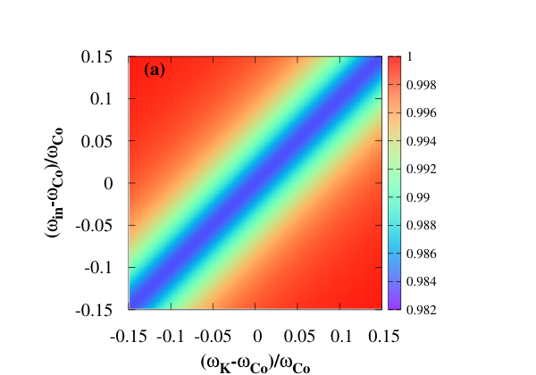
The real parts of S11S_{11} and S12S_{12} are illustrated in Fig. 4 when the magnetizations of nanowire and film are antiparallel.

Refer to caption
Refer to caption
Figure 4: (Color online) Reflection Re⁡(S11)\operatorname{Re}(S_{11}) [(a)] and transmission Re⁡(S12)\operatorname{Re}(S_{12}) [(b)] amplitudes of microwaves, Eq. (A90) between two magnetic nanowires on a magnetic film. ωCo\omega_{\mathrm{Co}} is the Kittel mode frequency Eq. (63) of the cobalt nanowire at a small applied field (Happ=0.05H_{\mathrm{app}}=0.05 T) that fixes an antiparallel magnetizations, ωin\omega_{\mathrm{in}} is the frequency of the input microwaves, and ωK\omega_{\mathrm{K}} is the Kittel mode frequency as a function of an applied field Happ.H_{\mathrm{app}}. The radiative coupling of both nanowires κp/(2​π)=10\kappa_{p}/(2\pi)=10 MHz while other parameter values are listed in the main text.

the interference patterns on the Kittel resonance of cobalt nanowire in Fig. 4(b) reflect the interaction between nanowires and film. The phase factor ei​k​(R1−R2)e^{ik(R_{1}-R_{2})} in Eq. (90) provides peaks and dips when the resonant momentum kk is modulated. These patterns are not caused by spin wave interference in the film since in our model the nanowires cannot reflect spin waves.

V Dipolar non-local spin Seebeck effect

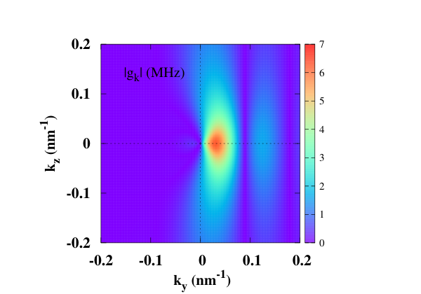
We consider two identical transducers, with a magnetic nanowire at 𝐫2=R2​𝐲^\mathbf{r}_{2}=R_{2}\hat{\mathbf{y}} that detects thermally injected magnons by a nanowire at 𝐫1=R1​𝐲^\mathbf{r}_{1}=R_{1}\hat{\mathbf{y}} with R1<R2R_{1}<R_{2} mediated by the dipolar interaction only. For simplicity, we consider only the Kittel modes in the wires, which is a good approximation at low temperatures at which higher modes are frozen out. The contribution by higher modes with large wave numbers kk is disregarded because the dipolar coupling is exponentially suppressed ∼e−k​x\sim e^{-kx}. The coupling strength |g𝐤||g_{\mathbf{k}}| in Fig. 5 illustrates that magnons with wavelength around half of the nanowire width (π/w=0.045\pi/w=0.045 nm-1) dominate the coupling. Thermal pumping from other than the Kittel mode can be disregarded even at elevated temperatures. Furthermore, the spin current in the film is dominated by spin waves with small momentum and long mean-free paths, so in the following we may disregard the effects of magnon-magnon and magnon-phonon interactions that otherwise render magnon transport phenomena diffuse [9]. The narrow-band thermal injection also favors the inductive detection of the injected spin current pursued here, rather than by the inverse spin Hall effect with heavy metal contacts.

The equation of motions of the Kittel modes in the nanowire and film spin waves in the coupled system read

d​m^Ld​t\displaystyle\frac{d\hat{m}_{L}}{dt} =−i​ωK​m^L−∑qi​gq∗​ei​q​R1​α^q−κ2​m^L−κ​N^L,\displaystyle=-i\omega_{\mathrm{K}}\hat{m}_{L}-\sum_{q}ig_{q}^{\ast}e^{iqR_{1}}\hat{\alpha}_{q}-\frac{\kappa}{2}\hat{m}_{L}-\sqrt{\kappa}\hat{N}_{L},
d​m^Rd​t\displaystyle\frac{d\hat{m}_{R}}{dt} =−i​ωK​m^R−∑qi​gq∗​ei​q​R2​α^q−κ2​m^R−κ​N^R,\displaystyle=-i\omega_{\mathrm{K}}\hat{m}_{R}-\sum_{q}ig_{q}^{\ast}e^{iqR_{2}}\hat{\alpha}_{q}-\frac{\kappa}{2}\hat{m}_{R}-\sqrt{\kappa}\hat{N}_{R},
d​α^qd​t\displaystyle\frac{d\hat{\alpha}_{q}}{dt} =−i​ωq​α^q−i​gq​e−i​q​R1​m^L−i​gq​e−i​q​R2​m^R−κq2​α^q−κq​N^q,\displaystyle=-i\omega_{q}\hat{\alpha}_{q}-ig_{q}e^{-iqR_{1}}\hat{m}_{L}-ig_{q}e^{-iqR_{2}}\hat{m}_{R}-\frac{\kappa_{q}}{2}\hat{\alpha}_{q}-\sqrt{\kappa_{q}}\hat{N}_{q}, (91)

where κ\kappa is caused by the same Gilbert damping in both nanowires, and N^L\hat{N}_{L} and N^R\hat{N}_{R} represent the thermal noise in the left and right nanowires, with ⟨N^η†​(t)​N^η′​(t′)⟩=nη​δ​(t−t′)​δη​η′\langle{\hat{N}_{\eta}^{\dagger}(t)\hat{N}_{\eta^{\prime}}(t^{\prime})}\rangle=n_{\eta}\delta(t-t^{\prime})\delta_{\eta\eta^{\prime}}. Here, η∈{L,R}\eta\in\{L,R\} and nη=1/{exp⁡[ℏ​ωK/(kB​Tη)]−1}n_{\eta}=1/\left\{\exp\left[\hbar\omega_{\mathrm{K}}/(k_{B}T_{\eta})\right]-1\right\} and TRT_{R} is also the film temperature. Integrating out the spin-wave modes in the film, we obtain equations for dissipatively coupled nanowires. In frequency space,

(−i⁡(ω−ωK)+κ2+Γ1+Γ22)​m^L​(ω)+Γ2​ei​q∗​|R2−R1|​m^R​(ω)\displaystyle\left(-i(\omega-\omega_{\mathrm{K}})+\frac{\kappa}{2}+\frac{\Gamma_{1}+\Gamma_{2}}{2}\right)\hat{m}_{L}(\omega)+\Gamma_{2}e^{iq_{\ast}|R_{2}-R_{1}|}\hat{m}_{R}(\omega) =∑qi​gq∗​ei​q​R1​κq​Gq​(ω)​N^q​(ω)−κ​N^L​(ω),\displaystyle=\sum_{q}ig_{q}^{\ast}e^{iqR_{1}}\sqrt{\kappa_{q}}G_{q}(\omega)\hat{N}_{q}(\omega)-\sqrt{\kappa}\hat{N}_{L}(\omega),
(−i⁡(ω−ωK)+κ2+Γ1+Γ22)​m^R​(ω)+Γ1​ei​q∗​|R2−R1|​m^L​(ω)\displaystyle\left(-i(\omega-\omega_{\mathrm{K}})+\frac{\kappa}{2}+\frac{\Gamma_{1}+\Gamma_{2}}{2}\right)\hat{m}_{R}(\omega)+\Gamma_{1}e^{iq_{\ast}|R_{2}-R_{1}|}\hat{m}_{L}(\omega) =∑qi​gq∗​ei​q​R2​κq​Gq​(ω)​N^q​(ω)−κ​N^R​(ω),\displaystyle=\sum_{q}ig_{q}^{\ast}e^{iqR_{2}}\sqrt{\kappa_{q}}G_{q}(\omega)\hat{N}_{q}(\omega)-\sqrt{\kappa}\hat{N}_{R}(\omega), (92)

where Γ1=|gq∗|2/vq∗\Gamma_{1}=|g_{q_{\ast}}|^{2}/v_{q_{\ast}} and Γ2=|g−q∗|2/vq∗\Gamma_{2}=|g_{-q_{\ast}}|^{2}/v_{q_{\ast}} are assumed constant (for the Kittel mode). Here, q∗q_{\ast} is the positive root of ωq∗=ωK\omega_{q_{\ast}}=\omega_{\mathrm{K}} as introduced in the main text.

Refer to caption
Figure 5: (Color online) Momentum dependence of the dipolar coupling strength |g𝐤||g_{\mathbf{k}}| between a nanowire and magnetic film for the dimensions and material parameters used in the main text.

For perfectly chiral coupling with Γ2=0\Gamma_{2}=0 the solutions of Eqs. (92) read

m^L​(ω)\displaystyle\hat{m}_{L}(\omega) =∑qi​gq∗​ei​q​R1​κq​Gq​(ω)​N^q​(ω)−κ​N^L​(ω)−i⁡(ω−ωK)+κ2+Γ12,\displaystyle=\frac{\sum_{q}ig_{q}^{\ast}e^{iqR_{1}}\sqrt{\kappa_{q}}G_{q}(\omega)\hat{N}_{q}(\omega)-\sqrt{\kappa}\hat{N}_{L}(\omega)}{-i(\omega-\omega_{\mathrm{K}})+\frac{\kappa}{2}+\frac{\Gamma_{1}}{2}},
m^R​(ω)\displaystyle\hat{m}_{R}(\omega) =∑qi​gq∗​ei​q​R2​κq​Gq​(ω)​N^q​(ω)−κ​N^R​(ω)−Γ1​eq∗​(R2−R1)​m^L​(ω)−i⁡(ω−ωK)+κ2+Γ12.\displaystyle=\frac{\sum_{q}ig_{q}^{\ast}e^{iqR_{2}}\sqrt{\kappa_{q}}G_{q}(\omega)\hat{N}_{q}(\omega)-\sqrt{\kappa}\hat{N}_{R}(\omega)-\Gamma_{1}e^{q_{\ast}(R_{2}-R_{1})}\hat{m}_{L}(\omega)}{-i(\omega-\omega_{\mathrm{K}})+\frac{\kappa}{2}+\frac{\Gamma_{1}}{2}}. (93)

With m^L,R​(t)=∫e−i​ω​t​m^L,R​(ω)​𝑑ω/(2​π)\hat{m}_{L,R}(t)=\int e^{-i\omega t}\hat{m}_{L,R}(\omega)d\omega/(2\pi), the non-equilibrium occupation of the Kittel modes becomes

ρL\displaystyle\rho_{L} ≡⟨m^L†​(t)​m^L​(t)⟩=nL+∫d​ω2​π​κ(ω−ωK)2+(κ/2+Γ1/2)2​(nq∗−nL),\displaystyle\equiv\langle\hat{m}_{L}^{\dagger}(t)\hat{m}_{L}(t)\rangle=n_{L}+\int\frac{d\omega}{2\pi}\frac{\kappa}{(\omega-\omega_{\mathrm{K}})^{2}+(\kappa/2+\Gamma_{1}/2)^{2}}(n_{q_{\ast}}-n_{L}), (94)
ρR\displaystyle\rho_{R} ≡⟨m^R†​(t)​m^R​(t)⟩=nR+∫d​ω2​π​Γ12​κ[(ω−ωK)2+(κ/2+Γ1/2)2]2​(nL−nq∗),\displaystyle\equiv\langle\hat{m}_{R}^{\dagger}(t)\hat{m}_{R}(t)\rangle=n_{R}+\int\frac{d\omega}{2\pi}\frac{\Gamma_{1}^{2}\kappa}{\left[(\omega-\omega_{\mathrm{K}})^{2}+(\kappa/2+\Gamma_{1}/2)^{2}\right]^{2}}(n_{L}-n_{q_{\ast}}), (95)

where the damping in the film has been disregarded (κq→0)\left(\kappa_{q}\rightarrow 0\right). In the linear regime the non-local thermal injection of magnons into the right transducer by the left one then reads

δ​ρR\displaystyle\delta\rho_{R} ={𝒮CSSE​(TL−TR)0​ when ​TL>TRTL≤TR,\displaystyle=\left\{\begin{array}[c]{c}\mathcal{S}_{\mathrm{CSSE}}(T_{L}-T_{R})\\ 0\end{array}\text{ when }\begin{array}[c]{c}T_{L}>T_{R}\\ T_{L}\leq T_{R}\end{array}\right.,
𝒮CSSE\displaystyle\mathcal{S}_{{}_{\mathrm{CSSE}}} =∫d​ω2​π​Γ12​κ[(ω−ωK)2+(κ/2+Γ1/2)2]2​d​nLd​T|T=(TL+TR)/2.\displaystyle=\int\frac{d\omega}{2\pi}\frac{\Gamma_{1}^{2}\kappa}{\left[(\omega-\omega_{\mathrm{K}})^{2}+(\kappa/2+\Gamma_{1}/2)^{2}\right]^{2}}\left.\frac{dn_{L}}{dT}\right|_{T=\left(T_{L}+T_{R}\right)/2}. (100)

where we defined the chiral (or dipolar) spin Seebeck coefficient 𝒮CSSE.\mathcal{S}_{{}_{\mathrm{CSSE}}}.

The magnon diode effect acts a “Maxwell demon” that rectifies fluctuations in the wire temperature. Of course, in thermal equilibrium all right and left moving magnons are eventually connected by reflection of spin waves at the edges and absorption and re-emission by connected heat baths. The Second Law of thermodynamics is therefore safe, but it might be interesting to search for chirality-induced transient effects.

References

  • [1] T. Yu, C. P. Liu, H. M. Yu, Y. M. Blanter, and G. E. W. Bauer, Phys. Rev. B 99, 134424 (2019).
  • [2] L. Novotny and B. Hecht, Principles of Nano-Optics (Cambridge University Press, Cambridge, England, 2006).
  • [3] L. R. Walker, Phys. Rev. 105, 390 (1957).
  • [4] T. Yu, S. Sharma, Y. M. Blanter, and G. E. W. Bauer, Phys. Rev. B 99, 174402 (2019).
  • [5] G. D. Mahan, Many Particle Physics (Plenum, New York, 1990).
  • [6] E. Šimánek and B. Heinrich, Phys. Rev. B 67, 144418 (2003).
  • [7] C. W. Gardiner and M. J. Collett, Phys. Rev. A 31, 3761 (1985).
  • [8] A. A. Clerk, M. H. Devoret, S. M. Girvin, F. Marquardt, and R. J. Schoelkopf, Rev. Mod. Phys. 82, 1155 (2010).
  • [9] L. J. Cornelissen, J. Liu, R. A. Duine, J. Ben Youssef, and B. J. van Wees, Nat. Phys. 11, 1022 (2015).