Subadditive Load Balancing

Kiyohito Nagano Affiliation: Gunma University Affiliation: k-nagano@gunma-u.ac.jp Akihiro Kishimoto Affiliation: IBM Research, Ireland Email: akihirok@ie.ibm.com

Abstract

Set function optimization is essential in AI and machine learning. We focus on a subadditive set function that generalizes submodularity, and examine the subadditivity of non-submodular functions. We also deal with a minimax subadditive load balancing problem, and present a modularization-minimization algorithm that theoretically guarantees a worst-case approximation factor. In addition, we give a lower bound computation technique for the problem. We apply these methods to the multi-robot routing problem for an empirical performance evaluation.

1 Introduction

A set function is regarded as a discrete function on the vertices of $n$ -dimensional hypercube $\{0,\,1\}^{n}$ . Many combinatorial problems arising in machine learning are reduced to set function optimization. In particular, submodular set functions are a fundamental tool. For example, submodular optimization has been used to perform clustering [31, 29], image segmentation [33, 18] and feature selection [1], and applied to influence maximization [19], sensor placement [14], and text summarization [27].

A set function $f$ is a real-valued function defined on subsets of a finite set $V=\{1,\ldots,\,n\}$ . The domain of $f$ is the power set of $V$ , denoted by $2^{V}=\{S:S\subseteq V\}$ . A set function $f:2^{V}\to\mathbb{R}$ is submodular if $f(S)+f(T)\geq f(S\cup T)+f(S\cap T)$ for all $S,T\subseteq V$ . The submodular set function is known to be a discrete counterpart of the convex function [28]. Similarly to convex functions, submodular functions can be exactly minimized in polynomial time [13, 32, 15]. However, in many practical settings, submodular function minimization becomes a very difficult task even when only one simple additional constraint is introduced [35, 16]. Minimax submodular load balancing (SMLB) is NP-hard. Svitkina and Fleischer [35] presented a sampling-based $O(\sqrt{n\ln n})$ -approximation algorithm. Wei et al. [38] tackled submodular partitioning problems, including minimax SMLB, and presented a majorization-minimization algorithm that ensures a theoretical worst-case approximation factor. Their analysis heavily relies on the curvatures of the submodular functions [37, 17, 34].

A set function $g:2^{V}\to\mathbb{R}$ is subadditive if $g(S)+g(T)\geq g(S\cup T)$ for all $S,T\subseteq V$ . Nonnegative submodularity immediately leads to nonnegative subadditivity whose optimization is important in machine learning [4]. A fractionally subadditive (or XOS) set function, which is a special case of a subadditive set function and a generalization of a submodular set function, is well studied in the context of combinatorial auction [6] and learnability and sketchability of set functions [3, 2, 9]. Despite a simple generalization of submodularity, to the best of our knowledge, little work exists on general subadditive optimization [8]. Therefore, theoretical properties and potential applications of such general subadditive set optimization problems have not been revealed yet.

We, therefore, first examine the subadditivity of fundamental non-submodular functions, including the facility location function [11] and the minimum spanning tree (MST) function. We show that a subadditive set function simplifies computing interpolation of a submodular set function with unknown function values. The interpolation is related to submodular function approximation [10], but our approach is different, since the algorithm of Goemans et al. [10] is not always easy to implement.

We then consider the minimax subadditive load balancing (SALB) problem as an important generalization of SMLB. As a variant of the majorization-minimization algorithm [38] for SMLB, we present the modularization-minimization algorithm that ensures a theoretical worst-case approximation factor. Our analysis reveals the difference and similarity between submodular and subadditive set functions in terms of tractability. While the approximability of SALB implies a tractable aspect of subadditivity, we prove intractability of curvature computation of a subadditive set function. Thus, we introduce a concept of a pseudo-curvature that is relatively tractable. In addition, we present a method for computing a lower bound for SALB in some special cases, including SMLB.

Finally, we discuss that the SALB problem with the MST functions is related to multi-robot routing (MRR) problem with the minimax team objective [23], and perform an empirical evaluation of our approach. Besides, the iterative procedure in the modularization-minimization algorithm attempts to improve a solution found so far. We empirically evaluate the effectiveness of the iterative procedure starting with different initial solutions computed by other existing algorithms for MRR.

2 Subadditive functions and subadditive load balancing

We first give basic definitions, and then define the subadditive load balancing problem.

2.1 Set functions, and subadditive functions

Let $V=[n]:=\{1,\,\ldots,\,n\}$ be a given set of $n$ elements, and $g:2^{V}\to\mathbb{R}$ be a real-valued function defined on all the subset of $V$ . Such a function $g$ is called a set function with a ground set $V$ . A set function $g:2^{V}\to\mathbb{R}$ is called subadditive if $g(S)+g(T)\geq g(S\cup T),\,\forall S,T\subseteq V$ . A set function $g:2^{V}\to\mathbb{R}$ is called submodular if $g(S)+g(T)\geq g(S\cup T)+g(S\cap T),\,\forall S,T\subseteq V$ , and is called modular if $g(S)+g(T)=g(S\cup T)+g(S\cap T),\,\forall S,T\subseteq V$ . A set function is called nonnegative if $0\leq g(S)$ for any $S\subseteq V$ , nondecreasing if $g(S)\leq g(T)$ for any $S,T\subseteq V$ with $S\subseteq T$ , and normalized if $g(\varnothing)=0$ . Trivially, a nonnegative submodular function is a nonnegative subadditive function. Thus subadditivity generalizes submodularity in a simple manner. For an $n$ -dimensional vector $\boldsymbol{z}=(z_{i})_{i\in V}\in\mathbb{R}^{n}$ and $S\subseteq V$ , we denote $z(S)=\sum_{i\in S}z_{i}$ . A set function $z:2^{V}\to\mathbb{R}$ corresponding to the vector $\boldsymbol{z}\in\mathbb{R}^{n}$ is a modular function with $z(\varnothing)=0$ . In the rest of the paper, we basically denote a subadditive set function as $g$ , and a submodular set function as $f$ .

2.2 Examples of subadditive set functions

We examine the subadditivity of some non-submodular functions. The minimum spanning tree function plays an important role in multi-robot routing problems in §5. Another example, a subadditive interpolation of a submodular set function, is given in §2.2.2.

2.2.1 Examples in combinatorial optimization

Minimum spanning tree function.

The minimum spanning tree function is a canonical example of the subadditive set function. Let $r$ be a root node and $V=\{1,\,\ldots,\,n\}$ be a set of other nodes. We are given a distance $d(i,j)\geq 0$ for any $i,\,j\in\widetilde{V}:=\{r\}\cup V$ . Suppose that $d:\widetilde{V}\times\widetilde{V}\to\mathbb{R}$ is symmetric and satisfies triangle inequalities. For any subset $S\subseteq V$ , a minimum spanning tree (MST) w.r.t. $\widetilde{S}:=\{r\}\cup S$ is a spanning tree w.r.t. $\widetilde{S}$ that minimizes the sum of edge distances. For any $S\subseteq V$ , let $MST(S)$ be a sum of edge distances of MST w.r.t. $\widetilde{S}$ . We call $MST:2^{V}\to\mathbb{R}$ a minimum spanning tree function on $V$ with root $r$ .

Lemma 1.

A minimum spanning tree function $MST:2^{V}\to\mathbb{R}$ is nonnegative and subadditive.

The function $MST:2^{V}\to\mathbb{R}$ is not always nondecreasing and/or submodular. For the function $MST$ in Figure 1 (a), $MST(\{1,3\})=10$ and $MST(\{1,2,3\})=9$ . Thus, $MST$ is not nondecreasing. For the function $MST$ in Figure 1 (b), $MST(\{1\})=5$ , $MST(\{1,2\})=MST(\{1,3\})=6$ , and $MST(\{1,2,3\})=9$ . Thus, $MST$ is not submodular.

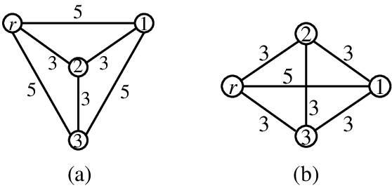
Refer to caption — Figure 1: Minimum spanning tree functions

Let us consider an MST function with nonnegative node weights. Given an MST function $MST:2^{V}\to\mathbb{R}$ and a nonnegative uniform node weight $\beta\geq 0$ , the function $MST^{\beta}:2^{V}\to\mathbb{R}$ defined by

\displaystyle MST^{\beta}(S)=MST(S)+\beta|S|\ (\forall S\subseteq V)

(1)

is also subadditive. The functions $MST$ and $MST^{\beta}$ will be used in the computational experiments on multi-robot routing problems in Section 6.

Facility location function.

The facility location function [11] is another example. Given a finite set $V=\{1,2,\ldots,\,n\}$ of customers and a finite set $F$ of possible locations for the facilities, a certain service is provided by connecting customers to opened facilities. Opening facility $j\in F$ incurs a fixed cost $o_{j}\geq 0$ , and connecting customer $i\in V$ to facility $j\in F$ incurs a fixed cost $c_{ij}\geq 0$ . For any subset $S\subseteq V$ of the customers, let $FL(S)$ be the minimum cost of providing the service only to $S$ . We call $FL:2^{V}\to\mathbb{R}$ a facility location function.

Let us see an example of $FL$ in Figure 2 with $F=\{a,\,b\}$ and $V=\{1,2,3\}$ . We have, e.g., $FL(\{2\})=o_{a}+c_{2a}=2$ , $FL(\{1,\,2\})=o_{a}+c_{1a}+c_{2a}=3$ , and $FL(\{1,\,2,\,3\})=o_{a}+c_{1a}+c_{2a}+o_{b}+c_{3b}=5$ .

Lemma 2.

A facility location function $FL:2^{V}\to\mathbb{R}$ is nondecreasing and subadditive.

As pointed out in [11], $FL:2^{V}\to\mathbb{R}$ is not necessarily submodular. In the case of Figure 2, we have $FL(\{1,2\})+FL(\{2,3\})<FL(\{1,2,3\})+FL(\{2\})$ .

2.2.2 Interpolation of a submodular set function

Let $f:2^{V}\to\mathbb{R}$ be a nondecreasing submodular set function with $f(\varnothing)=0$ . Assume that we have only a part of the function values of $f$ . That is, for a given collection $\mathcal{C}=\{C_{1},\,C_{2},\,\ldots,\,C_{m}\}\subseteq 2^{V}$ , the function values $f(C_{i})=f_{i}$ are known for each $i=1,\ldots,\,m$ and the value $f(S)$ are unknown for any $S\in 2^{V}\setminus\mathcal{C}$ . The objective here is to build a set function $g:2^{V}\to\mathbb{R}$ that approximates $f$ . We introduce a general, simple method to construct a subadditive interpolating set function $g_{\mathcal{C}}$ , which is computationally tractable. We utilize the ideas of the polymatroid [7] and the Lovász extension [28].

In some applications, evaluating function values of $f$ is computationally expensive (see, e.g., [26]). By appropriately setting the collection $\mathcal{C}$ , our interpolation method transforms a complicated submodular optimization problem into a simple subadditive optimization problem.

Lovász extension.

The polymatroid $\mathrm{P}(f)=\{\boldsymbol{z}\in\mathbb{R}^{n}:\mbox{$z(S)\leq f(S)$}\ (\forall S\subseteq V)\}\cap\mathbb{R}_{\geq 0}^{n}$ is a bounded polyhedron, where $\mathbb{R}_{\geq 0}$ is the set of nonnegative real values. The Lovász extension $\widehat{f}:\mathbb{R}_{\geq 0}^{n}\to\mathbb{R}$ is defined by $\widehat{f}(\boldsymbol{x})=\max_{\boldsymbol{z}\in\mathrm{P}(f)}\langle\boldsymbol{x},\boldsymbol{z}\rangle\ \ (\forall\boldsymbol{x}\in\mathbb{R}_{\geq 0}^{n})$ , where $\langle\boldsymbol{x},\boldsymbol{z}\rangle=\sum_{i\in V}x_{i}z_{i}$ . The function $\widehat{f}$ is a natural continuous extension of $f$ since $\widehat{f}(\boldsymbol{I}_{S})=f(S)$ holds, $\forall S\subseteq V$ , where $\boldsymbol{I}_{S}\in\{0,\,1\}^{n}$ is the characteristic vector of $S$ .

Construction of the interpolating function.

For an imitated polymatroid

\mathrm{P}_{\mathcal{C}}(f)=\{\boldsymbol{z}\in\mathbb{R}^{n}:\mbox{$z(C_{i})\leq f(C_{i})$}\ (\forall i=1,\ldots,\,m)\}\cap\mathbb{R}_{\geq 0}^{n},

and an imitated Lovász extension $\widehat{f}_{\mathcal{C}}(\boldsymbol{x})=\max_{\boldsymbol{z}\in\mathrm{P}_{\mathcal{C}}(f)}\langle\boldsymbol{x},\boldsymbol{z}\rangle\ \ (\forall\boldsymbol{x}\in\mathbb{R}_{\geq 0}^{n})$ , we define the set function $g_{\mathcal{C}}:2^{V}\to\mathbb{R}$ as $g_{\mathcal{C}}(S)=\widehat{f}_{\mathcal{C}}(\boldsymbol{I}_{S})\ (\forall S\subseteq V)$ . The following lemma guarantees that $g_{\mathcal{C}}$ is a natural subadditive extension of $f$ and $g_{\mathcal{C}}$ is computationally tractable.

Lemma 3.

The set function $g_{\mathcal{C}}:2^{V}\to\mathbb{R}$ satisfies
(i) $g_{\mathcal{C}}(S)\geq f(S)$ , $\forall S\subseteq V$ , (ii) $g_{\mathcal{C}}(C_{i})=f(C_{i})$ , $\forall i=1,\ldots,\,m$ , (iii) $g_{\mathcal{C}}$ is a nondecreasing subadditive set function, and (iv) the value $g_{\mathcal{C}}(S)$ can be computed in polynomial time in $n$ and $m$ for any given $S\subseteq V$ .

Proof.

Proof of (i). By definition, we have $\mathrm{P}(f)\subseteq\mathrm{P}_{\mathcal{C}}(f)$ . Therefore,

\displaystyle f(S)=\widehat{f}(\boldsymbol{I}_{S})=\max\limits_{\boldsymbol{z}\in\mathrm{P}(f)}\langle\boldsymbol{I}_{S},\boldsymbol{z}\rangle\leq\max\limits_{\boldsymbol{z}\in\mathrm{P}_{\mathcal{C}}(f)}\langle\boldsymbol{I}_{S},\boldsymbol{z}\rangle=\widehat{f}_{\mathcal{C}}(\boldsymbol{I}_{S})=g_{\mathcal{C}}(S),

for all $S\subseteq V$ .

Proof of (ii). By Lemma 3 (i), we have $f(C_{i})\leq g_{\mathcal{C}}(C_{i})$ , $\forall i=1,\ldots,\,m$ . By the definition of $g_{\mathcal{C}}$ and $\mathrm{P}_{\mathcal{C}}(f)$ , we have

g_{\mathcal{C}}(C_{i})=\max\limits_{\boldsymbol{z}\in\mathrm{P}_{\mathcal{C}}(f)}\langle\boldsymbol{I}_{C_{i}},\boldsymbol{z}\rangle=\max\limits_{\boldsymbol{z}\in\mathrm{P}_{\mathcal{C}}(f)}z(C_{i})\leq f(C_{i}),

for all $i=1,\ldots,\,m$ . Thus, we obtain $f(C_{i})=g_{\mathcal{C}}(C_{i})$ , for all $i=1,\ldots,\,m$ .

Proof of (iii). The nondecreasing property of $g_{\mathcal{C}}$ follows from $\mathrm{P}_{\mathcal{C}}(f)\subseteq\mathbb{R}_{\geq 0}^{n}$ . We have $g_{\mathcal{C}}(S\cup T)=\max_{\boldsymbol{z}\in\mathrm{P}_{\mathcal{C}}(f)}\langle\boldsymbol{I}_{S\cup T},\boldsymbol{z}\rangle\leq\max_{\boldsymbol{z}\in\mathrm{P}_{\mathcal{C}}(f)}\langle\boldsymbol{I}_{S}+\boldsymbol{I}_{T},\boldsymbol{z}\rangle\leq\max_{\boldsymbol{z}\in\mathrm{P}_{\mathcal{C}}(f)}\langle\boldsymbol{I}_{S},\boldsymbol{z}\rangle+\max_{\boldsymbol{z}\in\mathrm{P}_{\mathcal{C}}(f)}\langle\boldsymbol{I}_{T},\boldsymbol{z}\rangle=g(S)+g(T)$ , for any $S,\,T\subseteq V$ . Thus, $g_{\mathcal{C}}$ is subadditive.

Proof of (iv). The polyhedron $\mathrm{P}_{\mathcal{C}}(f)$ is bounded and it is determined by $n+m$ linear inequalities. Thus, the linear programming problem $\max\limits_{\boldsymbol{z}\in\mathrm{P}_{\mathcal{C}}(f)}\langle\boldsymbol{I}_{S},\boldsymbol{z}\rangle$ can be solved in polynomial time in $n$ and $m$ . ∎

The function $g_{\mathcal{C}}$ is not necessarily submodular. Consider the case where $V=\{1,2,3\}$ , $f(S)=(7-|S|)|S|\ (\forall S\subseteq V)$ , and $\mathcal{C}=2^{V}\setminus V$ . We have $g_{\mathcal{C}}(\{1\})=6$ , $g_{\mathcal{C}}(\{1,\,2\})=g_{\mathcal{C}}(\{1,\,3\})=10$ , and $g_{\mathcal{C}}(\{1,\,2,\,3\})=15$ . Therefore, $g_{\mathcal{C}}$ is not submodular. Figure 3 illustrates a polymatroid $\mathrm{P}(f)$ and an imitated polymatroid $\mathrm{P}_{\mathcal{C}}(f)$ in the case of this example.

2.3 Subadditive load balancing

We define the submodular load balancing (SMLB) and the subadditive load balancing (SALB) problems. $\mathcal{S}=(S_{1},\,\ldots,\,S_{m})$ is an $m$ -partition of $V=\{1,\ldots,\,n\}$ if $S_{1}\cup\cdots\cup S_{m}=V$ and $S_{j}\cap S_{j^{\prime}}=\varnothing$ for $1\leq j<j^{\prime}\leq m$ (some $S_{j}$ can be empty). Suppose that set functions $f_{1},\,\ldots,\,f_{m}:2^{V}\to\mathbb{R}$ are normalized, nonnegative, and submodular, and set functions $g_{1},\,\ldots,\,g_{m}:2^{V}\to\mathbb{R}$ are normalized, nonnegative, and subadditive. The SMLB problem is defined as

\displaystyle\hskip-5.69054pt\begin{array}[]{ll}\mbox{min}&\max\limits_{j=1,\ldots,\,m}f_{j}(S_{j})\\ \mbox{s.\,t.}&\mathcal{S}=(S_{1},\,\ldots,\,S_{m})\mbox{ is an $m$-partition of }V.\end{array}

We say that SMLB is nondecreasing if $f_{1},\,\ldots,\,f_{m}$ are nondecreasing. Approximation algorithms and heuristics are proposed for the nondecreasing SMLB [35, 38]. On the other hand, we mainly deal with SALB which has not been performed in-depth analysis before. SALB has a slightly different objective function:

\displaystyle\hskip-5.69054pt\begin{array}[]{ll}\mbox{min}&\max\limits_{j=1,\ldots,\,m}g_{j}(S_{j})\\ \mbox{s.\,t.}&\mathcal{S}=(S_{1},\,\ldots,\,S_{m})\mbox{ is an $m$-partition of }V.\end{array}

SALB is nondecreasing for nondecreasing $g_{1},\,\ldots,\,g_{m}$ .

3 Algorithms for SALB

SALB is NP-hard due to the hardness of SMLB. We, therefore, consider some approaches to find approximate solutions of SALB, and begin with the greedy method.

Algorithm

\mbox{{Greedy}}(g_{1},\ldots,g_{m})

0:	Set $S_{j}:=\varnothing$ , $\forall j\in[m]$ , and $U:=V$ .
1:	While $U\neq\varnothing$ do
	Choose $i_{j}\in\arg\min\limits_{i\in R}g_{j}(S_{j}\cup\{i\})$ , $\forall j\in[m]$
	Choose $j^{*}\in\arg\min\limits_{j\in[m]}g_{j}(S_{j}\cup\{i_{j}\})$
	Set $S_{j^{}}:=S_{j^{}}\cup\{i_{j^{}}\}$ and $U:=U\setminus\{i_{j^{}}\}$
2:	Output $\mathcal{S}=(S_{1},\,\ldots,\,S_{m})$ .

Greedy is straightforward but does not empirically yield solutions of good quality (see Section 5). We introduce a nontrivial approach and give new theoretical analyses.

We say that an algorithm $\mathcal{A}$ for the minimization problem (P) achieves an approximation factor of $\gamma\geq 1$ or $\mathcal{A}$ is a $\gamma$ -approximation algorithm if $(OPT\leq)\ APP\leq\gamma\cdot OPT$ is satisfied for any instance of the problem (P), where $OPT$ is the optimal value of the problem and $APP$ is the objective function value of the approximate solution obtained by $\mathcal{A}$ . It is known to be difficult to give a theoretically good approximation algorithm for SALB in a sense. There is no polynomial-time approximation algorithm for the nondecreasing SMLB (and SALB) with an approximation factor of $o(\sqrt{n/\ln n})$ [35]. Therefore, it is important to see the tractability of load balancing problems by using measures different from $n=|V|$ .

As a nontrivial approach to SMLB, Wei et al. [38] proposed a majorization-minimization algorithm and gave a worst-case approximation factor for the nondecreasing submodular case. Its approximation factor depends on the curvatures of the submodular set functions.

We replace $f_{1},\ldots,f_{m}$ in the majorization-minimization algorithm of [38] with $g_{1},\ldots,g_{m}$ , which we call the modularization-minimization algorithm MMin (see §3.1). This replacement leads to the following notable differences and similarities described in this and next sections:

•

Unlike SMLB, a majorizing approximation modular set function for SALB cannot be constructed due to the non-submodular structure.
•

As is the case for SMLB, our analysis uses the curvatures of the subadditive set functions. The worst-case approximation factor of MMin for the nondecreasing SALB in §3.2 is a generalization of the result of [38] for the nondecreasing SMLB.
•

Unlike for a submodular set function, the curvature computation is not easy for a subadditive set function (see §4). Note that the curvature computation is not necessarily required because the algorithm does not use its value.

The approximation guarantee including the curvatures of set functions may be unstable or useless, due to its difficulty of computing the actual value of the approximation factor. In order to resolve this issue, we present a method to compute a lower bound of the optimal solution for some important cases (see §3.3).

3.1 The modularization minimization algorithm

We describe the modularization-minimization algorithm MMin for SALB.

Framework of the algorithm.

MMin iteratively updates the $m$ -partition $\mathcal{S}$ . Given a tentative $m$ -partition $\mathcal{S}^{\prime}=(S^{\prime}_{1},\,\ldots,\,S^{\prime}_{m})$ for SALB, the update operation of each iteration constructs modular approximation function $M_{j}:2^{V}\to\mathbb{R}$ of $g_{j}$ at $S^{\prime}_{j}$ for each $j=1,\ldots,\,m$ , and obtains a modified $m$ -partition $\mathcal{S}^{\prime\prime}=(S_{1}^{\prime\prime},\,\ldots,\,S_{m}^{\prime\prime})$ . $\mathcal{S}^{\prime\prime}$ is an optimal solution to the following modular load balancing (M-LB) problem:

\displaystyle\hskip-5.69054pt\begin{array}[]{ll}\mbox{min}&\max\limits_{j=1,\ldots,\,m}M_{j}(S_{j})\\ \mbox{s.\,t.}&\mathcal{S}=(S_{1},\,\ldots,\,S_{m})\mbox{ is an $m$-partition of }V.\end{array}

Construction of approximation functions.

Given a subadditive set function $g:2^{V}\to\mathbb{R}$ and a subset $S^{\prime}\subseteq V$ , we have to construct a modular approximation set function $M$ of $g$ at $S^{\prime}$ in order to deal with the problem (3.1). If $g$ is submodular, a majorization set function $M$ satisfying $g(S)\leq M(S),\,\forall S$ and $g(S^{\prime})=M(S^{\prime})$ can be constructed in a simple way [38].¹¹ 1 In the submodular case [38], the functions $M^{1}$ and $M^{2}$ defined by, for all $S\subseteq V$ , $M^{1}(S)=g(S^{\prime})+\sum\limits_{i\in S\setminus S^{\prime}}g(i\,|\,S^{\prime})-\sum\limits_{i\in S^{\prime}\setminus S}g(i\,|\,V\setminus\{i\})$ , $M^{2}(S)=g(S^{\prime})+\sum\limits_{i\in S\setminus S^{\prime}}g(i\,|\,\varnothing)-\sum\limits_{i\in S^{\prime}\setminus S}g(i\,|\,S^{\prime}\setminus\{i\})$ are both majorization set functions. These functions are not necessarily majorizing in the subadditive case. In contrast, in the subadditive case, it would be difficult to construct a majorization set function. Thus, for example, we use an intuitively natural modular set function $M$ defined by

M(S)=g(S^{\prime})+\sum\limits_{i\in S\setminus S^{\prime}}g(i\,|\,S^{\prime})-\sum\limits_{i\in S^{\prime}\setminus S}g(i\,|\,S^{\prime}\setminus\{i\})\ \ \ (S\subseteq V),

(8)

where $g(i\,|\,S)=g(S\cup\{i\})-g(S)$ for $S\subseteq V$ and $i\notin S$ . If $g$ is nondecreasing, the marginal cost $g(i\,|\,S)$ is nonnegative for all $S\subseteq V$ and $i\notin S$ .

In computing lower bounds (see § 3.3), we will give an alternative way of constructing the approximation modular set function $M$ which is a minorization set function. The minorization set function $M$ approximating the function $g$ around the subset $S^{\prime}$ satisfies

g(S)\geq M(S),\,\forall S

and

g(S^{\prime})=M(S^{\prime})

We use an approximate minorization set function for some important special cases.

Algorithm description.

MMin is described below.

Algorithm

\mbox{{MMin}}(g_{1},\ldots,g_{m})

0:	Find an initial $m$ -partition $\mathcal{S}^{(0)}=(S_{1}^{(0)},\,\ldots,\,S_{m}^{(0)})$ of $V$ . Set $k:=1$ .
1:	Construct a modular approximation function $M_{j}^{(k)}$ of $g_{j}$ at $S^{(k-1)}_{j}$ , $\forall j\in[m]=\{1,\ldots,\,m\}$ .
2:	Let $\mathcal{S}^{(k)}=(S_{1}^{(k)},\,\ldots,\,S_{m}^{(k)})$ be an $m$ -partition $\mathcal{S}$ that minimizes $\max\limits_{j=1,\ldots,\,m}M_{j}^{(k)}(S_{j})$ .
3:	If $\mathcal{S}^{(k)}=\mathcal{S}^{(k-1)}$
	then output $\mathcal{S}:=\mathcal{S}^{(k)}$ ,
	else set $k:=k+1$ and go to Step 1.

MMin needs to find an initial partition in Step 0, and solve the M-LB problem (3.1) in Step 2. We describe the methods to do so in the following part. In addition, we give a simple approximation bound of MMin for SALB with a mild assumption.

Finding an initial partition.

MMin can start with an arbitrary $m$ -partition of $V$ . In order to obtain an approximation factor for SALB, we consider the M-LB problem

\displaystyle\hskip-5.69054pt\begin{array}[]{l}\mbox{min}\ \ \max\limits_{j=1,\ldots,\,m}M^{(0)}_{j}(S_{j})\\ \mbox{s.\,t.}\ \ \ \,\mathcal{S}=(S_{1},\,\ldots,\,S_{m})\mbox{ is an $m$-partition of }V,\\ \mbox{where }\displaystyle M^{(0)}_{j}(S)=\sum_{i\in S}g_{j}(\{i\})\ (S\subseteq V),\end{array}

and let $\mathcal{S}^{(0)}$ be an optimal (or approximately optimal) partition of problem (3.1).

Solving the modular load balancing.

Each modular set function $M_{j}$ in problem (3.1) is represented as $M_{j}(S)=b_{j}+\sum_{i\in S}c_{ij}\ (S\subseteq V)$ . Therefore, by using a standard MIP (mixed integer programming) formulation technique, problem (3.1) becomes

\displaystyle\begin{array}[]{ll}\mbox{min}&y\\ \mbox{s.\,t.}&\displaystyle\sum_{j\in[m]}x_{ij}=1,\ \forall i\in V,\\ &\displaystyle b_{j}+\sum_{i\in S}c_{ij}x_{ij}\leq y,\ \forall j\in[m],\\ &\displaystyle x_{ij}\in\{0,\,1\},\forall i\in V,\ \forall j\in[m],\ \ y\in\mathbb{R}.\end{array}

An optimal solution to problem (3.1) can be found via MIP solvers such as IBM ILOG CPLEX. An LP-based 2-approximation algorithm of [25] for the unrelated parallel machines scheduling problem can also be used for problem (3.1). However, with the algorithm of Lenstra et al., the approximation factor of 2 can be preserved only when $b_{j}\geq 0\ (\forall j\in[m])$ and $c_{ij}\geq 0\ (\forall i\in V,\,\forall j\in[m])$ .

A simple bound of the algorithm.

For $g:2^{V}\to\mathbb{R}$ , we say that $g$ satisfies a singleton-minimal (SMinimal) property if $g(\{i\})\leq g(S\cup\{i\}),\mbox{ for all }i\in V\mbox{ and }S\subseteq V\setminus\{i\}$ . Any nondecreasing set function and the MST function in §2.2, which is not necessarily nondecreasing, satisfy the SMinimal property. We give a simple approximation bound of MMin for SALB.

Proposition 4.

The algorithm MMin for SALB achieves an approximation factor of $2\cdot(\max_{j\in[m]}|S_{j}^{*}|)$ if each $g_{j}$ satisfies the singleton minimal property, where $\mathcal{S}^{*}=(S_{1}^{*},\,\ldots,\,S_{m}^{*})$ is an optimal partition.

A proof of Proposition 4 uses the definition of the initial partition $\mathcal{S}^{(0)}$ , the following simple relation $M^{(0)}_{j}(S_{j}^{*})=\sum_{i\in S_{j}^{*}}g_{j}(\{i\})\leq|S_{j}^{*}|g_{j}(S_{j}^{*}),$ and the approximation factor of 2 of the algorithm for (3.1). The initial partition of MMin already attains the approximation bound.

3.2 Analysis of the approximation algorithm for nondecreasing SALB

For nondecreasing SALB, the bound of Proposition 4 can be improved by using the curvatures. We give a worst-case approximation factor of the algorithm MMin for the nondecreasing SALB. The following result is a generalization of the result of [38] for the nondecreasing SMLB.

Theorem 5.

The algorithm MMin for the nondecreasing subadditive load balancing achieves an approximation factor of $2\cdot(\max_{j\in[m]}\frac{|S_{j}^{*}|}{1+(|S_{j}^{*}|-1)(1-\kappa_{g}(S_{j}^{*}))})$ , where $\mathcal{S}^{*}=(S_{1}^{*},\,\ldots,\,S_{m}^{*})$ is an optimal partition, and $\kappa_{g_{j}}(S)$ is the curvature of $g_{j}$ at $S\subseteq V$ .

We give a proof of Theorem 5 with the aid of the curvatures of a subadditive set function.

Curvatures and modular approximation functions.

As with the submodular case [37, 17], we consider the curvatures of subadditive functions. Suppose that $g$ is a normalized nondecreasing subadditive set function with $g(\{i\})>0$ for all $i\in V$ . Define the curvature $\kappa_{g}(S)$ of $g$ at $S\subseteq V$ as

\displaystyle\kappa_{g}(S)

\displaystyle=1-\min_{A\subseteq S,\,i\in A}\frac{g(i\,|\,A\setminus\{i\})}{g(\{i\})}.

Denote the total curvature $\kappa_{g}(V)$ by $\kappa_{g}$ .

By the definition of the curvatures, for all $S^{\prime}\subseteq S\subseteq V$ and $i\in S^{\prime}$ , we have $\frac{g(i\,|\,S^{\prime}\setminus\{i\})}{g(\{i\})}\geq 1-\kappa_{g}(S)$ and thus

\displaystyle g(i\,|\,S^{\prime}\setminus\{i\})\geq(1-\kappa_{g}(S))g(\{i\}).

(16)

A set function $\widehat{g}:2^{V}\to\mathbb{R}$ is an $\gamma$ -approximation of $g$ if $g(S)\leq\widehat{g}(S)\leq\gamma g(S)$ for all $S\subseteq V$ . The following lemma evaluates to what extent the modular function

M(S)=\sum_{i\in S}g(\{i\})\ (S\subseteq V)

closely approximates $g$ .

Lemma 6.

If $0<\kappa_{g}<1$ , it holds that

g(S)\leq\sum_{i\in S}g(\{i\})\leq\frac{1}{1-\kappa_{g}}g(S)\ \ (S\subseteq V).

Proof.

The first inequality directly follows from the subadditivity. Suppose $|S|=h$ and $S=\{i_{1},\,\ldots,\,i_{h}\}$ . Let $S_{k}=\{i_{1},\,\ldots,\,i_{k}\}$ for each $k=1,\ldots,\,h$ . Then, by using the inequality (16), we have

g(S)=\sum\limits_{k=1}^{h}g(i_{k}\,|\,S_{k}\setminus\{i_{k}\})\geq(1-\kappa_{g})\sum\limits_{i\in S}g(\{i\}),

which shows the second inequality. ∎

By a more detailed non-uniform analysis, we can obtain a non-uniform version of Lemma 6.

Lemma 7.

For each $S\subseteq V$ , if $0<\kappa_{g}(S)<1$ , it holds that

g(S)\leq\sum_{i\in S}g(\{i\})\leq\frac{|S|}{1+(|S|-1)(1-\kappa_{g}(S))}g(S).

Proof.

Let $S\subseteq V$ be a subset with $|S|=m$ . Fix an element $i\in S$ . Then, we let $S=\{j_{1},\,j_{2},\,\ldots,\,j_{m}\}$ with $j_{1}=i$ , and set $S_{0}=\varnothing$ , $S_{k}=\{j_{1},\,\ldots,\,j_{k}\}\ (k=1,\ldots,\,m)$ . By using the inequality (A1), we have

\displaystyle g(S)-g(\{i\})=\sum^{m}_{k=2}g(j_{k}|S_{k-1})\geq(1-\kappa_{g}(S))\sum_{j\in S\setminus\{i\}}g(\{j\}).

By summing up these inequalities for all $i\in S$ , we have

		$\displaystyle\|S\|g(S)-\sum_{i\in S}g(\{i\})\geq(1-\kappa_{g}(S))(\|S\|-1)\sum_{i\in S}g(\{i\}),$
		$\displaystyle\Longrightarrow\ \|S\|g(S)\geq(1+(1-\kappa_{g}(S))(\|S\|-1))\sum_{i\in S}g(\{i\}),$
		$\displaystyle\Longrightarrow\ \frac{\|S\|}{1+(\|S\|-1)(1-\kappa_{g}(S))}g(S)\geq\sum_{i\in S}g(\{i\}).$

∎

Analysis of the approximation factor.

Here we assume that $g_{1},\,\ldots,\,g_{m}$ are nondecreasing, and $g_{j}(\{i\})>0$ for all $i\in V$ and $j\in[m]$ . In addition, we use a $\gamma_{\mathrm{MLB}}$ -approximation algorithm for problem (3.1) in Step 0 of the algorithm MMin. Notice that the polynomial-time algorithm of [25] for problem (3.1) achieves an approximation factor of 2, that is, $\gamma_{\mathrm{MLB}}=2$ .

To prove Theorem 5, we show that the initial partition $\mathcal{S}^{(0)}$ of the algorithm MMin attains the approximation factor. Thus, it suffices to show the following lemma.

Lemma 8.

Let $\mathcal{S}^{(0)}=(S_{1}^{(0)},\,\ldots,\,S_{m}^{(0)})$ be an optimal partition of problem (3.1), and let $\mathcal{S}^{*}=(S_{1}^{*},\,\ldots,\,S_{m}^{*})$ be an optimal partition of the nondecreasing SALB. Then, $\mathcal{S}^{(0)}$ is a $(\max_{j\in[m]}\frac{|S_{j}^{*}|}{1+(|S_{j}^{*}|-1)(1-\kappa_{g}(S_{j}^{*}))})$ -approximation solution of the nondecreasing SALB.

Proof.

Let $\gamma_{j}^{*}=\frac{|S^{*}_{j}|}{1+(|S^{*}_{j}|-1)(1-\kappa_{g}(S^{*}_{j}))}$ for each $j\in[m]$ . In view of Lemma 7, we have $\sum_{i\in S^{*}_{j}}g_{j}(\{i\})\leq\gamma^{*}_{j}g_{j}(S^{*}_{j})$ for each $j\in[m]$ . Therefore, we have

\displaystyle\max_{j\in[m]}\sum_{i\in S^{*}_{j}}g_{j}(\{i\})\leq(\max_{j\in[m]}\gamma^{*}_{j})\cdot(\max_{j\in[m]}g_{j}(S^{*}_{j})).

(17)

By the subadditivity and the optimality of $\mathcal{S}^{(0)}$ , we have

\displaystyle\max_{j\in[m]}g_{j}(S^{(0)}_{j})\leq\max_{j\in[m]}\sum_{i\in S^{(0)}_{j}}g_{j}(\{i\})\leq\ \max_{j\in[m]}\sum_{i\in S^{*}_{j}}g_{j}(\{i\}).

(18)

Combining (17) and (18), we can see that the partition $\mathcal{S}^{(0)}$ is a $(\max_{j\in[m]}\gamma^{*}_{j})$ -approximation solution of the nondecreasing SALB. ∎

3.3 Lower bound computation

In order to evaluate the quality of the obtained approximation solution, a lower bound of the optimal value of SALB gives an estimate about how close the solution is to the optimal one. We introduce a method to compute a lower bound, which employs the idea behind one iteration of MMin.

3.3.1 A general framework

Given an $m$ -partition $\mathcal{S}^{\prime}=(S^{\prime}_{1},\,\ldots,\,S^{\prime}_{m})$ for SALB, and let $\alpha\geq 1$ . Suppose that, for each $j=1,\ldots,\,m$ , we can construct a modular set function $M_{j}:2^{V}\to\mathbb{R}$ satisfying $\alpha g_{j}(S)\geq M_{j}(S),\,\forall S\subseteq V$ and $g_{j}(S^{\prime}_{j})=M_{j}(S^{\prime}_{j})$ (we call such $M_{j}$ an $\alpha$ -approximate minorization set function of $g_{j}$ at $S^{\prime}_{j}$ ). Then, an optimal solution $\mathcal{S}^{\prime\prime}=(S_{1}^{\prime\prime},\,\ldots,\,S_{m}^{\prime\prime})$ to the M-LB (3.1) with $M_{1},\ldots,\,M_{m}$ provides a lower bound of the optimal value of the SALB. Let $\mathcal{S}^{*}=(S^{*}_{1},\,\ldots,\,S^{*}_{m})$ be an optimal partition to the SALB. For each $j=1,\ldots,\,m$ , the function $M_{j}$ satisfies $M_{j}(S^{*}_{j})\leq\alpha g_{j}(S^{*}_{j})$ . Thus, we have $\max_{j}M_{j}(S^{*}_{j})\leq\alpha\max_{j}g_{j}(S^{*}_{j})$ . By the definition of $\mathcal{S}^{\prime\prime}$ , we have $\max_{j}M_{j}(S^{\prime\prime}_{j})\leq\max_{j}M_{j}(S^{*}_{j})$ . Combining these inequalities, we obtain

\max_{j=1,\,\ldots\,,m}g_{j}(S_{j}^{*})\geq\frac{1}{\alpha}\max_{j=1,\,\ldots\,,m}M_{j}(S_{j}^{\prime\prime}).

Therefore,

\displaystyle LB=\frac{1}{\alpha}\max_{j=1,\,\ldots\,,m}M_{j}(S_{j}^{\prime\prime})

(19)

is a lower bound of the optimal value of the SALB.

The question is how to construct $\alpha$ -approximate minorization set functions with small $\alpha\ (\geq 1)$ . In the remaining part, we deal with the SALB with minimum spanning tree functions (§2.2) and the nondecreasing SMLB.

3.3.2 Lower bound for SALB with MST functions

Given a minimum spanning tree function $MST:2^{V}\to\mathbb{R}$ on the node set $V$ with root $r$ and a subset $S^{\prime}\subseteq V$ , we consider a construction of an $\alpha_{\mathrm{T}}$ -approximate minorization set function $M_{\mathrm{T}}$ of $MST$ at $S^{\prime}$ for some $\alpha_{\mathrm{T}}\geq 1$ . To construct $M_{\mathrm{T}}$ , we use the cost-sharing method for the minimum spanning tree game [5].

Let $\mathcal{T}_{r}$ be a minimum spanning tree w.r.t. $V\cup\{r\}$ . For each $i\in V$ , let $p_{i}$ be the (unique) parent node of $i$ such that $i$ and $p_{i}$ are directly connected on the (unique) path from $i$ to $r$ in $\mathcal{T}_{r}$ . The algorithm of Bird [5] sets the weight $w_{i}$ of $i\in V$ as the distance from $i$ to $p_{i}$ . It holds that $MST(S)\geq\sum_{i\in S}w_{i}\ (\forall S\subseteq V)$ and $\sum_{i\in V}w_{i}=MST(V)$ since the weight vector $\boldsymbol{w}=(w_{i})_{i\in V}\in\mathbb{R}^{n}$ is a core of the minimum spanning tree game. We set $\alpha_{\mathrm{T}}:=MST(S^{\prime})/\sum_{i\in S^{\prime}}w_{i}\ (\geq 1)$ , and define the modular set function $M_{\mathrm{T}}:2^{V}\to\mathbb{R}$ as $M_{\mathrm{T}}(S)=\alpha_{\mathrm{T}}\sum_{i\in S}w_{i}\ (S\subseteq V)$ . Then, we have $\alpha_{\mathrm{T}}MST(S)\geq M_{\mathrm{T}}(S)\ (\forall S\subseteq V)$ and $MST(S^{\prime})=M_{\mathrm{T}}(S^{\prime})$ . Therefore, the function $M_{\mathrm{T}}$ is an $\alpha_{\mathrm{T}}$ -approximate minorization set function of $MST$ at $S^{\prime}$ .

Now we establish a lower bound for the SALB with MST functions $MST_{1},\ldots,\,MST_{m}$ . Given an $m$ -partition $\mathcal{S}^{\prime}=(S^{\prime}_{1},\,\ldots,\,S^{\prime}_{m})$ , we compute weight vector $\boldsymbol{w}^{(j)}$ for each $MST_{j}$ , and we define

\displaystyle\alpha_{\mathrm{max}}=\max_{j=1,\ldots,m}\alpha_{j},

(20)

where $\alpha_{j}=MST_{j}(S^{\prime}_{j})/\sum_{i\in S^{\prime}_{j}}w_{i}^{(j)}$ . Then, we can obtain the lower bound $LB$ in (19) with $\alpha=\alpha_{\mathrm{max}}$ . The quality of $LB$ is empirically evaluated in Section 6.

MST case with uniform node weights.

Given a uniform node weight $\beta\geq 0$ , we can replace $MST_{1},\ldots,\,MST_{m}$ with $MST_{1}^{\beta},\ldots,\,MST_{m}^{\beta}$ , where $MST_{j}^{\beta}(S)=MST_{j}(S)+\beta|S|\ (\forall S\subseteq V)$ . Also in this case, the lower bound for SALB can be computed in the same way as the MST case. We let

\displaystyle\alpha_{\mathrm{max}}^{\beta}=\max_{j=1,\ldots,m}\alpha_{j}^{\beta},

(21)

where $\alpha_{j}^{\beta}=MST_{j}^{\beta}(S^{\prime}_{j})/\sum_{i\in S^{\prime}_{j}}(w_{i}^{(j)}+\beta)$ . Then, we can obtain $LB$ in (19) with $\alpha=\alpha_{\mathrm{max}}^{\beta}$ .

3.3.3 Lower bound for nondecreasing SMLB

Given a normalized nondecreasing submodular set function $f:2^{V}\to\mathbb{R}$ and a subset $S^{\prime}\subseteq V$ , we show a way of constructing an $\alpha$ -approximate minorization set function $M_{f}$ of $f$ at $S^{\prime}$ with $\alpha=1$ .

Let $\boldsymbol{w}=(w_{i})_{i\in V}\in\mathbb{R}^{n}$ be an optimal solution to the linear optimization problem $\max_{\boldsymbol{z}\in\mathrm{P}(f)}\langle\boldsymbol{I}_{S^{\prime}},\boldsymbol{z}\rangle$ over the polymatroid $\mathrm{P}(f)=\{\boldsymbol{z}\in\mathbb{R}^{n}:\mbox{$z(S)\leq f(S)$}\ (\forall S\subseteq V)\}\cap\mathbb{R}_{\geq 0}^{n}$ , where $\boldsymbol{I}_{S^{\prime}}\in\{0,\,1\}^{n}$ is the characteristic vector of $S^{\prime}$ . The vector $\boldsymbol{w}$ can be computed efficiently via the greedy algorithm of Edmonds [7]. Define the modular set function $M_{f}:2^{V}\to\mathbb{R}$ as $M_{f}(S)=\sum_{i\in S}w_{i}\ (S\subseteq V)$ . Then, the definition of the polymatroid implies that $f(S)\geq M_{f}(S),\ \forall S\subseteq V$ , and the correctness of the greedy algorithm of [7] implies that $f(S^{\prime})=M_{f}(S^{\prime})$ . Therefore, the function $M_{f}$ is an exact minorization set function of $f$ at $S^{\prime}$ .

The greedy algorithm of Edmonds.

To make the paper self-contained, we describe the greedy algorithm of Edmonds [7] in detail. For a nonnegative coefficient vector $\boldsymbol{a}=(a_{i})_{i\in V}\in\mathbb{R}^{n}$ , we deal with the linear optimization problem $\max_{\boldsymbol{z}\in\mathrm{P}(f)}\langle\boldsymbol{a},\boldsymbol{z}\rangle$ over the polymatroid $\mathrm{P}(f)$ . Let $L=(v_{1},\,v_{2},\,\ldots,\,v_{n})$ be a total order of $V=\{1,\ldots,\,n\}$ such that $a_{v_{1}}\geq a_{v_{2}}\geq\cdots\geq a_{v_{n}}$ . Define $L(0)=\varnothing$ , $L(1)=\{v_{1}\}$ , $L(2)=\{v_{1},\,v_{2}\}$ , $\ldots$ , and $L(n)=\{v_{1},\,\ldots,\,v_{n}\}$ . The greedy algorithm of Edmonds [7] sets $w_{v_{h}}:=f(L(h))-f(L(h-1))$ for each $v_{h}\in V$ . Then, the vector $\boldsymbol{w}=(w_{i})_{i\in V}\in\mathbb{R}^{n}$ is known to be optimal to $\max_{\boldsymbol{z}\in\mathrm{P}(f)}\langle\boldsymbol{a},\boldsymbol{z}\rangle$ . In addition, it holds that $f(L(h))=w(L(h))$ for each $h=0,1,\,\ldots,\,n$ . In the case of the problem $\max_{\boldsymbol{z}\in\mathrm{P}(f)}\langle\boldsymbol{I}_{S^{\prime}},\boldsymbol{z}\rangle$ , we fix any total order $L=(v_{1},\,\ldots,\,v_{k},\,v_{k+1},\,\ldots,\,v_{n})$ of $V=\{1,\ldots,\,n\}$ such that $S^{\prime}=\{v_{1},\ldots,\,v_{k}\}$ , where $k=|S^{\prime}|$ .

4 Intractability of subadditivity, and countermeasures

Theorem 5 in §3.2 shows a tractable aspect of subadditivity. This section provides some intractable aspects of subadditivity. In addition, as an alternative to the curvature of a subadditive set function, we introduce a concept of a pseudo-curvature.

4.1 Intractability of subadditivity

Unconstrained minimization.

For submodular set function $f:2^{V}\to\mathbb{R}$ with $V=[n]$ , the unconstrained minimization problem $\min_{S\subseteq V}f(S)$ is exactly solved in polynomial time [13, 32, 15]. On the other hand, we prove that the unconstrained subadditive minimization is not tractable. We derive the intractability from the NP-hardness of the prize-collecting Steiner tree (PCST) problem of Goemans and Williamson [12].

Theorem 9.

For subadditive set function $g:2^{V}\to\mathbb{R}$ , the problem $\min_{S\subseteq V}g(S)$ is NP-hard.

Proof.

Given an $n$ -dimensional nonnegative prize vector $\boldsymbol{p}=(p_{i})_{i\in V}\in\mathbb{R}^{n}$ and a minimum spanning tree function $MST:2^{V}\to\mathbb{R}$ defined in §2.2, let us consider a set function $PCST:2^{V}\to\mathbb{R}$ defined by

\displaystyle PCST(S)=MST(S)+p(V\setminus S)\ \ (S\subseteq V).

The PCST of Goemans and Williamson [12], which is NP-hard, coincides with the minimization problem $\min_{S\subseteq V}PCST(S)$ . In addition, owing to the subadditivity of $MST(S)$ and the nonnegative modularity of $p(V\setminus S)$ , $PCST$ is subadditive. Therefore, the PCST is a special case of the unconstrained subadditive minimization problem. Thus, the subadditive function minimization is NP-hard. ∎

Curvature computation.

For a submodular set function, it is easy to calculate curvatures [37, 17]. On the other hand, we prove that the curvature computation is not a trivial task in the subadditive case. We derive the intractability from the NP-hardness of the maximization problem of a nondecreasing submodular set function, which is a well-known NP-hard problem.

Theorem 10.

For a subadditive set function $g:2^{V}\to\mathbb{R}$ and $S\subseteq V$ , the computation of curvature $\kappa_{g}(S)=1-\min\limits_{A\subseteq S,\,i\in A}\frac{g(A)-g(A\setminus\{i\})}{g(\{i\})}$ is NP-hard.

Proof.

Let $i^{*}=n$ be a fixed element of $V=[n]$ , and let $U=V\setminus\{i^{*}\}=[n-1]$ . In view of the definition of the curvature, it suffices to show the NP-hardness of the minimization problem $\min_{A\subseteq U}(g(A\cup\{i^{*}\})-g(A))$ . To prove the NP-hardness, we construct a subadditive function $g$ using a nonnegative submodular function.

Let $\widetilde{f}:2^{U}\to\mathbb{R}$ be a general nonnegative submodular function. Then, we define a set function $g:2^{V}\to\mathbb{R}$ with the ground set $V=U\cup\{i^{*}\}$ as

\displaystyle g(A)=\left\{\begin{array}[]{ll}\widetilde{f}(A)&(A\subseteq U=V\setminus\{i^{*}\}),\\ 0&(i^{*}\in A\subseteq V).\end{array}\right.

Trivially, $g$ is nonnegative. Moreover, we can see that $g$ always satisfies the subadditive inequality $g(A)+g(B)\geq g(A\cup B)$ for all $A,\,B\subseteq V$ . ((i) If $i^{*}\in A\cup B$ , we have $g(A\cup B)=0\leq g(A)+g(B)$ . (ii) If $i^{*}\notin A\cup B$ , the nonnegative submodularity of $\widetilde{f}$ gives the subadditive inequality of $g$ .) Now, the minimization problem $\min_{A\subseteq U}(g(A\cup\{i^{*}\})-g(A))$ is equivalent to the submodular maximization problem $\max_{A\subseteq U}\widetilde{f}(A)$ , which is known to be NP-hard. Therefore, the curvature computation is NP-hard for a subadditive set function. ∎

4.2 Pseudo-curvatures

As a countermeasure to the difficulty of the curvature calculation of a subadditive set fuction (Theorem 10), we introduce a concept of a pseudo-curvature.

Given a nonnegative subadditive set function $g:2^{V}\to\mathbb{R}$ , we suppose that $g$ can be decomposed as follows:

g(S)=g_{+}(S)+f_{+}(S)\ (\forall S\subseteq V),

where $g_{+}$ is subadditive and approximately or exactly nondecreasing, and $f_{+}$ is nonnegative and submodular (or nonnegative and modular). If $g_{+}$ is exactly nondecreasing, the total curvature $\kappa_{g}$ of $g$ can be bounded as follows:

	$\displaystyle\kappa_{g}$	$\displaystyle=\mbox{$1-\min\limits_{A\subseteq V,\,i\in A}\frac{g_{+}(i\,\|\,A\setminus\{i\})+f_{+}(i\,\|\,A\setminus\{i\})}{g(\{i\})}$}$
		$\displaystyle\leq\mbox{$1-\min\limits_{A\subseteq V,\,i\in A}\frac{f_{+}(i\,\|\,A\setminus\{i\})}{g(\{i\})}$}$
		$\displaystyle=\mbox{$1-\min\limits_{i\in V}\frac{f_{+}(i\,\|\,V\setminus\{i\})}{g(\{i\})}$}.$

An appropriate decomposition $g=g_{+}+f_{+}$ would make the value $\widehat{\kappa}_{g}:=1-\min_{i\in V}\frac{f_{+}(V)-f_{+}(V\setminus\{i\})}{g(\{i\})}$ a reasonable alternative to the total curvature $\kappa_{g}$ even if $g_{+}$ is approximately nondecreasing. We call $\widehat{\kappa}_{g}$ a pseudo-curvature.

Let us consider the case where $g(S)=MST^{\beta}(S)=MST(S)+\beta|S|$ defined in (1). The function $MST$ is nonnegative and subadditive (Lemma 1). Although $MST$ is not strictly nondecreasing, it can be regarded as an approximately nondecreasing set function. In addition, the term of $\beta|S|(=f_{+}(S))$ is modular and nonnegative. Therefore, the pseudo-curvature $\widehat{\kappa}_{MST^{\beta}}$ is given by

	$\displaystyle\widehat{\kappa}_{MST^{\beta}}$	$\displaystyle=1-\mbox{$\min\limits_{i\in V}\frac{\beta\|V\|-\beta\|V\setminus\{i\}\|}{MST^{\beta}(\{i\})}$}$
		$\displaystyle=1-\mbox{$\min\limits_{i\in V}\frac{\beta}{d(r,i)+\beta}$}.$		(22)

The relationship between the performance of the proposed algorithm and the pseudo-curvature will be discussed in Section 6.

5 Application to multi-robot routing

This section explains an application of the subadditive load balancing (SALB) to the multi-robot routing (MRR) problem with the minimax team objective.

For a set of robots $\mathcal{R}=\{r_{1},\ldots,r_{m}\}$ , a set of targets, $\mathcal{T}=\{t_{1},\ldots,t_{n}\}$ , and any $i,\,j\in\mathcal{R}\cup\mathcal{T}$ , a nonnegative cost (distance) $d(i,j)\geq 0$ is determined. The cost function $d:(\mathcal{R}\cup\mathcal{T})\times(\mathcal{R}\cup\mathcal{T})\to\mathbb{R}$ is symmetric and satisfies triangle inequalities. We consider an allocation of targets to robots. Let $S_{j}\subseteq\mathcal{T}$ be a target subset allocated to robot $r_{j}\in\mathcal{R}$ . MRR with the minimax team objective asks for finding an $m$ -partition $\mathcal{S}=(S_{1},\,\ldots,\,S_{m})$ of $\mathcal{T}$ and a path $P_{j}$ for each robot $r_{j}\in\mathcal{R}$ that visits all targets in $S_{j}$ so that a team objective is optimized [23] as follows:

	$\displaystyle\mathrm{Minimax:}\ \$	$\displaystyle\min_{\mathcal{S}}\max_{j\in\mathcal{R}}RPC_{j}(S_{j})$
		$\displaystyle\ \mbox{or }\ \min_{\mathcal{S}}\max_{j\in\mathcal{R}}RTC_{j}(S_{j}),$

where $RPC_{j}(S_{j})$ is the minimum value of the robot path cost (RPC) for robot $r_{j}\in\mathcal{R}$ to visit all targets in $S_{j}$ , and $RTC_{j}(S_{j})$ is the minimum value of the robot tree cost (RTC) for robot $r_{j}\in\mathcal{R}$ , i.e., $RTC_{j}(S_{j})$ is the sum of edge cost of an MST on $\{r_{j}\}\cup S_{j}$ . The RPC is intractable due to the NP-hardness of the traveling salesperson problem, but the RTC is tractable. An MST on $\{r_{j}\}\cup S_{j}$ can be converted to a robot path on $\{r_{j}\}\cup S_{j}$ whose cost is within $1.5\cdot RPC_{j}(S_{j})$ (see, e.g., [36]).

Approximation algorithms especially based on sequential single-item auctions have been extensively studied to solve MRR [21]. Our approach based on SALB provides a new, different way of tackling MRR with the minimax team objective. Because $RTC_{j}(S_{j})$ is an MST function (see §2.2), it is an example of the subadditive set function. In addition, the lower bound analysis of §3.3 can be utilized.

We can also deal with the processing time of targets. Let $\beta\geq 0$ be a (uniform) waiting time it takes each robot to process each target. Then, each $RTC_{j}$ becomes an MST function with a uniform node weight, which is defined in (1). Furthermore, even in this case, we can use the lower bound analysis of §3.3, and the pseudo-curvatures can be computed in view of (22).

6 Experimental results

Table 1: Quality of RTC for MST and MMin

Target	MST		Initial		MMin		MMin + MST		Lower bound
size	RTC	Time (s)	RTC	Time (s)	RTC	Time (s)	RTC	Time (s)	RTC	Time (s)	$\alpha_{\mathrm{max}}$
50	4220	0.00024	4735	0.78	3827	1.32	3628	0.52	1914	193.26	1.66
100	5484	0.0016	6626	15.50	5111	16.43	4797	0.73	3064	13.32	1.42
120	5886	0.0042	7147	81.48	5474	82.54	5189	0.87	3422	7.17	1.38

We performed empirical evaluation in the MRR domain on a machine with four Intel CPU cores (i5-6300U at 2.40GHz, only one core in use) and 7.4 GB of RAM. Our C++ implementation of the modularization-minimization algorithm denoted by MMin, runs IBM ILOG CPLEX to optimally solve each LP problem generated by MMin. MMin terminates if the value of the LP problem in the current iteration agrees with one in a previous iteration. We also implemented the following well-known MRR algorithms:

$\bullet$	MST [23] is a standard algorithm presented in Algorithm Greedy, which is very similar to GreedMin of Wei et al. [38]. When MST calculates the RPC value, each robot’s MST needs to be converted to a path. We used short-cutting [24], commonly used in MRR [23, 20].
$\bullet$	Path [23] is a standard auction algorithm in the literature [21]. Starting with a null path, each robot greedily extends its path with the insertion heuristic [24]. The robot with the smallest RPC wins an unassigned target in each round. This step is repeated until all targets are assigned.

In calculating the RPC value for MMin, our approach generated a path based on the insertion heuristic with a partition calculated by MMin (i.e., the assignment optimized for RTC). We prepared a road map of the Hakodate area in Japan and precomputed distances between locations. That is, the distance was immediately retrieved when necessary. This is a common experimental setting for MRR, e.g., [22, 39]. In practice, when the map only contains a small city, all distance information fits into memory e.g., [30]. The precomputed distances correspond to driving times in second. We always set the robot size to five, but prepared three cases for the target size (50, 100 and 120). Each case consisted of 100 instances by randomly placing agents and targets.

Table 2: Quality of RTC for MST and MMin with 120 targets and 5 robots.

Waiting	MST		Initial		MMin		MMin + MST		Pseudo
Time	RTC	Time (s)	RTC	Time (s)	RTC	Time (s)	RTC	Time (s)	Curvature
10	6095	0.0032	7195	70.77	5617	72.11	5393	1.17	0.997
30	6656	0.0027	7668	21.33	6100	22.80	5907	1.35	0.991
60	7476	0.0025	8314	32.68	6790	34.49	6661	1.77	0.983

Table 3: Quality of RPC for each method

Target size	MST	Path	MMin	MMin + MST
50	5233	4979	5011	4767
100	7255	6900	7182	6827
120	7756	7484	7870	7446

Table 1 shows average RTC values and average runtimes. We excluded Path here, since it does not optimize for RTC. The values in “Initial” indicate the RTC values and runtimes for finding initial $m$ -partitions of MMin. The iterative procedure of MMin is regarded as a step to further refine an initial solution. Therefore, another initial solution can be passed to this iteration, although the worst-case theoretical analysis of the solution quality remains future work. We prepared MMin + MST that performs the MMin iterations but starts with an initial $m$ -partition calculated by MST.

MMin generated 9%, 7%, and 7% smaller RTC values than MST with 50, 100 and 120 targets, respectively. While the RTC values of the initial partitions generated by solving the first LP problems were inferior to those of MST, MMin’s iterative steps successfully improved the initial partitions.

In case of 50 targets, MMin performed 19 iterations on average, ranging between 4 and 76 iterations. In case of 120 targets, the number of iterations was 22 on average, ranging between 6 and 92 iterations. Among these iterations, MMin typically spent 59-99 % of the runtime in finding an initial partition. The formulation of the initial LP problem is slightly different from those in the remaining iterations, which we hypothesize as a cause of the difficulty. Finding the initial partition tended to be harder with a larger target size. In solving the most difficult instance with 50 targets, MMin needed 13.27 seconds to find an initial partition and only 0.75 seconds for the remaining iterations. There was one instance with 120 targets which took MMin 7317 seconds to find an initial partition.

MMin + MST performed best in terms of the RTC quality and runtime. It bypassed the significant overhead of the initial partition computation, and started with a better initial RTC value than standard MMin. This indicates that such a hybrid approach is important in practice. The results shown in [23] seem to indicate that the worst-case solutions of auction-based algorithms are bounded by $O(m)$ . However, MMin is a centralized approach, and a question remains open as future work regarding whether MMin + MST theoretically guarantees a better approximation factor in general or not.

We calculated an average lower bound and $\alpha_{\mathrm{max}}$ defined in (20) for each target size (see Table 1) with the method presented in §3.3 and with the partition returned by MMin + MST. These lower bounds indicate that on average the approximation factors of MMin + MST were empirically better than 1.90, and 1.57 and 1.52 for 50, 100, and 120 targets, respectively. We observed that there were many instances whose larger lower bounds were returned if different partitions (e.g., a partition that is better than in the previous iterations) were used for the lower bound computation. Therefore, in fact, MMin + MST must yield solutions closer to optimal than those potential approximation factors.

The average runtime to compute a lower bound increased when the target size decreased, which was counter-intuitive. However, the potential approximation factors and the $\alpha_{\mathrm{max}}$ values increased with a decrease of the target size. Therefore, we hypothesize that the LP problem for lower bound calculation tends to be more difficult if the lower bound is farther than the optimal solution.

Next, let us see the performance of the algorithms with waiting time $\beta\geq 0$ . Table 3 shows the cases where waiting times are varied from 10–60 seconds with 5 robots and 120 targets. The waiting time corresponds to the time necessary for a robot to collect and drop off a target. We observed similar tendencies, even when waiting times were introduced. MMin returns better RTC values than MST, but suffers from the computational overhead for solving the initial LP problem. MMin+MST bypasses this overhead as well as yields the best RTC values. The values of the pseudo-curvature $\widehat{\kappa}_{MST^{\beta}}$ determined in (22) close to 1 indicate a difficulty of performing theoretical analysis, even with waiting times. When the waiting time $\beta$ was set to 60, the value of $\alpha^{\beta}_{\mathrm{max}}$ defined in (21) was 1.32, which was smaller than that without waiting time (i.e., $\alpha_{\mathrm{max}}=1.38$ as shown in Table 1, and the pseudo-curvature is 1). This result implies the relative tractability of the problem with $\beta=60$ .

Table 3 shows RPC values of each method. Since our approach does not optimize for the RPC, algorithms that obtain better RTC values do not always yield better RPC values in theory. However, in practice, MMin + MST performed best of all methods.

While Path and MST guarantee the same theoretical approximation factor to optimal RPC values in MRR, there has been consensus that Path tends to perform better than MST [23], as is the case in our experiment. However, our results are important in the sense that they indicate that approaches that optimize solutions for the RTC metric (i.e., the MST function) and then convert to a path have a potential to become a better approach than Path, which would open up further research opportunities.

7 Concluding remarks

We presented the modularization-minimization algorithm for the subadditive load balancing, and gave an approximation guarantee for the nondecreasing subadditive case. We also presented a lower bound computation technique for the problem. In addition, we evaluated the performance of our algorithm in the multi-robot routing domain. The application of subadditive optimization to AI are new, and subadditive approaches may open up a new field of AI and machine learning. An example of future work is to elucidate the theoretical and empirical behaviors of the modularization-minimization algorithm with respect to the initial solutions. Our results about giving the MMin iteration procedure an initial partition calculated by an MST-based greedy algorithm show the importance of the choice of the initial solutions. On other other hand, the question whether or not the iterative procedure currently contributes to improving the worst-case approximation factor remains unanswered.

References

[1] F. Bach. Learning with submodular functions: A convex optimization perspective. Foundations and Trends in Machine Learning, 6(2–3):145–373, 2013.
[2] A. Badanidiyuru, S. Dobzinski, H. Fu, R. Kleinberg, N. Nisan, and T. Roughgarden. Sketching valuation functions. In SODA ’12, pages 1025–1035, 2012.
[3] M.-F. Balcan and N. Harvey. Submodular functions: Learnability, structure, and optimization. SIAM Journal on Computing, 47:703–754, 2018.
[4] A. A. Bian, J. M. Buhmann, A. Krause, and S. Tschiatschek. Guarantees for greedy maximization of non-submodular functions with applications. In ICML, pages 498–507, 2017.
[5] C. G. Bird. On cost allocation for a spanning tree: A game theoretic approach. Networks, 6:335–350, 1976.
[6] S. Dobzinski, N. Nisan, and M. Schapira. Approximation algorithms for combinatorial auctions with complement-free bidders. Mathematics of Operations Research, 35:1–13, 2010.
[7] J. Edmonds. Submodular functions, matroids, and certain polyhedra. In Combinatorial Structures and Their Applications (R. Guy, H. Hanani, N. Sauer, J. Schonheim, eds.), pages 69–87. Gordon and Breach, 1970.
[8] U. Feige. On maximizing welfare when utility functions are subadditive. SIAM J. Comput., 39(1):122–142, 2009.
[9] V. Feldman and J. Vondrák. Optimal bounds on approximation of submodular and xos functions by juntas. SIAM Journal on Computing, 45:1129–1170, 2016.
[10] M. X. Goemans, N. Harvey, S. Iwata, and V. Mirrokni. Approximating submodular functions everywhere. In SODA ’09, pages 535–544, 2009.
[11] M. X. Goemans and M. Skutella. Cooperative facility location games. Journal of Algorithms, 50:194–214, 2004.
[12] M. X. Goemans and D. P. Williamson. A general approximation technique for constrained forest problems. SIAM Journal on Computing, 24:296–317, 1995.
[13] M. Grötschel, L. Lovász, and A. Schrijver. Geometric Algorithms and Combinatorial Optimization. Springer, 1988.
[14] C. Guestrin, A. Krause, and A.P. Singh. Near-optimal sensor placements in gaussian processes. In ICML, pages 265–272, 2005.
[15] S. Iwata, L. Fleischer, and S. Fujishige. A combinatorial strongly polynomial algorithm for minimizing submodular functions. Journal of the ACM, 48:761–777, 2001.
[16] S. Iwata and K. Nagano. Submodular function minimization under covering constraints. In FOCS’09, pages 671–680, 2009.
[17] R. K. Iyer, S. Jegelka, and J. Bilmes. Curvature and optimal algorithms for learning and minimizing submodular functions. In NIPS, pages 2742–2750, 2013.
[18] S. Jegelka and J. Bilmes. Submodularity beyond submodular energies: coupling edges in graph cuts. In CVPR’11, pages 1897–1904, 2011.
[19] D. Kempe, J. Kleinberg, and E. Tardos. Maximizing the spread of influence through a social network. In KDD’03, pages 137–146, 2003.
[20] A. Kishimoto and N. Sturtevant. Optimized algorithms for multi-agent routing. In AAMAS, pages 1585–1588, 2008.
[21] S. Koenig, P. Keskinocak, and C. Tovey. Progress on agent coordination with cooperative auctions. In AAAI, pages 1713–1717, 2010.
[22] S. Koenig, C. Tovey, X. Zheng, and I. Sungur. Sequential bundle-bid single-sale auction algorithms for decentralized control. In IJCAI, pages 1359–1365, 2007.
[23] M. G. Lagoudakis, E. Markakis, D. Kempe, P. Keskinocak, A. Kleywegt, S. Koenig, C. Tovey, A. Meyerson, and S. Jain. Auction-based multi-robot routing. In Proc. of Robotics: Science and Systems, 2005.
[24] E. L. Lawler, J. K. Lenstra, A. H. G. R. Kan, and D. B. Shmoys. The Traveling Salesman Problem: A Guided Tour of Combinatorial Optimization. Wiley Series in Discrete Mathematics and Optimization, 1985.
[25] J. K. Lenstra, D. B. Shmoys, and E. Tardos. Approximation algorithms for scheduling unrelated parallel machines. Math. Program., 46:259–271, 1990.
[26] J. Leskovec, A. Krause, C. Guestrin, C. Faloutsos, J. VanBriesen, and N. Glance. Cost-effective outbreak detection in networks. In KDD ’07, pages 420–429, 2007.
[27] H. Lin and J. Bilmes. Multi-document summarization via budgeted maximization of submodular functions. In HLT’10, pages 912–920, 2010.
[28] L. Lovász. Submodular functions and convexity. In A. Bachem, M. Grötschel, and B. Korte, editors, Mathematical Programming — The State of the Art, pages 235–257. Springer-Verlag, 1983.
[29] K. Nagano, Y. Kawahara, and S. Iwata. Minimum average cost clustering. In NIPS, pages 1759–1767, 2010.
[30] H. Nakashima, S. Sano, K. Hirata, Y. Shiraishi, H. Matsubara, R. Kanamori, H. Koshiba, and Itsuki Noda. One cycle of smart access vehicle service development. In Proc. of the 2nd International Conf. on Serviceology, pages 152–157, 2014.
[31] M. Narasimhan, N. Jojic, and J. Bilmes. Q-clustering. In NIPS, pages 979–986, 2005.
[32] A. Schrijver. A combinatorial algorithm minimizing submodular functions in strongly polynomial time. Journal of Combinatorial Theory (B), 80:346–355, 2000.
[33] P. Stobbe and A. Krause. Efficient minimization of decomposable submodular functions. In NIPS, pages 2208–2216, 2010.
[34] M. Sviridenko, J. Vondrák, and J. Ward. Optimal approximation for submodular and supermodular optimization with bounded curvature. In SODA’15, pages 1134–1148, 2015.
[35] Z. Svitkina and L. Fleischer. Submodular approximation: sampling-based algorithms and lower bounds. In FOCS’08, pages 697–706, 2008.
[36] Vijay V. Vazirani. Approximation Algorithms. Springer-Verlag New York, Inc., 2001.
[37] Jan Vondrak. Submodularity and curvature: the optimal algorithm. In RIMS Kokyuroku Bessatsu, volume B23, volume B23, pages 253–266, 2010.
[38] K. Wei, R. K. Iyer, S. Wang, W. Bai, and J. A. Bilmes. Mixed robust/average submodular partitioning: Fast algorithms, guarantees, and applications. In NIPS, pages 2233–2241, 2015.
[39] X. Zheng, S. Koenig, and C. Tovey. Improving sequential single-item auctions. In IROS, pages 2238– 2244, 2006.

Supplementary Material

A.1 Proofs of Subadditivity

We show the subadditivity of the minimum spanning tree function $MST$ and the facility location function $FL$ defined in §2.2.

A.1.1 Subadditivity of minimum spanning tree function

In the field of game theory, the subadditivity of the minimum spanning tree function is recognized in relation to the minimum spanning tree game (Bird [5]). Here, we describe the proof of Lemma 1 to make the paper self-contained.

Lemma 1 (§2.2.1). A minimum spanning tree function $MST:2^{V}\to\mathbb{R}$ is nonnegative and subadditive.

Proof.

By definition, nonnegativity is trivial. For subsets $S,T\subseteq V$ , let $E_{S}$ be the edge set of MST w.r.t. $\widetilde{S}$ and let $E_{T}$ be the edge set of MST w.r.t. $\widetilde{T}$ . The graph $(S\cup T\cup\{r\},\,E_{S}\cup E_{T})$ with a node set $S\cup T\cup\{r\}$ and an edge set $E_{S}\cup E_{T}$ are connected. Thus we have $MST(S)+MST(T)=\sum_{e\in E_{S}\cup E_{T}}d(e)\geq MST(S\cup T),$ which shows the subadditivity of $MST$ . ∎

A.1.2 Subadditivity of facility location function

We show the subadditivity of the facility location function.

Lemma 2 (§2.2.1). A facility location function $FL:2^{V}\to\mathbb{R}$ is nondecreasing and subadditive.

Proof.

We are given a set $V=\{1,\ldots,\,n\}$ of customers and a finite set $F$ of possible locations for the facilities with opening costs $o_{j}\geq 0$ $(\forall j\in F)$ and connecting costs $c_{ij}\geq 0$ $(\forall(i,\,j)\in V\times F)$ . For each edge subset $\mathcal{E}\subseteq V\times F$ , let $N(\mathcal{E})$ be a set of all endpoints of $\mathcal{E}$ , and we denote $V(\mathcal{E}):=V\cap N(\mathcal{E})$ and $F(\mathcal{E}):=F\cap N(\mathcal{E})$ .

For $S\subseteq V$ , $F^{\prime}\subseteq F$ , and $\mathcal{E}\subseteq V\times F$ , we say that a triple $\mathcal{T}=(S,\,F^{\prime},\mathcal{E})$ is feasible if $S\subseteq V(\mathcal{E})$ and $F(\mathcal{E})\subseteq F^{\prime}$ . For any feasible triple $\mathcal{T}=(S,\,F^{\prime},\mathcal{E})$ , we define $\mathrm{cost}(\mathcal{T}):=\sum_{j\in F^{\prime}}o_{j}+\sum_{(i,j)\in\mathcal{E}}c_{ij}$ , and we have $FL(S)\leq\mathrm{cost}(\mathcal{T})$ . In addition, for each $S\subseteq V$ , there exists a feasible triple $\mathcal{T}^{*}=(S,\,F^{*},\mathcal{E}^{*})$ such that $FL(S)=\mathrm{cost}(\mathcal{T}^{*})$ .

Suppose that $S^{\prime}\subseteq S\subseteq V$ . Let $\mathcal{T}^{*}=(S,\,F^{*},\mathcal{E}^{*})$ be a feasible triple satisfying $FL(S)=\mathrm{cost}(\mathcal{T}^{*})$ . Then, $\mathcal{T}^{\prime}=(S^{\prime},\,F^{*},\mathcal{E}^{*})$ is also a feasible triple. Therefore, $FL(S^{\prime})\leq\mathrm{cost}(\mathcal{T}^{\prime})=\mathrm{cost}(\mathcal{T}^{*})=FL(S)$ , which implies the nondecreasing property of $FL$ .

Suppose that $S_{1},S_{2}\subseteq V$ . For each $k\in\{1,2\}$ , let $\mathcal{T}^{*}_{k}=(S_{k},F^{*}_{k},\mathcal{E}^{*}_{k})$ be a feasible triple such that $FL(S_{k})=\mathrm{cost}(\mathcal{T}^{*}_{k})$ . Since $\mathcal{T}^{*}_{1}\cup\mathcal{T}^{*}_{2}=(S_{1}\cup S_{2},F^{*}_{1}\cup F^{*}_{2},\mathcal{E}^{*}_{1}\cup\mathcal{E}^{*}_{2})$ is feasible, we have $FL(S_{1}\cup S_{2})\leq\mathrm{cost}(\mathcal{T}^{*}_{1}\cup\mathcal{T}^{*}_{2})\leq\mathrm{cost}(\mathcal{T}^{*}_{1})+\mathrm{cost}(\mathcal{T}^{*}_{2})=FL(S_{1})+FL(S_{2})$ , which implies the subadditivity of $FL$ . ∎

A.2 Supplementary Explanation for §3.1

Let us see that it would be difficult to construct a majorization set function in the subadditive case.

Given a subadditive set function $g:2^{V}\to\mathbb{R}$ and a subset $S^{\prime}\subseteq V$ , define the functions $M^{1}$ and $M^{2}$ as, for all $S\subseteq V$ ,

	$\displaystyle M^{1}(S)=g(S^{\prime})$	$+\sum\limits_{i\in S\setminus S^{\prime}}g(i\,\|\,S^{\prime})$ $-\sum\limits_{i\in S^{\prime}\setminus S}g(i\,\|\,V\setminus\{i\}),$
	$\displaystyle M^{2}(S)=g(S^{\prime})$	$\displaystyle\mbox{$+\sum\limits_{i\in S\setminus S^{\prime}}g(i\,\|\,\varnothing)$}\mbox{$-\sum\limits_{i\in S^{\prime}\setminus S}g(i\,\|\,S^{\prime}\setminus\{i\})$}.$

Both $M^{1}$ and $M^{2}$ are majorization set functions of $g$ at $S^{\prime}$ if $g$ is submodular (Wei et al. [38]). But these functions are not necessarily majorizing functions in the subadditive case.

Let $g:2^{\{1,2,3\}}\to\mathbb{R}$ be the minimum spanning tree function in Figure 1 (b), which is nondecreasing, subadditive, and non-submodular. The function $M^{1}$ with $S^{\prime}=\{1\}$ becomes $M^{1}(S)=2+\sum_{i\in S}a_{i}$ $(S\subseteq\{1,2,3\})$ , where $a_{1}=3$ , $a_{2}=a_{3}=1$ . $M^{1}$ does not majorize $g$ since $g(\{1,2,3\})=9$ and $M^{1}(\{1,2,3\})=7$ . The function $M^{2}$ with $S^{\prime}=\{1,2,3\}$ becomes $M^{2}(S)=\sum_{i\in S}b_{i}$ $(S\subseteq\{1,2,3\})$ , where $b_{1}=b_{2}=b_{3}=3$ . $M^{2}$ does not majorize $g$ since $g(\{1\})=5$ and $M^{2}(\{1\})=3$ .

	$\displaystyle\kappa_{g}$	$\displaystyle=\mbox{$1-\min\limits_{A\subseteq V,\,i\in A}\frac{g_{+}(i\,\|\,A\setminus\{i\})+f_{+}(i\,\|\,A\setminus\{i\})}{g(\{i\})}$}$
		$\displaystyle\leq\mbox{$1-\min\limits_{A\subseteq V,\,i\in A}\frac{f_{+}(i\,\|\,A\setminus\{i\})}{g(\{i\})}$}$
		$\displaystyle=\mbox{$1-\min\limits_{i\in V}\frac{f_{+}(i\,\|\,V\setminus\{i\})}{g(\{i\})}$}.$