1Introduction

Abstract.

In this paper, using new correction to the Crouzeix-Raviart finite element eigenvalue approximations, we obtain lower eigenvalue bounds for the Steklov eigenvalue problem with variable coefficients on $d$ -dimensional domains ( $d=2,3$ ). In addition, we prove that the corrected eigenvalues asymptotically converge to the exact ones from below whether the eigenfunctions are singular or smooth and whether the eigenvalues are large enough or not. Further, we prove that the corrected eigenvalues still maintain the same convergence order as that of uncorrected eigenvalues. Finally, numerical experiments validate our theoretical results.

Keywords: correction, Steklov eigenvalue problem, Crouzeix-Raviart finite element, lower bounds, convergence order.

MSC 2010: 65N25, 65N30

⁰⁰footnotetext: Project supported by the Young Scientific and Technical Talents Development of Education Department of Guizhou Province (KY [2018]153), the National Natural Science Foundation of China (Grant No. 11561014 and No. 11761022).

LOWER BOUNDS FOR EIGENVALUES OF THE STEKLOV EIGENVALUE PROBLEM WITH VARIABLE COEFFICIENTS

Yu Zhang, Hai Bi, Yidu Yang

1. Introduction

It is an important topic to obtain upper and lower bounds for eigenvalues. As we all know, thanks to the minimum-maximum principle, it is easy to obtain guaranteed upper bounds of eigenvalues by conforming finite element methods (FEMs). Naturally, attentions have been paid to finding lower bounds of eigenvalues by nonconforming finite elements, such as the rotated bilinear ( $Q^{rot}_{1}$ ) finite element [19, 20, 13, 16], the extension of $Q^{rot}_{1}$ finite element [19, 17, 16, 14], the enriched Crouzeix-Raviart (ECR) finite element [13, 14, 16, 21, 23, 28], the Wilson finite element [19, 35], the Morley element [8, 14, 29], etc. Especially, a lot of work has been done on the lower bounds for eigenvalues based on the Crouzeix-Raviart (CR) finite element approximations (see [2, 20, 31, 14, 32, 16, 30, 7, 22, 15, 28, 34] and therein).
In this paper, we will consider lower bounds for eigenvalues of the following Steklov eigenvalue problem with variable coefficients

(1.1)

\left\{\begin{aligned} &-div(\alpha\nabla u)+\beta u=0,~~~~~~\text{in}~~\Omega,\\ &\alpha\frac{\partial u}{\partial\nu}=\lambda u,~~~~~~~~~~~~~~~~~~~~~~\text{on}~~\partial\Omega,\end{aligned}\right.

where $\Omega\subset\mathbb{R}^{d}(d=2,3)$ is a bounded polygonal domain and $\frac{\partial u}{\partial\nu}$ is the outward normal derivative on $\partial\Omega$ . Symbols $\nabla$ and $div$ denote the divergence and the gradient operators, respectively. $\beta=\beta(x)\in L^{\infty}(\Omega)$ has positive lower bound, $\alpha=\alpha(x)\in W^{1,\infty}(\Omega)$ and $\alpha_{0}\leq\alpha(x)$ for a given constant $\alpha_{0}>0$ .
Among the above references, [16, 30, 34, 21] discuss lower eigenvalue bounds for the Steklov eigenvalue problem with constant coefficients. [16] proves that the CR finite element produces asymptotic lower bounds for eigenvalue in the case of singular eigenfunction. And [16, 30] also prove that the property of lower bounds in the case of nonsingular eigenfunction but under an additional condition that the eigenvalue is large enough. [34] obtains guaranteed lower bounds for eigenvalues by correcting the CR finite element eigenvalues approximations, but convergence order of the corrected eigenvalues cannot achieve that of the uncorrected eigenvalues. [21] considers the lower bounds for eigenvalues of the Steklov eigenvalue problem by the ECR finite element (see [14, 23]).
Based on the above work, we further discuss asymptotic lower bounds of eigenvalues for the Steklov eigenvalue problem with variable coefficients. We introduce a new correction formula (3.5) to the CR finite element eigenvalues approximations $\lambda_{h}$ and obtain the corrected eigenvalues $\lambda^{c}_{h}$ . Our work has the following features:
(1) We prove the following conclusion in Theorem 3.1 (when mesh diameter $h$ is sufficiently small)

\lambda\geq\lambda^{c}_{h},

which shows that the corrected eigenvalues are lower bounds of the exact ones whether the eigenfunctions are singular or smooth and whether the eigenvalues are large enough or not (see Section 3 for details).
(2) The result in Theorem 3.2 implies that the corrected eigenvalues converge to the exact ones without the loss of convergence order, i.e., convergence order of the corrected eigenvalues is still the same as that of the uncorrected eigenvalues.
(3) For $d$ -dimensional domains ( $d=2,3$ ), we implement numerical experiments in Section 4. Numerical results coincide with the theoretical analysis. We are particularly pleased that the correction takes very little time.
It should be pointed out that the correction method and theoretical analysis in this paper are also valid for the ECR finite element (see Remark 3.1 in Section 3).
As for the basic theory of finite element and spectral approximation, we refer to [3, 4, 24, 5]. Throughout this paper, $C$ denotes a generic positive constant independent on mesh size, which may not be the same at each occurrence.

2. Preliminary

Let $H^{s}(\Omega)$ denote the Sobolev space with real order $s$ on $\Omega$ . Let $\|\cdot\|_{s,\Omega}$ and $|\cdot|_{s,\Omega}$ be the norm and seminorm on $H^{s}(\Omega)$ , respectively. $H^{0}(\Omega)=L^{2}(\Omega)$ . $H^{s}(\partial\Omega)$ denotes the Sobolev space with real order $s$ on $\partial\Omega$ , $\|\cdot\|_{s,\partial\Omega}$ is the norm on $H^{s}(\partial\Omega)$ and $H^{0}(\partial\Omega)=L^{2}(\partial\Omega)$ .
The weak form of (1.1) can be written as: find $(\lambda,u)\in\mathbb{R}\times H^{1}(\Omega)$ , $\|u\|_{0,\partial\Omega}=1$ such that

(2.1)

a(u,v)=\lambda b(u,v),~~~~~~\forall v\in H^{1}(\Omega),

where

(2.2)

a(u,v)=\int\limits_{\Omega}(\alpha\nabla u\cdot\nabla v+\beta uv)dx,\\

(2.3)

b(u,v)=\int\limits_{\partial\Omega}uvds.

Let $\pi_{h}=\{\kappa\}$ be a regular partition of $\Omega$ with the mesh diameter $h=\max\{h_{\kappa}\}$ where $h_{\kappa}$ is the diameter of element $\kappa$ . $\varepsilon_{h}$ is the set of $d-1$ dimensional faces of $\pi_{h}$ . We denote by $|\kappa|$ the measure of the element $\kappa$ .
We consider the CR finite element space, proposed by Crouzeix and Raviart [11], as follows:

	$\displaystyle V_{h}=\{v\in L^{2}(\Omega):~v\|_{\kappa}\in P_{1}(\kappa),~v~\text{is continuous at the barycenters}$
	$\displaystyle\text{of the $d-1$ dimensional faces of}~\kappa,~\forall\kappa\in\pi_{h}\}.$

Define $\|v\|_{h}=(\sum\limits_{\kappa\in\pi_{h}}\|v\|^{2}_{1,\kappa})^{\frac{1}{2}}$ . $\|v\|_{h}$ is the norm on $V_{h}$ .
The CR finite element approximation of (2.1) is to find $(\lambda_{h},u_{h})\in\mathbb{R}\times V_{h}$ , $\|u_{h}\|_{0,\partial\Omega}=1$ , such that

(2.4)

a_{h}(u_{h},v)=\lambda_{h}b(u_{h},v),~~~~~~\forall v\in V_{h},

where

(2.5)

a_{h}(u_{h},v)=\sum\limits_{\kappa\in\pi_{h}}\int\limits_{\kappa}(\alpha\nabla u_{h}\cdot\nabla v+\beta u_{h}v)dx.

From Theorem 4 in [26] and Remark 2.1 in [12], we have the following regularity result.
Regularity: Assume that $\varphi$ is the solution of source problem associated with (2.1). If $f\in L^{2}(\partial\Omega)$ , then $\varphi\in H^{1+r}(\Omega)$ for all $r\in(0,\frac{1}{2})$ and

\|\varphi\|_{1+r}\leq C\|f\|_{0,\partial\Omega}.

Lemma 2.1. Let $(\lambda_{h},u_{h})$ be the $j$ th eigenpair of (2.4) and $\lambda$ be the $j$ th eigenvalue of (2.1). If $h$ is sufficiently small, there exists $u\in H^{1+r}(\Omega)$ such that

(2.6)				$\displaystyle\\|u_{h}-u\\|_{h}\leq Ch^{r},$
(2.7)				$\displaystyle\|\lambda_{h}-\lambda\|\leq Ch^{2r},$
(2.8)				$\displaystyle\\|u-u_{h}\\|_{0,\partial\Omega}\leq Ch^{r}\\|u-u_{h}\\|_{h}.$

Proof. When $\Omega\subset\mathbb{R}^{2}$ , using Theorem 3.1 in [16], Theorem 4.6 in [1] and Theorem 2.2 in [25], we can deduce (2.6) and (2.7). Referring to Lemma 2.3 in [32] and using Nitsche technique, we can obtain (2.8); when $\Omega\subset\mathbb{R}^{3}$ , using similar arguments to the case of $\Omega\subset\mathbb{R}^{2}$ (as well as referring to Theorem 4 in [33]), we can prove that the lemma is valid. $\Box$

Define the Crouzeix-Raviart interpolation operator $I_{h}:H^{1}(\Omega)\rightarrow V_{h}$ by

(2.9)

\int\limits_{e}I_{h}uds=\int\limits_{e}uds,~~~~\forall e\in\varepsilon_{h},u\in H^{1}(\Omega).

Note that the interpolation operator $I_{h}$ has an important orthogonality property (see equality (2.9) in [2]): for each element $\kappa\in\pi_{h}$ , there holds

(2.10)

\int\limits_{\kappa}\nabla(u-I_{h}u)\cdot\nabla v_{h}dx=\int\limits_{\partial\kappa}(u-I_{h}u)\nabla v_{h}\cdot\nu ds=0,~~~~\forall v_{h}\in V_{h}.

The estimation of constants in Poincaré and the trace inequalities is a concern of academe (e.g., see [27, 6, 8, 9, 18, 34, 22] and therein). From Theorem 4.2 in [22], we have the following Lemma 2.2.
Lemma 2.2. For any element $\kappa$ , the following conclusion is valid:

(2.11)

\|u-I_{h}u\|_{0,\kappa}\leq C_{h_{\kappa}}|u-I_{h}u|_{1,\kappa},~~~~\forall u\in H^{1}(\kappa),

here

•

$C_{h_{\kappa}}=0.1893h_{\kappa}$ for a triangle element $\kappa$ in $\mathbb{R}^{2}$ ,
•

$C_{h_{\kappa}}=0.3804h_{\kappa}$ for a tetrahedron element $\kappa$ in $\mathbb{R}^{3}$ .

Consider any element $\kappa$ with nodes $P_{1}$ , $P_{2}$ , $\cdots$ , $P_{d+1}$ . The opposite edge/face of point $P_{d+1}$ is denoted by $e$ . The measure of $e$ is $|e|$ . $H_{\kappa}$ is the height of element $\kappa$ respect to $e$ . It is easy to know $H_{\kappa}=\frac{d|\kappa|}{|e|}$ . Thanks to Lemma 2 of [8] and Theorem 3.3 of [34], we have the following Lemma 2.3.
Lemma 2.3. For a given element $\kappa$ , there holds:

(2.12)

\|u-I_{h}u\|_{0,e}\leq C_{h_{e}}|u-I_{h}u|_{1,\kappa},~~~~\forall u\in H^{1}(\kappa),

here

•

$C_{h_{e}}=0.6711\frac{h_{\kappa}}{\sqrt{H_{\kappa}}}$ for a triangle element $\kappa$ in $\mathbb{R}^{2}$ ,
•

$C_{h_{e}}=1.0931\frac{h_{\kappa}}{\sqrt{H_{\kappa}}}$ for a tetrahedron element $\kappa$ in $\mathbb{R}^{3}$ .

Proof. The proof can be found in Theorem 3.3 of [34]. For convenience of reading, in the case of $d=3$ , we write the proof here again. For any $v\in H^{1}(\kappa)$ , from Green formula we have

(2.13)

\int\limits_{\kappa}((x_{1},x_{2},x_{3})-P_{4})\cdot\nabla(v^{2})d\kappa=\int\limits_{\partial\kappa}((x_{1},x_{2},x_{3})-P_{4})\cdot\mathbf{n}v^{2}ds-\int\limits_{\kappa}3v^{2}d\kappa,

We deduce

(2.14)

((x_{1},x_{2},x_{3})-P_{4})\cdot\mathbf{n}=\left\{\begin{array}[]{ll}0,&\text{on faces}~P_{1}P_{2}P_{4},~P_{1}P_{3}P_{4},~\text{and}~P_{2}P_{3}P_{4},\\ \frac{3|\kappa|}{|e|},&\text{on face}~P_{1}P_{2}P_{3}.\end{array}\right.

Substituting (2.14) into (2.13), we obtain

(2.15)	$\displaystyle\frac{3\|\kappa\|}{\|e\|}\int\limits_{e}v^{2}ds$	$\displaystyle=$	$\displaystyle\int\limits_{\kappa}3v^{2}d\kappa+\int\limits_{\kappa}((x,y,z)-P_{4})\cdot\nabla(v^{2})d\kappa$
		$\displaystyle\leq$	$\displaystyle 3\int\limits_{\kappa}v^{2}d\kappa+\int\limits_{\kappa}\|(x,y,z)-P_{4}\|\|\nabla(v^{2})\|d\kappa$
		$\displaystyle\leq$	$\displaystyle 3\int\limits_{\kappa}v^{2}d\kappa+2h_{\kappa}\int\limits_{\kappa}\|v\|\|\nabla(v)\|d\kappa$
		$\displaystyle\leq$	$\displaystyle 3\\|v\\|^{2}_{0,\kappa}+2h_{\kappa}\\|v\\|_{0,\kappa}\\|\nabla(v)\\|_{0,\kappa},$

Taking $v=u-I_{h}u$ and applying estimate (2.11) we deduce

\|u-I_{h}u\|^{2}_{0,e}\leq\frac{|e|}{3|\kappa|}(3C^{2}_{h_{\kappa}}+2h_{\kappa}C_{h_{\kappa}})|u-I_{h}u|^{2}_{1,\kappa},

which implies that (2.12) is valid when $\Omega\subset\mathbb{R}^{3}$ . $\Box$

3. The lower bounds property of corrected eigenvalues

For the problem (1.1), thanks to the minimum-maximum principle, it is easy to obtain guaranteed upper bounds for eigenvalues by conforming finite element methods. From [16], we know that CR finite element method gives asymptotic lower bounds for eigenvalues when the corresponding eigenfunctions are singular or the eigenvalues are large enough. In this section, we introduce a correction for eigenvalues of the problem (1.1) and we will prove that the corrected eigenvalues converge to the exact ones from below whether the corresponding eigenfunctions are smooth or singular and whether the eigenvalues are large enough or not. For preparation, we prove the following inequality (3.1) and Lemma 3.1.
Using (2.10) we have

\int\limits_{\kappa}\nabla(u-I_{h}u)\cdot\nabla(u-I_{h}u)dx=\int\limits_{\kappa}\nabla(u-I_{h}u)\cdot\nabla(u-u_{h})dx\leq|u-I_{h}u|_{1,\kappa}|u-u_{h}|_{1,\kappa},

then

(3.1)

|u-I_{h}u|_{1,\kappa}\leq|u-u_{h}|_{1,\kappa}.

The identity in the following Lemma 3.1 is an equivalent form of the identity (4.1) in [16], which is a generalization of the identities (2.12) in [2] and (2.3) in [35].
Lemma 3.1. Let $(\lambda,u)$ and $(\lambda_{h},u_{h})$ be an eigenpair of (2.1) and (2.4), respectively. Then the following identity is valid:

	$\displaystyle~~~~~~~~\lambda-\lambda_{h}$	$\displaystyle=$	$\displaystyle a_{h}(u-u_{h},u-u_{h})-\lambda_{h}b(u-u_{h},u-u_{h})$
(3.2)				$\displaystyle+2a_{h}(u-I_{h}u,u_{h})-2\lambda_{h}b(u-I_{h}u,u_{h}).$

Proof. From $\|u\|_{0,\partial\Omega}=1=\|u_{h}\|_{0,\partial\Omega}$ , we get

a_{h}(u,u)=\lambda,~~~~a_{h}(u_{h},u_{h})=\lambda_{h}.

Therefore

(3.3)	$\displaystyle\lambda-\lambda_{h}$	$\displaystyle=$	$\displaystyle a_{h}(u,u)+a_{h}(u_{h},u_{h})-2a_{h}(u_{h},u_{h})$
		$\displaystyle=$	$\displaystyle a_{h}(u,u)+a_{h}(u_{h},u_{h})-2a_{h}(u,u_{h})+2a_{h}(u-u_{h},u_{h})$
		$\displaystyle=$	$\displaystyle a_{h}(u-u_{h},u-u_{h})+2a_{h}(u-u_{h},u_{h}).$

From $b(I_{h}u-u_{h},u_{h})=b(I_{h}u-u,u_{h})+b(u-u_{h},u_{h}-\frac{1}{2}u+\frac{1}{2}u)$ , we obtain

\lambda_{h}b(I_{h}u-u_{h},u_{h})=\lambda_{h}b(I_{h}u-u,u_{h})-\frac{1}{2}\lambda_{h}b(u-u_{h},u-u_{h}),

which together with (2.4) yields

	$\displaystyle a_{h}(u-u_{h},u_{h})=a_{h}(u-I_{h}u,u_{h})+a_{h}(I_{h}u-u_{h},u_{h})$
	$\displaystyle~~~~~~=a_{h}(u-I_{h}u,u_{h})+\lambda_{h}b(I_{h}u-u_{h},u_{h})$
(3.4)		$\displaystyle~~~~~~=a_{h}(u-I_{h}u,u_{h})+\lambda_{h}b(I_{h}u-u,u_{h})-\frac{1}{2}\lambda_{h}b(u-u_{h},u-u_{h}).$

Substituting (3) into (3.3), we get (3.2). $\Box$

Now we give correction formula (3.5). In addition, we will prove that the correction provides asymptotic lower bounds for eigenvalues of the problem (2.1).
Denote by $I_{0}$ the piecewise constant interpolation operator on $\Omega$ . Let $(\lambda,u)$ be an eigenpair of (2.1) and $(\lambda_{h},u_{h})$ be the corresponding CR finite element approximations. We introduce the following formula to correct the CR finite element approximations $\lambda_{h}$ :

(3.5)

\lambda^{c}_{h}=\frac{\lambda_{h}}{1+\frac{\delta}{\lambda_{h}\alpha_{0}}\sum\limits_{\kappa\in\pi_{h}}(\|(\alpha-I_{0}\alpha)\nabla u_{h}\|_{0,\kappa}+C_{h_{\kappa}}\|\beta u_{h}\|_{0,\kappa})^{2}},

where $\delta>1$ is any given constant.
For the convenience of the next proof, we denote

M=\frac{\delta}{\alpha_{0}}\sum\limits_{\kappa\in\pi_{h}}(\|(\alpha-I_{0}\alpha)\nabla u_{h}\|_{0,\kappa}+C_{h_{\kappa}}\|\beta u_{h}\|_{0,\kappa})^{2},

then

(3.6)

\lambda^{c}_{h}=\frac{\lambda_{h}}{1+\frac{1}{\lambda_{h}}M}.

By the interpolation error estimate, we know

(3.7)

\|\alpha-I_{0}\alpha\|_{0,\infty,\kappa}\leq Ch_{\kappa}\|\alpha\|_{1,\infty,\kappa}.

Noting that $C_{h_{\kappa}}=0.1893h_{\kappa}$ , we derive

(3.8)

0\leq M\leq Ch^{2}.

In practical computation, we can’t guarantee that $\lambda_{h}$ are lower bounds of $\lambda$ if we are not sure the eigenfunctions are singular or the eigenvalues are large enough. Now we will prove the corrected eigenvalues $\lambda^{c}_{h}$ are lower bounds of the exact ones whether the eigenfunctions are singular or smooth and whether the eigenvalues are large enough or not.
Theorem 3.1. Let $\lambda^{c}_{h}$ be a corrected eigenvalue obtained by (3.5). Assuming that the conditions of Lemma 2.1 hold and $\|u-u_{h}\|_{h}\geq Ch^{1+\frac{r}{2}}$ , then we have the following conclusion:

(3.9)

\lambda\geq\lambda^{c}_{h}.

Proof. We discuss the four terms on the right-hand side of (3.2). Since $\alpha\geq\alpha_{0}$ , we have

(3.10)

a_{h}(u-u_{h},u-u_{h})\geq\sum\limits_{\kappa\in\pi_{h}}(\alpha_{0}|\nabla(u-u_{h})|^{2}_{1,\kappa}+\int\limits_{\kappa}\beta(u-u_{h})^{2}dx).

From (2.10), we have

$\displaystyle a_{h}(I_{h}u-u,u_{h})$	$\displaystyle=$	$\displaystyle\sum\limits_{\kappa\in\pi_{h}}\int\limits_{\kappa}\big((\alpha-I_{0}\alpha)\nabla(I_{h}u-u)\cdot\nabla u_{h}+I_{0}\alpha\nabla(I_{h}u-u)\cdot\nabla u_{h}$
		$\displaystyle+\beta(I_{h}u-u)u_{h}\big)dx$
	$\displaystyle=$	$\displaystyle\sum\limits_{\kappa\in\pi_{h}}\int\limits_{\kappa}((\alpha-I_{0}\alpha)\nabla(I_{h}u-u)\cdot\nabla u_{h}+\beta(I_{h}u-u)u_{h})dx.$

Applying Cauchy-Schwarz inequality and (2.11) to the above equality, we deduce

	$\displaystyle a_{h}(I_{h}u-u,u_{h})$	$\displaystyle\leq$	$\displaystyle\sum\limits_{\kappa\in\pi_{h}}\big(\|u-I_{h}u\|_{1,\kappa}\\|(\alpha-I_{0}\alpha)\nabla u_{h}\\|_{0,\kappa}+\\|u-I_{h}u\\|_{0,\kappa}\\|\beta u_{h}\\|_{0,\kappa}\big)$
		$\displaystyle\leq$	$\displaystyle\sum\limits_{\kappa\in\pi_{h}}\|u-I_{h}u\|_{1,\kappa}(\\|(\alpha-I_{0}\alpha)\nabla u_{h}\\|_{0,\kappa}+C_{h_{\kappa}}\\|\beta u_{h}\\|_{0,\kappa}),$

which together with Young inequality yields

(3.11)

2a_{h}(I_{h}u-u,u_{h})\leq\frac{\alpha_{0}}{\delta}\sum\limits_{\kappa\in\pi_{h}}|u-I_{h}u|^{2}_{1,\kappa}+\frac{\delta}{\alpha_{0}}\sum\limits_{\kappa\in\pi_{h}}(\|(\alpha-I_{0}\alpha)\nabla u_{h}\|_{0,\kappa}+C_{h_{\kappa}}\|\beta u_{h}\|_{0,\kappa})^{2}.

For the later proof, we introduce the piecewise constant interpolation operator $I^{b}_{0}$ on $\partial\Omega$ . Using (2.9), Cauchy-Schwarz inequality, (2.12), (3.1), interpolation error estimates and trace inequality, we get

(3.12)	$\displaystyle b(u-I_{h}u,u)$	$\displaystyle=$	$\displaystyle\sum\limits_{e\in\varepsilon_{h}\cap\partial\Omega}\int\limits_{e}((u-I_{h}u)(u-I^{b}_{0}u)+(u-I_{h}u)I^{b}_{0}u)ds$
		$\displaystyle\leq$	$\displaystyle\sum\limits_{e\in\varepsilon_{h}\cap\partial\Omega}\\|u-I_{h}u\\|_{0,e}\\|u-I^{b}_{0}u\\|_{0,e}$
		$\displaystyle\leq$	$\displaystyle Ch^{\frac{1}{2}+r}\\|u\\|_{{\frac{1}{2}+r},\partial\Omega}\big(\sum\limits_{\kappa\in\pi_{h},e\in\partial\kappa\cap\partial\Omega}C^{2}_{h_{e}}\|u-I_{h}u\|^{2}_{1,\kappa}\big)^{\frac{1}{2}}$
		$\displaystyle\leq$	$\displaystyle Ch^{1+r}(\sum\limits_{\kappa\in\pi_{h}}\|u-u_{h}\|_{1,\kappa}^{2})^{\frac{1}{2}}\\|u\\|_{1+r}.$

According to $\|u-u_{h}\|_{h}\geq Ch^{1+\frac{r}{2}}$ and (3.12), we have

(3.13)

b(u-I_{h}u,u)\leq Ch^{\frac{r}{2}}\|u-u_{h}\|_{h}^{2}.

From Cauchy-Schwarz inequality, (2.12) and (2.8) we have

(3.14)	$\displaystyle\|b(u-I_{h}u,u_{h}-u)\|$	$\displaystyle\leq$	$\displaystyle\sum\limits_{e\in\varepsilon_{h}\cap\partial\Omega}\\|u-I_{h}u\\|_{0,e}\\|u_{h}-u\\|_{0,e}$
		$\displaystyle\leq$	$\displaystyle Ch^{\frac{1}{2}}(\sum\limits_{\kappa\in\pi_{h}}\|u-I_{h}u\|_{1,\kappa}^{2})^{\frac{1}{2}}h^{r}\\|u_{h}-u\\|_{h}$
		$\displaystyle\leq$	$\displaystyle Ch^{\frac{1}{2}+r}\\|u_{h}-u\\|^{2}_{h}.$

Combining (3.13) and (3.14), we deduce

(3.15)

2\lambda_{h}b(u-I_{h}u,u_{h})\leq Ch^{\frac{r}{2}}\|u_{h}-u\|^{2}_{h}.

From (3.2), (3.10), (3.1), (3.11) and (3.15), we deduce

	$\displaystyle\lambda-\lambda_{h}$	$\displaystyle\geq$	$\displaystyle(1-\frac{1}{\delta})\alpha_{0}\sum\limits_{\kappa\in\pi_{h}}\|u-u_{h}\|^{2}_{1,\kappa}+\sum\limits_{\kappa\in\pi_{h}}\int\limits_{\kappa}\beta(u-u_{h})^{2}dx-\lambda_{h}\\|u-u_{h}\\|^{2}_{0,\partial\Omega}~~~~~~~~~~~$
			$\displaystyle-\frac{\delta}{\alpha_{0}}\sum\limits_{\kappa\in\pi_{h}}(\\|(\alpha-I_{0}\alpha)\nabla u_{h}\\|_{0,\kappa}+C_{h_{\kappa}}\\|\beta u_{h}\\|_{0,\kappa})^{2}-Ch^{\frac{r}{2}}\\|u_{h}-u\\|^{2}_{h}.$

From the definition of $M$ , we have

	$\displaystyle\lambda-\lambda_{h}$	$\displaystyle\geq$	$\displaystyle(1-\frac{1}{\delta})\alpha_{0}\sum\limits_{\kappa\in\pi_{h}}\|u-u_{h}\|^{2}_{1,\kappa}+\sum\limits_{\kappa\in\pi_{h}}\int\limits_{\kappa}\beta(u-u_{h})^{2}dx-\lambda_{h}\\|u-u_{h}\\|^{2}_{0,\partial\Omega}$
			$\displaystyle-Ch^{\frac{r}{2}}\\|u_{h}-u\\|^{2}_{h}-\frac{\lambda_{h}-\lambda}{\lambda_{h}}M-\frac{\lambda}{\lambda_{h}}M,$

which implies that

(3.16)		$\displaystyle(1+\frac{1}{\lambda_{h}}M)\lambda-\lambda_{h}$	$\displaystyle\geq$	$\displaystyle(1-\frac{1}{\delta})\alpha_{0}\sum\limits_{\kappa\in\pi_{h}}\|u-u_{h}\|^{2}_{1,\kappa}+\sum\limits_{\kappa\in\pi_{h}}\int\limits_{\kappa}\beta(u-u_{h})^{2}dx$
(3.16)				$\displaystyle-\lambda_{h}\\|u-u_{h}\\|^{2}_{0,\partial\Omega}-Ch^{\frac{1}{2}+r}\\|u_{h}-u\\|^{2}_{h}-\frac{\lambda_{h}-\lambda}{\lambda_{h}}M.$

According to (2.8), it is easy to know that, when $h$ is sufficiently small, the third on the right-hand side of (3.16) are infinitesimals of higher order compared with the sum of the first two terms. From (3.8) and (2.7), we get that the fifth term on the right-hand side of (3.16) is an infinitesimal of higher order compared with the sum of the first two terms. Hence the sign of the right-hand side of (3.16) is determined by summation of the first two terms, i.e.,

(1+\frac{1}{\lambda_{h}}M)\lambda-\lambda_{h}\geq 0.

From (3.6), we knot that (3.9) is valid. The proof is completed. $\Box$

The following theorem shows that $\lambda^{c}_{h}$ converge to $\lambda$ and maintain the same convergence order as $\lambda_{h}$ .
Theorem 3.2. Let $(\lambda,u)$ and $(\lambda_{h},u_{h})$ be an eigenpair of (2.1) and (2.4), respectively. $\lambda^{c}_{h}$ is a corrected eigenvalue obtained by (3.5), then we have

(3.17)

\lambda-\lambda^{c}_{h}=\lambda-\lambda_{h}+\frac{\lambda_{h}M}{\lambda_{h}+M},

where $|M|\leq Ch^{2}$ .
Proof. It is easy to deduce the conclusion. From (3.6), we have

\lambda-\lambda^{c}_{h}=\lambda-\lambda_{h}+\lambda_{h}-\frac{\lambda_{h}}{1+\frac{1}{\lambda_{h}}M}=\lambda-\lambda_{h}+\frac{\lambda_{h}M}{\lambda_{h}+M}.

The proof is completed. $\Box$

In [16, 21], it has been obtained that the ECR finite element can produce lower eigenvalue bounds for the Steklov eigenvalue with constant coefficient whether the eigenfunctions are smooth or singular. However, the ECR element cannot produce lower eigenvalue bounds for the Steklov eigenvalue problem with variable coefficients. Therefore we introduce correction to the ECR finite element eigenvalue approximations to obtain lower bounds of eigenvalues.
Remark 3.1 (The correction to the ECR finite element eigenvalue approximations).
Let $(\lambda_{h},u_{h})$ be approximation eigenpair of (2.1) obtained by ECR element,

\lambda_{h}^{c}=\frac{\lambda_{h}}{1+\frac{\delta}{\lambda_{h}\alpha_{0}}\sum\limits_{\kappa\in\pi_{h}}\|(\alpha-I_{o}\alpha)\nabla u_{h}\|_{0,\kappa}^{2}}.

Let $\beta\in W^{1,\infty}(\Omega)$ , then

	$\displaystyle\sum\limits_{\kappa\in\pi_{h}}\int\limits_{\kappa}\beta(u-I_{h}u)u_{h}dx=\sum\limits_{\kappa\in\pi_{h}}\int\limits_{\kappa}(u-I_{h}u)(\beta u_{h}-I_{0}(\beta u_{h}))dx$
	$\displaystyle~~~\leq C\sum\limits_{\kappa\in\pi_{h}}h_{\kappa}^{2}\|u-I_{h}u\|_{1,\kappa}\\|\beta u_{h}\\|_{1,\kappa}.$

And using similar argument to Theorems 3.1 and 3.2, we can deduce that when $\|u-u_{h}\|_{h}\geq Ch^{1+\frac{r}{2}}$ and $h$ is sufficiently small,

\lambda\geq\lambda_{h}^{c},

and $\lambda_{h}^{c}$ maintain the same convergence order as $\lambda_{h}$ .

4. Numerical experiments

In this section, to validate the theoretical results in this paper, we execute correction (3.5) to (1.1) on domain $\Omega$ . In computation, we choose $\alpha=\beta=1$ . The discrete eigenvalue problems are solved in MATLAB 2018b on an Lenovo ideaPad PC with 1.8GHZ CPU and 8GB RAM. Our program is compiled under the package of iFEM [10]. The following notations are adopted in tables and figures.

$h_{0}$ :: The diameter of $\Omega$ .
$h$ :: The diameter of meshes.
$\lambda_{j}$ :: The $j$ th eigenvalue of (2.1).
$\lambda_{j,h}$ :: The $j$ th eigenvalue of (2.4) computed by CR finite element.
$\lambda^{c}_{j,h}$ :: The approximation obtained by correcting $\lambda_{j,h}$ .
$t(s)$ :: The CPU time to compute eigenvalues on the finest meshes.

4.1. Numerical results on $\Omega\subset\mathbb{R}^{2}$

When $\Omega\subset\mathbb{R}^{2}$ , we compute on the unit square $(0,1)^{2}$ ( $h_{0}=\sqrt{2}$ ), the L-shaped domain $(-1,1)^{2}\setminus((0,1)\times(-1,0))$ ( $h_{0}=2\sqrt{2}$ ) and the regular hexagon with side length of 1 ( $h_{0}=2$ ); for convenience, we simplify the domains as S, L and H, respectively.
First, from [16] we know that CR finite element provides asymptotic lower bounds for eigenvalues of the problem (1.1) when the eigenfunctions are singular or the eigenvalues are large enough. It’s worth noting that, on the unit square and the L-shaped domain, $\lambda_{1,h}$ converge to $\lambda_{1}$ from above in Tables 1 and 5 of [16], which imply that the corresponding eigenfunctions are smooth. For the regular hexagon, the same result is obtained. In addition, from Table 2 in [34], we know that the guaranteed lower bounds can only achieve convergence order $\mathcal{O}(h)$ even for convex domain. In order to obtain asymptotic lower bounds with the optimal convergence order for the problem (1.1), we use (3.5) to correct $\lambda_{1,h}$ . New approximate eigenvalues $\lambda^{c}_{1,h}$ are listed in Table 1. 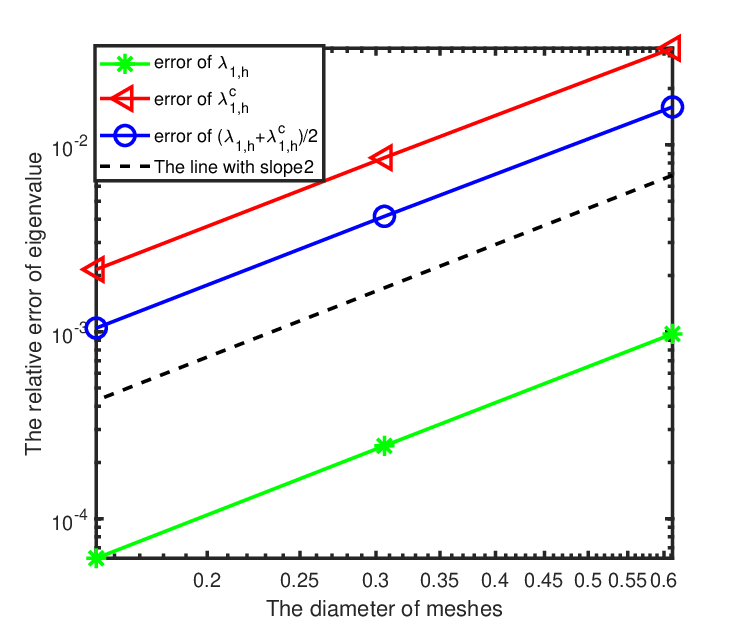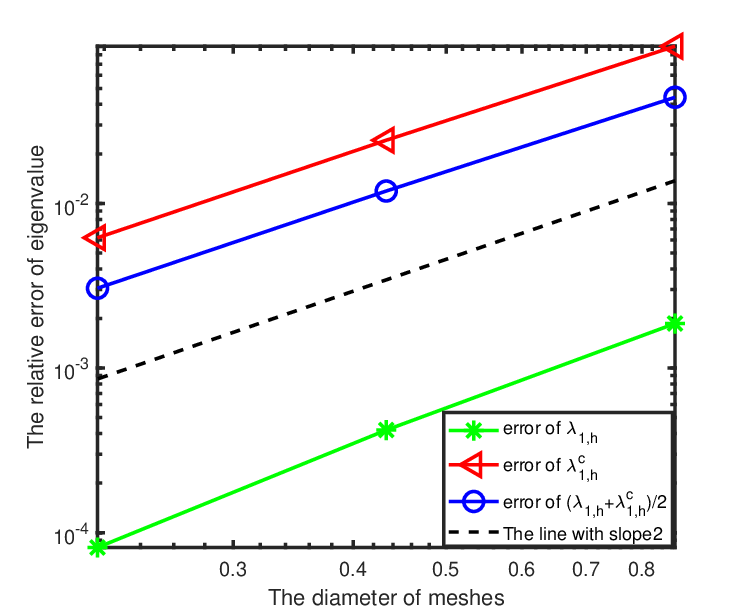We depict the error curves of $\lambda_{1,h}$ , $\lambda^{c}_{1,h}$ and $\frac{\lambda_{1,h}+\lambda^{c}_{1,h}}{2}$ in Figures 1 and 2.
From Table 1, on the one hand, we see that $\lambda_{1,h}$ converge to $\lambda_{1}$ from above and the corrected eigenvalue $\lambda^{c}_{1,h}$ converge to $\lambda_{1}$ from below, which indicate that the correction (3.5) provides lower eigenvalue bounds even though eigenfunctions are smooth. This coincides in the result of Theorem 3.1. On the other hand, on each domain, the CPU time to compute $\lambda^{c}_{1,h}$ is almost the same as that of $\lambda_{1,h}$ , which tell us that the correction takes very little time. Furthermore, from Figures 1 and 2 we see that, on each domain, the error curves of $\lambda^{c}_{1,h}$ and $\lambda_{1,h}$ are parallel to the line with slope 2, which indicate $\lambda^{c}_{1,h}$ and $\lambda_{1,h}$ have the same and optimal convergence order $\mathcal{O}(h^{2})$ and coincide in the result of Theorem 3.2.
Although $\lambda^{c}_{1,h}$ are guaranteed to be the lower bounds of $\lambda_{1}$ whether the eigenfunctions are singular or smooth, compared with $\lambda_{1,h}$ , the accuracy of $\lambda^{c}_{1,h}$ is slightly reduced. Thus, in order to make up the loss of accuracy caused by correction, we use the average $\frac{\lambda_{1,h}+\lambda^{c}_{1,h}}{2}$ as a new approximation. From Figures 1 and 2 we know that, compared with $\lambda^{c}_{1,h}$ , $\frac{\lambda_{1,h}+\lambda^{c}_{1,h}}{2}$ have higher accuracy. Especially, for the square and the hexagon, the errors of $\frac{\lambda_{1,h}+\lambda^{c}_{1,h}}{2}$ are less than or equal to that of $\lambda_{1,h}$ .

Table 1. The uncorrected eigenvalues and the corrected eigenvalues on

\Omega\subset\mathbb{R}^{2}

domain	S		L		H
$h$	$\lambda_{1,h}$	$\lambda^{c}_{1,h}$	$\lambda_{1,h}$	$\lambda^{c}_{1,h}$	$\lambda_{1,h}$	$\lambda^{c}_{1,h}$
$\frac{h_{0}}{32}$	0.24008533	0.24006902	0.34143156	0.34134357	0.39334226	0.39329159
$\frac{h_{0}}{64}$	0.24008065	0.24007657	0.34141986	0.34139787	0.39332055	0.39330788
$\frac{h_{0}}{128}$	0.24007948	0.24007846	0.34141699	0.34141149	0.39331513	0.39331196
$\frac{h_{0}}{256}$	0.24007918	0.24007893	0.34141628	0.34141490	0.39331377	0.39331298
$\frac{h_{0}}{512}$	0.24007911	0.24007905	0.34141610	0.34141576	0.39331344	0.39331324
$t(s)$	31.10	31.20	22.74	22.81	25.34	25.41
Trend	$\searrow$	$\nearrow$	$\searrow$	$\nearrow$	$\searrow$	$\nearrow$

Refer to caption — Figure 1. *The error curves of the first eigenvalues on the unit square (left) and the L-shaped domain (right)*

4.2. Numerical results on $\Omega\subset\mathbb{R}^{3}$

When $\Omega\subset\mathbb{R}^{3}$ , we compute in the cube $(0,1)^{3}$ and the Fichera corner domain $[-1,1]^{3}\setminus(-1,)]^{3}$ . For convenience, we simplify the domains as C and F, respectively. The quasi-uniform mesh samples of the cube and the Fichera corner domain are depicted in Figure 3. In the two domains, we compute the first three eigenvalues using CR finite element and list the results in Table 2. In the cube, $\lambda_{2}$ and $\lambda_{5}$ are eigenvalues with a multiplicity of 3. Corrected eigenvalues $\lambda^{c}_{1,h}$ are listed in Table 3. The error curves are depicted in Figure 4.
From Table 2, we see that, on each domain, $\lambda_{1,h}$ converge to $\lambda_{1}$ from above. From Figure 4, we know that the eigenfunctions corresponding to $\lambda_{1}$ are smooth. This shows that the CR finite element eigenvalue approximations are not necessarily lower bounds in the case of smooth eigenfunctions. From Table 3, we see that, corrected eigenvalues $\lambda^{c}_{1,h}$ converge to $\lambda_{1}$ , which indicate that the correction (3.5) provides lower bounds for eigenvalues even though the eigenfunctions are smooth. From Figure 4, we see that the error curves of $\lambda^{c}_{1,h}$ and $\lambda_{1,h}$ are parallel to the line with slope 2, which indicate $\lambda^{c}_{1,h}$ and $\lambda_{1,h}$ have the same and optimal convergence order $\mathcal{O}(h^{2})$ . The numerical results on three dimensional domains coincide in the result of Theorem 3.1 and Theorem 3.2.

Table 2. The CR finite element eigenvalues approximations on

\Omega\subset\mathbb{R}^{3}

domain	C			F
$h$	$\lambda_{1,h}$	$\lambda_{2,h}$	$\lambda_{5,h}$	$h$	$\lambda_{1,h}$	$\lambda_{2,h}$	$\lambda_{3,h}$
0.6124	0.1623444	1.11356	1.56489	0.8660	0.268747	0.54947	0.72763
0.3062	0.1622261	1.14537	1.65619	0.4330	0.268359	0.56641	0.73377
0.1531	0.1621963	1.15272	1.68222	0.2165	0.268268	0.57235	0.73615
0.0765	0.1621888	1.15448	1.68924	0.1083	0.268247	0.57441	0.73687
Trend	$\searrow$	$\nearrow$	$\nearrow$	–	$\searrow$	$\nearrow$	$\nearrow$

Table 3. The uncorrected eigenvalues and the corrected eigenvalues on

\Omega\subset\mathbb{R}^{3}

domain	C		F
$h$	$\lambda_{1,h}$	$\lambda^{c}_{1,h}$	h	$\lambda_{1,h}$	$\lambda^{c}_{1,h}$
0.6124	0.162344	0.156854	0.8660	0.268747	0.244062
0.3062	0.162226	0.160802	0.4330	0.268359	0.261752
0.1531	0.162196	0.161837	0.2165	0.268268	0.266587
0.0765	0.162189	0.162099	0.1083	0.268247	0.267824
$t(s)$	150.07	150.23	–	223.12	223.26
Trend	$\searrow$	$\nearrow$	–	$\searrow$	$\nearrow$

References

[1] A.E. Alonso, A.D. Russo: Spectral approximation of variationally-posed eigenvalue problems by nonconforming methods, J. Comput. Appl. Math. 223 (2009), 177-197.
[2] M.G. Armentano, R.G. Duran: Asymptotic lower bounds for eigenvalues by nonconforming finite element methods, Electron. Trans. Numer. Anal. 17 (2004), 93-101.
[3] I. Babuska, J.E. Osborn: Eigenvalue Problems. in: Ciarlet, P.G., Lions, J.L. (eds.) Finite Element Methods (Part 1), Handbook of Numerical Analysis, Elsevier Science Publishers, North-Holand 2 (1991), 640-787.
[4] D.Boffi: Finite element approximation of eigenvalue problems, Acta. Numer. 19(2010), 1-120.
[5] S.C. Brenner, L.R. Scott: The Mathematical Theory of Finite Element Methods, 2nd ed. Springer-Verlag, New york, 2002.
[6] C. Carstensen, J. Gedicke, D. Rim: Explicit error estimates for courant, Crouzeix-Raviart and Raviart-Thomas finite element methods, J. Comput. Math. 30 (2012), 337-353.
[7] C. Carstensen, J. Gedicke: Guaranteed lower bounds for eigenvalues, Math. Comput. 83 (2014), 2605-2629.
[8] C.Carstensen, D. Gallistl: Guaranteed lower eigenvalue bounds for the biharmonic equation. Numer. Math. 126 (2014), 33-51.
[9] I. Chavel, E. Feldman: An optimal Poincaré inequality for convex domains of non-negative curvature, Archive for Rational Mechanics and Analysis 65 (1977), 263-273.
[10] L. Chen: iFEM: an innovative finite element methods package in MATLAB, Technical Report, University of California at Irvine (2009).
[11] M. Crouzeix, P.A. Raviart: Conforming and nonconforming finite element methods for solving the stationary stokes equations. RAIRO Anal. Numer. 7(1973), 33-75.
[12] E.M. Garau, P. Morin: Convergence and quasi-optimality of adaptive FEM for Steklov eigenvalue problems, IMA J. Numer. Anal. 1 (2011), 914-946.
[13] J. Hu, Y. Huang: Lower bounds for eigenvalues of the Stokes operator, Adv. Appl. Math. Mech. 5 (2013), 1-18.
[14] J. Hu, Y. Huang, Q. Lin: Lower bounds for eigenvalues of elliptic operators: by nonconforming finite element methods, J. Sci. Comput. 61 (2014), 196-221.
[15] J. Hu, Y. Huang, R. Ma: Guaranteed lower bounds for eigenvalues of elliptic operators, J. Sci. Comput. 67 (2016), 1181-1197.
[16] Q. Li, Q. Lin, H. Xie: Nonconforming finite element approximations of the Steklov eigenvalue problem and its lower bound approximations, Appl. Math. 58 (2013), 129-151.
[17] Y. Li: Lower approximation of eigenvalue by the nonconforming finite element method, J. Math. Numer. Sin. 30 (2008), 195-200.
[18] Q. Li, X. Liu: Explicit finite element error estimates for nonhomogeneous neumann problems, Appl. Math. 63 (2018), 367-379.
[19] Q. Lin, H.T. Huang, Z.C. Li: New expansions of numerical eigenvalues for $-\triangle u=\lambda pu$ by nonconforming element, Math. Comput. 77 (2008), 2061-2084.
[20] Q. Lin, H. Xie, F. Luo, Y. Li, Y. Yang: Stokes eigenvalue approximations from Below with nonconforming mixed finite element methods, Math. Pract. Theory(in Chinese) 40 (2010), 157-168.
[21] Q. Lin, H. Xie: Recent result on lower bounds of eigenvalue problems by nonconforming finte element methods, Inverse Probl. Imag. 7 (2013), 795-811.
[22] X. Liu: A framework of verified eigenvalue bounds for self-adjoint differential operators, Appl. Math. Comput. 267 (2015), 341-355.
[23] F.S. Luo, Q. Lin, H. Xie: Computing the lower and upper bounds of Laplace eigenvalue problem: by combining conforming and nonconforming finite elementmethods. Sci. ChinaMath. 55 (2012), 1069-1082.
[24] J.T. Oden, J.N. Reddy: An introduction to the mathematical theory of finite elements. Courier Dover Publications, New York (2012).
[25] A.D. Russo, A.E. Alonso: A posteriori error estimates for nonconforming approximations of Steklov eigenvalue problems. Comput. Math. Appl. 62(2011), 4100-4117.
[26] G. Savaré: Regularity results for elliptic equations in Lipschitz domains, J. Funct. Anal. 152 (1998), 176-201.
[27] I. Šebestová, T. Vejchodský: Two-Sided bounds for eigenvalues of differential operators with applications to Friedrichs, Poincaré, Trace, and similar constants, J. Funct. Anal. 152 (1998), 176-201.
[28] M. Xie, H. Xie, X. Liu: Explicit lower bounds for Stokes eigenvalue problems by using nonconforming finite elements, JPN J. Ind. Appl. Math. 35 (2018), 1-20.
[29] Y. Yang, Q. Lin, H. Bi, Q. Li: Lower eigenvalues approximation by Morley elements, Adv. Comput. Math. 36 (2012), 443-450.
[30] Y. Yang, Q. Li, S. Li: Nonconforming finite element approximations of the Steklov eigenvalue problem, Appl. Numer. Math. 59 (2009), 2388-2401.
[31] Y. Yang, Z. Zhang, F. Lin: Eigenvalue approximation from below using non-conforming finite elements, Sci. China. Math. 53 (2010), 137-150.
[32] Y. Yang, J. Han, H. Bi, Y. Yu: The lower/upper bound property of the nonoconforming Crouzeix-Raviart element eigenvalues on adaptive meshes, J. Sci. Comput. 62 (2015), 284-299.
[33] Y. Yang, Y. Zhang, H. Bi: Non-conforming Crouzeix-Raviar element approximation for Stekloff eigenvalues in inverse scattering. arXiv:1808.01609 [math.NA] (2018).
[34] C. You, H. Xie, X. Liu: Guaranteed eigenvalue bounds for the Steklov eigenvalue problem, arXiv:1808.08148v1 [math.NA] (2018).
[35] Z. Zhang, Y. Yang, Z. Chen: Eigenvalue approximation from below by Wilsons elements, Chin. J. Numer. Math. Appl. 29 (2007), 81-84.

Authors’ addresses:
Yu Zhang, School of Mathematical Sciences, Guizhou Normal University, Guiyang 550001, China;
School of Mathematics $\&$ Statistics, Guizhou University of Finance and Economics, Guiyang 550001, China. e-mail: zhang_hello_hi@126.com.
Hai Bi, School of Mathematical Sciences, Guizhou Normal University, Guiyang 550001, China. e-mail: bihaimath@gznu.edu.cn.
Yidu Yang (corresponding author), School of Mathematical Sciences, Guizhou Normal University, Guiyang 550001, China. e-mail: ydyang@gznu.edu.cn.