Single-Frequency Imaging and Material Characterization using Reconfigurable Reflectarrays

To get the simulated target profile, all surfaces of the feeding horn apertures, patches on the reflectarrays, and target are discretized into triangular facets. According to the exact free-space near-field equation described in [51], the incident electric field ${\bf{E}}_{\mathrm{inc}}\left({\bf{r}}\right)$ and magnetic field ${\bf{H}}_{\mathrm{inc}}\left({\bf{r}}\right)$ at an observation point ${\bf{r}}$ can be computed using the electric ${{\bf{J}}}\left({\bf{r^{\prime}}}\right)$ and magnetic ${{\bf{M}}}\left({\bf{r^{\prime}}}\right)$ current sources, namely,

where $A_{1}=\frac{{j}{\eta_{0}}}{{4\pi{k_{0}}}}$; $A_{2}=\frac{{j}}{{4\pi{k_{0}}{\eta_{0}^{2}}}}$; $B_{1}=B_{2}=\frac{1}{{4{\pi}}}$; ${G_{1}}=\frac{{-1-j{k_{0}}R+{{\left({{k_{0}}R}\right)}^{2}}}}{{{R^{3}}}}$; ${G_{2}}=\frac{{3+j3{k_{0}}R-{{\left({{k_{0}}R}\right)}^{2}}}}{{{R^{5}}}}$; ${G_{3}}=\frac{{1+j{k_{0}}R}}{{{R^{3}}}}$; ${\bf{R}}={\bf{r}}-{\bf{r^{\prime}}}$, $R=\left|{\bf{R}}\right|$; $k_{0}$ and $\eta_{0}$ are the wave number and impedance in free-space, respectively; ${\bf{r}}$ is the observation point; ${\bf{r^{\prime}}}$ is the source point; and $S$ is surface of the feeding antenna aperture.

With the incident fields ${\bf{E_{\mathrm{inc}}}}$ and ${\bf{H_{\mathrm{inc}}}}$, the induced electric ${\bf{J}}$ and magnetic ${\bf{M}}$ currents on any interface can be calculated using the modified equivalent current approximation (MECA) equations [52, 53], which represents a generalization of the PO for both conducting and non-conducting dielectric surfaces:

where the incident electric field is decomposed into its transverse electric (TE) and transverse magnetic (TM) modes, and analyzed individually; $S_{B}$ is the interface between the two media; ${\eta_{1}}$ is the wave impendence of the outwards medium; ${{{{\bf{\hat{n}}}}_{0}}}$ is the outward unit vector perpendicular to the interface; ${\theta_{\mathrm{inc}}}$ is the incident angle; $E_{\mathrm{inc}}^{\mathrm{TE}\mathrm{/}\mathrm{TM}}$ and ${{{\bf{\hat{e}}}}_{\mathrm{TE}/\mathrm{TM}}}$ are the incident field magnitude and the corresponding unit vector of the TE/TM mode, respectively; and $R_{\mathrm{TE}\mathrm{/}\mathrm{TM}}$ is the reflection coefficient of the TE/TM mode on the interface, which is defined as

where ${\varepsilon_{1}}$ and ${\varepsilon_{2}}$ are the complex permittivity of the outwards and inner medium, respectively, and ${\mu_{1}}$ and ${\mu_{2}}$ are the corresponding permeabilities assumed to be equal. Note that on the surface of the PEC, magnetic current ${{\bf{M}}}=0$ due to the fact that $R_{\mathrm{TE}}=R_{\mathrm{TM}}=-1$. Therefore, the magnetic currents on the feeding antenna apertures, the patch elements on the reflectarrays, and the human body are neglected.

As shown in Fig. 2, assuming the total number of the patches on each reflectarray is $M$ and the electric current distribution of $p$-th feeding antenna is ${{\bf{J}}_{p}^{\mathrm{inc}}}$ $(p\in\{1,2,\dots,P\})$, the incident electric ${{\bf{E}}_{m,p}^{\mathrm{patch}}}$ and magnetic ${{\bf{H}}_{m,p}^{\mathrm{patch}}}$ fields on the $m$-th patch $(m\in\{1,2,\dots,M\})$ can be obtained using Eq. (1). The corresponding induced electric current ${{\bf{J}}_{m,p}^{\mathrm{patch}}}$ can be calculated based on Eq. (2).

The reflectarrays are confocally set to focus the incident wave front to a desired point by using the binary phase approximation, namely, introducing a phase compensation $\Delta\psi_{n,m,p}$ to each patch element,

where ${\rm{mod}}(\cdot)$ is the modulus operator, and $L_{n,m,p}=\left({\left|{{\bf{r}}_{p}^{{\rm{feed}}}-{{\bf{r}}_{m,p}^{{\rm{patch}}}}}\right|+\left|{{{\bf{r}}_{m,p}^{{\rm{patch}}}}-{\bf{r}}_{n}^{{\rm{focus}}}}\right|}\right)$. ${\bf{r}}_{p}^{{\rm{feed}}}$, ${\bf{r}}_{m,p}^{{\rm{patch}}}$, and ${\bf{r}}_{n}^{{\rm{focus}}}$ are the positions of the $p$-th feeding antenna, the $m$-th patch of the $p$-th reflectarray, and the $n$-th focusing point, respectively. Therefore, the electric current is modified as ${{\bf{J}}_{m,p}^{\mathrm{patch}}}{e^{j\Delta\psi_{n,m,p}}}$. Using Eq. (1) again, we can calculate the incident electric ${{\bf{E}}_{m,n,p}^{\mathrm{target}}}$ and magnetic ${{\bf{H}}_{m,n,p}^{\mathrm{target}}}$ fields on the target surface. Thus, the total incident electric ${{\bf{E}}_{n,p}^{\mathrm{target}}}$ and magnetic ${{\bf{H}}_{n,p}^{\mathrm{target}}}$ fields for the $p$-th feeding antenna and the $n$-th focusing point are

According to Eq. (2), the corresponding induced electric ${{\bf{J}}_{n,p}^{\mathrm{target}}}$ and magnetic ${{\bf{M}}_{n,p}^{\mathrm{target}}}$ currents can be written as

where ${{\bf{J}}_{n,p}^{\mathrm{\mathrm{obj}}}}$ and ${{\bf{M}}_{n,p}^{\mathrm{\mathrm{obj}}}}$ are the electric and magnetic currents, respectively, on the surface of the dielectric object. Similarly, ${{\bf{J}}_{n,p}^{\mathrm{body}}}$ and ${{\bf{M}}_{n,p}^{\mathrm{body}}}$ are the currents on the surface of the human body. Noticing that ${{\bf{M}}_{n,p}^{\mathrm{body}}}=0$ for the human body (approximated to be PEC), one can calculate ${{\bf{J}}_{n,p}^{\mathrm{body}}}$ using $1^{\mathrm{st}}$-order PO method. While ${{\bf{J}}^{\mathrm{\mathrm{}}}}$/${{\bf{M}}_{n,p}^{\mathrm{\mathrm{obj}}}}$ must be calculated considering multiple reflections within the dielectric object using a $K^{\mathrm{th}}$-order PO method based on Eq. (1) and Eq. (2). The process can be described as

where ${\bf{J}}^{\mathrm{}}$/${\bf{M}}_{n,p,0}^{\mathrm{obj}}$ is denoted as the electric or magnetic currents induced by the initial reflection on the air-object interface $S_{\mathrm{obj}}$; ${\bf{E}}^{\mathrm{}}$/${\bf{H}}_{n,p,k}^{\mathrm{bot}}$ and ${\bf{J}}^{\mathrm{}}$/${\bf{M}}_{n,p,k}^{\mathrm{bot}}$ are the incident fields and the induced currents, respectively, on the object-body interface $S_{\mathrm{bot}}$ after $k$ $(k\in\{1,2,\dots,K-1\})$ reflections within the dielectric object; Similarly, ${\bf{E}}^{\mathrm{}}$/${\bf{H}}_{n,p,k}^{\mathrm{obj}}$ and ${\bf{J}}^{\mathrm{}}$/${\bf{M}}_{n,p,k}^{\mathrm{obj}}$ correspond to the incident fields and the induced currents, respectively, on $S_{\mathrm{obj}}$. Consequently, the total electric ${\bf{J}}_{n,p}^{\mathrm{obj}}$ and magnetic ${\bf{M}}_{n,p}^{\mathrm{obj}}$ currents on $S_{\mathrm{obj}}$ are computed by

As all the reflectarrays are confocally arranged, all the receiving antennas are able to receive the scattered signal. Define ${\bf{E}}_{n,p}^{\mathrm{rec}}$ as the total received electric field from the $p$-th receiving antenna with all $P$ feeding antennas active and the beam focused at the $n$-th point. Although, ${\bf{E}}_{n,p}^{\mathrm{rec}}$ can be calculated via an inverse computational procedure using the PO method from the target to the receiving horns based on Eq. (1) and Eq. (2), in order to improve the computational efficiency, the general reciprocity theorem for multiple-in-multiple-out (MIMO) systems is used as follows:

where $E_{n,p}^{{\rm{rec}}}$ is the amplitude of the received field $\mathbf{E}_{n,p}^{{\rm{rec}}}$, considered to be uniform on the receiving apertures; ${{\bf{J}}_{n}^{\mathrm{target}}}=\sum\limits_{p=1}^{P}{{\bf{J}}_{n,p}^{\mathrm{target}}}$ and ${{\bf{M}}_{n}^{\mathrm{target}}}=\sum\limits_{p=1}^{P}{{\bf{M}}_{n,p}^{\mathrm{target}}}$ are the total induced electric and magnetic currents on the target surface, respectively; and ${\bf{\hat{e}}}_{n,p}^{{\rm{rec}}}$ represents the uniform complex polarization vector of $\mathbf{E}_{n,p}^{{\rm{rec}}}$.

Finally, the target profile can be reconstructed by adding the received electric field $E_{n,p}^{{\rm{rec}}}$ from all $P$ receivers,

and determining the location of the maximum total received field along the $z$-axis, namely,

where $\left({x_{n},y_{n},z_{n}}\right)$ is the location of the $n$-th focusing point.

To ensure real-time prediction and classification of potential threat objects in the reflectarray screening system, it is desired to develop a fully analytical forward model for characterizing the complex relative permittivity of the object under detection[54, 55]. To achieve this, a ray tracing based GO method is proposed to predict the received electric fields $\tilde{E}_{n}^{{\rm{rec}}}$[56]. By sweeping the relative permittivity $\varepsilon_{r}=\varepsilon_{r}^{\prime}-j\varepsilon_{r}^{\prime\prime}$ and the object thickness $T$, $\tilde{E}_{n}^{{\rm{rec}}}(\varepsilon_{r}^{\prime},\varepsilon_{r}^{\prime\prime},T)$ are calculated and compared to the measured $E_{n}^{{\rm{rec}}}$ (or simulated with the full-wave method of multilevel fast multipole algorithm, MLFMA) to find the best matched magnitude and phase responses. Consequently, the corresponding estimated object thickness $\tilde{T}$ and relative permittivity $\tilde{\varepsilon}_{r}=\tilde{\varepsilon}_{r}^{\prime}-j\tilde{\varepsilon}_{r}^{\prime\prime}$ are obtained.

Figure 3 shows the proposed forward model for a multi-reflectarray-based system. For a general analysis, the $p$-th feeding antenna at ${\bf{r}}_{p}^{{\rm{feed}}}$ is assumed to be active, and only the ray that originates from ${\bf{r}}_{p}^{{\rm{feed}}}$ and terminates at the $p^{\prime}$-th feeding antenna in the receiving mode at ${\bf{r}}_{p^{\prime}}^{{\rm{feed}}}$ is considered. Letting the ray at ${\bf{r}}_{p}^{{\rm{feed}}}$ has an amplitude unity of $E_{0}$, the complex incident amplitude $\tilde{E}_{m,p}^{{\rm{patch}}}$ on the $m$-th patch of the $p$-th reflectarray can be computed by considering both magnitude loss and phase delay,

where ${\bf{r}}_{m,p}^{{\rm{patch}}}$ is the position of the $m$-th patch of the $p$-th reflectarray.

Reflected from the $p$-th reflectarray, which is assumed to focus the CW wave at the $n$-th focusing point ${\bf{r}}_{n}^{{\rm{focus}}}$, the ray will reach the air-object interface $S_{\mathrm{obj}}$ at the point ${\bf{r}}_{{\rm{obj}}}$ using ray tracing,

where ${z_{\mathrm{bg}}}$ is the range of the object-body interface $S_{\mathrm{bot}}$; $T$ is the thickness of the dielectric object; and ${{\theta_{n,m}^{{\rm{inc}}}}}$ is the incident angle. Thus, the ray amplitude at ${\bf{r}}_{{\rm{obj}}}$ can be expressed as

where $\Delta\psi_{n,m,p}$ is the binary phase shift added on the $m$-th patch element of the $p$-th reflectarray when focusing at ${\bf{r}}_{n}^{{\rm{focus}}}$, which is defined in Eq. (III-A).

Scattered by both the dielectric and body surfaces, considering multiple reflections within the dielectric object, the backwards ray will illuminate upon the $m^{\prime}$-th patch of the $p^{\prime}$-th reflectarray at ${{\bf{r}}_{m^{\prime},p^{\prime}}^{{\rm{patch}}}}$. Note that the subindexes $m^{\prime}$ and $p^{\prime}$ of ${{\bf{r}}_{m^{\prime},p^{\prime}}^{{\rm{patch}}}}$ can be determined using ray tracing again, which are only dependent on ${{\bf{r}}_{m,p}^{{\rm{patch}}}}$ and ${{\bf{r}}_{\mathrm{obj}}}$. Thus, the ray at ${{\bf{r}}_{m^{\prime},p^{\prime}}^{{\rm{patch}}}}$ will have an amplitude of $\tilde{E}_{n,m,p}^{{\rm{patch}}}$,

where $\Gamma\left({{\theta_{n,m}^{{\rm{inc}}}}}\right)$ is the total reflection coefficient at the air-object interface $S_{\mathrm{obj}}$.

To characterize the total reflection coefficient $\Gamma\left({{\theta_{n,m}^{{\rm{inc}}}}}\right)$, the transmission line model is introduced in Fig. 4. It can be an effective model because (1) the electrically large reflectarray is capable of focusing the incident wave into a tiny spot in the RoI, which is much smaller compared to the object dimensions in the transverse ($x$-$y$) plane so that the edge diffraction effect from the object can be circumvented; and (2) the dielectric object is already in the far-field region of the patch elements in the reflectarrays such that it is suitable to use the plane-wave incidence approximation in the RoI.

Denoting $k_{zi}$, $i\in\{1,2,3\}$, as the wave number in the $z$-direction for the air, dielectric, and body (PEC) layer, respectively, the corresponding characteristic admittance $Y_{i}$ for TE and TM mode can be calculated as follows:

where ${k_{zi}}=\sqrt{k_{0}^{2}{\varepsilon_{ri}}-k_{x}^{2}}$; $k_{0}^{2}={\omega^{2}}\mu{\varepsilon_{0}}$; ${k_{x}}={k_{0}}\sin{{\theta_{m,n}^{{\rm{inc}}}}}$; $\varepsilon_{0}$ and $\mu_{0}$ are the vacuum permittivity and permeability, respectively; and $\varepsilon_{r1}$, $\varepsilon_{r2}$, and $\varepsilon_{r3}$ are the relative permittivities of the air, dielectric object, and PEC, respectively. The input admittance $Y_{\mathrm{in}}$ at the air-dielectric interface can be wrote as

Accordingly, the total reflection coefficient $\Gamma\left({{\theta_{n,m}^{{\rm{inc}}}}}\right)$ is expressed as

With the confocal setup of the reflectarrays, the ray is refocused by the $p^{\prime}$-th reflectarray and directed towards the corresponding $p^{\prime}$-th feeding antenna located at ${{\bf{r}}_{p^{\prime}}^{{\rm{feed}}}}$. The received complex amplitude $\tilde{E}_{n,m,p}^{{\rm{rec}}}$ at ${{\bf{r}}_{p^{\prime}}^{{\rm{feed}}}}$ is

where $\Delta\psi_{n,m^{\prime},p^{\prime}}$ is the binary phase shift added on the $m^{\prime}$-th patch element of the $p^{\prime}$-th reflectarray when refocusing from ${\bf{r}}_{n}^{{\rm{focus}}}$.

Finally, the total received complex amplitude when focusing at ${\bf{r}}_{n}^{{\rm{focus}}}$ can be calculated by a summation:

where $P$ is the total number of FARAs; and $M$ is the total number of patch elements at each reflectarray.

By sweeping $\varepsilon_{r}^{\prime}$ and $\varepsilon_{r}^{\prime\prime}$ of the relative permittivity $\varepsilon_{r}=\varepsilon_{r}^{\prime}-j\varepsilon_{r}^{\prime\prime}$, and the thickness $T$, the GO predicted received amplitude ${{\tilde{E}_{n}^{{\rm{rec}}}}}\left({\varepsilon_{r}^{\prime},\varepsilon_{r}^{\prime\prime},T}\right)$, $n\in[1,N]$, $N$ being the total number of focusing points used in the estimation, are calculated, and compared to the measured ${{E_{n}^{{\rm{rec}}}}}$ to find the best match by means of minimizing the error function $f\left({{\varepsilon_{r}^{\prime}},\varepsilon_{r}^{\prime\prime},T}\right)$, namely

where ${{\tilde{\varepsilon}}_{r}^{\prime}}$, ${{\tilde{\varepsilon}}_{r}^{\prime\prime}}$, and ${\tilde{T}}$ are the estimated object dielectric constant, loss factor, and thickness, respectively; and ${\tilde{E}_{0}^{{\rm{rec}}}}$ and ${E_{0}^{{\rm{rec}}}}$ are the calibration amplitudes to normalize the predicted and measured received fields, respectively, which are independent on the dielectric object under detection, and can be measured by focusing the incident wave at a reference plane, located at a range different from or the same as $z_{\mathrm{bg}}$.

First of all, it is important to examine the focusing quality of the reflectarrays based on the point spread function (PSF)[57]. By setting the focusing point at $[500,920,800]$ mm in free-space, the PSF is calculated. Figure 6(a) and 6(b) show the 3D and 2D radiation patterns, respectively. As anticipated, a sharp focusing spot, namely high imaging resolution, is achieved. The $3$-dB width of the focusing spot is near ${\lambda_{0}}/2$ along the $x-$ and $y-$axis, and ${\lambda_{0}}$ along the $z-$axis.

In order to obtain a high calculation efficiency while retaining an acceptable imaging accuracy, the $3^{\mathrm{rd}}$-order PO is used to calculate the electric and magnetic currents on the dielectric object surface, namely applying Eq. (12) with $K=3$.

First, two pure dielectric (lossless) objects are considered in the simulation. Object$-1$ has a thickness of $T_{1}=20$ mm and relative permittivity of $\varepsilon_{r1}=8.0-j0.0$; while Object$-2$ has a thickness of $T_{2}=40$ mm and relative permittivity of $\varepsilon_{r2}=2.0-j0.0$. These two objects, satisfying ${{T_{1}}\sqrt{{{\varepsilon_{r1}^{\prime}}}}={T_{2}}\sqrt{{{\varepsilon_{r2}^{\prime}}}}}$, are selected to verify that the proposed method is able to solve the phase-shift ambiguity[45] without loss of generality.

In addition, the general reciprocity theorem described in Eq. (15) are applied throughout the simulations to improve the computation efficiency. Its effectiveness is validated in Fig. 7, where the received fields, with and without the reciprocity theorem, are in a good agreement for both Object$-1$ and Object$-2$. Figure 7 also verifies that the radiation pattern of the reflectarray in the near-field is range-dependent so that the magnitude and phase responses of the received fields for the two ambiguous objects are distinguished, which shows the effectiveness to discriminate these two objects using the algorithm derived in Eq. (29).

Figure 8(a) and 8(b) show the PO simulated target profiles for Object$-1$ and Object$-2$, respectively, which give the accurate widths, in the $x$-axis, and heights, in the $y$-axis, for both Object$-1$ and Object$-2$. As it is also seen, for Object$-1$ with an actual thickness of $20$ mm, the imaged profile center and thickness are $[x_{\mathrm{c}1},y_{\mathrm{c}1},z_{\mathrm{c}1}]=[500,920,780]$ mm and $800-780=20$ mm, respectively; however, for Object$-2$ that has an actual thickness of $40$ mm, the imaged profile center and thickness are also $[x_{\mathrm{c}2},y_{\mathrm{c}2},z_{\mathrm{c}2}]=[500,920,780]$ mm and $800-780=20$ mm, respectively. This phenomenon is attributed to the multiple reflections inside the dielectric object so that the focusing position, corresponding to the maximum magnitude of the received field along the $z$-axis, is achieved under the front surface of the dielectric object.

When it occurs to a lossy Object$-3$, assuming it has a thickness of $T_{3}=40$ mm and complex relative permittivity of $\varepsilon_{r3}=4.0-j0.2$, the magnitude of the multiple reflected waves inside the lossy dielectric slab are considerably degenerated due to the large propagation loss, $\epsilon_{r}^{\prime\prime}=0.2$. The imaging processing of Object$-3$ can be similar to that of a metallic object, where the $1^{\mathrm{st}}$-order PO method can be sufficient to obtain a quite accurate target profile, and the maximum received field along $z$-axis can be achieved when the focusing position is near the front surface of the dielectric object. Figure 9 shows the PO simulated profile of Object$-3$, where the imaged profile center and thickness are $[x_{\mathrm{c}3},y_{\mathrm{c}3},z_{\mathrm{c}3}]=[500,920,760]$ mm and $800\;\mathrm{mm}-760\;\mathrm{mm}=40\;\mathrm{mm}$, respectively.

Considering all aforementioned simulation cases, for an object made of unknown material, a further estimation algorithm, in addition to the profile reconstruction, is required to estimate not only the object permittivity but also a more precise object thickness.

Applying the material identification method derived in Section III-B, $\varepsilon_{r}^{\prime}$ and $\varepsilon_{r}^{\prime\prime}$ are swept from $2.0$ to $10.0$, and from $0$ to $0.5$, respectively. This sweep range covers most common threat materials, such as narcotics, explosives, and other types of contrabands [58, 59]. The dielectric slab thickness $T$ is swept from $0$ mm to $60$ mm. By determining the imaged profile center $[x_{\mathrm{c}},y_{\mathrm{c}},z_{\mathrm{c}}]$ for each object, the equally spaced focusing points can be selected along the range ($z$-axis),

where $\Delta z=10$ mm is the range resolution of the RoI, and total $N=3$ focusing points are considered for estimating object thickness $\tilde{T}$ and complex relative permittivity ${{\tilde{\varepsilon}}_{r}}={{\tilde{\varepsilon}}_{r}^{\prime}}-j{\tilde{\varepsilon}}_{r}^{\prime\prime}$. The importance for selecting those focusing points is that they always correspond to higher receiving magnitudes compared to the other focusing points along the $z-$axis; therefore, a higher receiving signal-to-noise ratio (SNR) can be achieved for a better estimation accuracy.

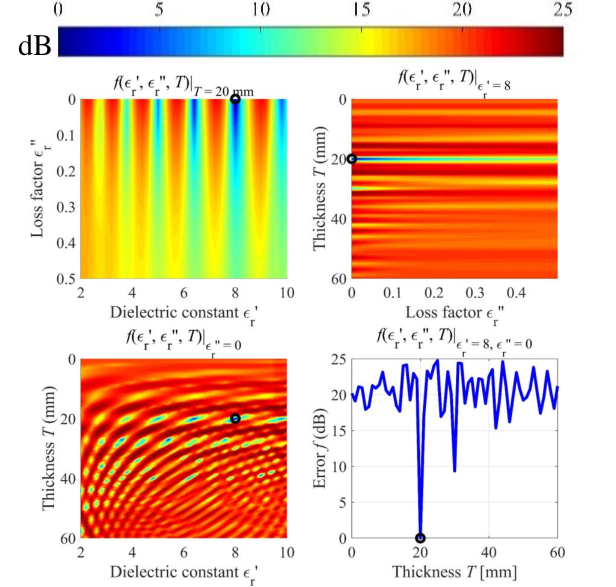
As it is shown in Fig. 10, the best matched magnitude (a) and phase (b) responses, corresponding to the minimum error $\mathrm{min}\left\{f({{\varepsilon_{r}^{\prime}},\varepsilon_{r}^{\prime\prime},T})\right\}$, for Object-$1$ are found at ${{\tilde{\varepsilon}}_{r}^{\prime}}=8.0$, ${\tilde{\varepsilon}}_{r}^{\prime\prime}=0.0$, and $\tilde{T}=20$ mm. These estimated parameters are the same as the actual object thickness and relative permittivity. Note that, although more than three focusing points are presented in this figure for the purpose of verifying the accuracy of the GO predicted field, only the highlighted middle three points are utilized for the estimation. The error distribution $f({{\varepsilon_{r}^{\prime}},\varepsilon_{r}^{\prime\prime},T})$, obtained when sweeping $\varepsilon_{r}^{\prime}$, $\varepsilon_{r}^{\prime\prime}$, and $T$, are shown in Fig. 11, where the achieved minimum error is denoted by a circle.

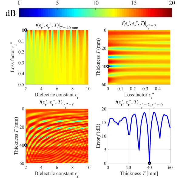
The same estimation process is performed for Object-$2$, and the obtained error distribution is shown in Fig. 12. As it is seen, the minimum error $\mathrm{min}\left\{f({{\varepsilon_{r}^{\prime}},\varepsilon_{r}^{\prime\prime},T})\right\}$ also converges to the actual object parameters $\tilde{\varepsilon}_{r}^{\prime}=2.0$, $\tilde{\varepsilon}_{r}^{\prime\prime}=0.0$, and $\tilde{T}=40$ mm. Therefore, these two ambiguous objects are distinguishable from each other using the proposed estimation method.

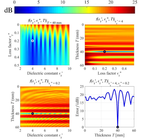
The error distribution $f({{\varepsilon_{r}^{\prime}},\varepsilon_{r}^{\prime\prime},T})$ for the lossy Object-$3$ are shown in Fig. 13, where the minimum error is achieved at $\tilde{\varepsilon}_{r}^{\prime}=4.0$, $\tilde{\varepsilon}_{r}^{\prime\prime}=0.2$, and $\tilde{T}=40$ mm, converging to the actual object parameters again.

Accordingly, aforementioned simulation examples and results verify the proposed imaging scheme that is able to not only image the profiles but also effectively retrieve the complex relative permittivities of the dielectric objects, where a precise object thicknesses can be estimated.

The actual experiment setup to detect a threat object is given in Fig. 14. Denote the dielectric object as Object-$4$. It is a dielectric slab made of polyamide-6, 6 (PA66), which has a relative dielectric constant of $2.8\sim 3.1$ and a low loss tangent of $\tan\sigma<0.01$ at K-band [60]. The size of the dielectric is $200$ mm $\times$ $150$ mm $\times$ $37$ mm. The dielectric slab is attached to the center of a steel plate by a 1.0 mm ($<{\lambda_{0}}/10$) Velcro layer. To predict the received amplitude $\tilde{E}_{n}^{{\rm{rec}}}({{\varepsilon_{r}^{\prime}},\varepsilon_{r}^{\prime\prime},T})$ using GO forward model described in Fig. 3, the Velcro layer is approximated to be an layer of air with the same thickness $1.0$ mm. Therefore, the transmission line model in Fig. 4 for calculating the total reflection coefficient $\Gamma\left({{\theta_{n,m}^{{\rm{inc}}}}}\right)$ is modified, which includes four cascaded layers, namely air-dielectric-air-PEC.

Figure 15 shows the experimentally reconstructed target profile, which has an imaged thickness of $20$ mm that is much smaller than the actual thickness of $37$ mm. The imaged profile center is at $[500,920,780]$ mm. The reason for this is that the strong multiple reflections within the dielectric slab make the focusing position, corresponding to the maximum magnitude of the received field along the $z$-axis, achieved under the front surface of the dielectric object. This explanation is the same as that for the simulation results in Fig. 8(b).

To estimate the complex relative permittivity $\tilde{\varepsilon}_{r}=\tilde{\varepsilon}_{r}^{\prime}-j\tilde{\varepsilon}_{r}^{\prime\prime}$ and a more precise thickness $\tilde{T}$ of the PA66 slab, $\varepsilon_{r}^{\prime}$, $\varepsilon_{r}^{\prime\prime}$, and $T$ are swept to compute the GO predicted received amplitude $\tilde{E}_{n}^{{\rm{rec}}}(\varepsilon_{r}^{\prime},\varepsilon_{r}^{\prime\prime},T)$, which are then compared to the experimental measurements $E_{n}^{{\rm{rec}}}$ to find the best matched magnitude and phase responses using Eq.(29). The measurement is performed $38$ times and 3 focusing points are considered. Figure 16 shows the best matched magnitude (a) and phase (b) responses between the measured electric fields $E_{n}^{\mathrm{rec}}$ and GO predicted $\tilde{E}_{n}^{\mathrm{rec}}({{\tilde{\varepsilon}_{r}^{\prime}},\tilde{\varepsilon}_{r}^{\prime\prime},\tilde{T}})$, corresponding to the minimum error $\mathrm{min}\left\{f({{\varepsilon_{r}^{\prime}},\varepsilon_{r}^{\prime\prime},T})\right\}$. As we can see, the received field magnitude $E_{2}^{{\rm{rec}}}$, corresponding to the focusing point at the range $z=780$ mm, has the maximum magnitude compared to the measured magnitudes of the other focusing points along the $z$-axis. This is accordance with the experimentally reconstructed target profile, shown in Fig. 15, where the imaged object front surface is located at the range $z=780$ mm.

The estimated results on $\tilde{\varepsilon}_{r}^{\prime}$, $\tilde{\varepsilon}_{r}^{\prime\prime}$, and $\tilde{T}$ of the PA66 slab are given in Fig. 17. As shown in Table I, the mean values for $\tilde{\varepsilon}_{r}^{\prime}$, $\tilde{\varepsilon}_{r}^{\prime\prime}$, and $\tilde{T}$ are $3.012$, $0.014$, and $37.6$ mm, respectively; and the standard deviations for $\tilde{\varepsilon}_{r}^{\prime}$, $\tilde{\varepsilon}_{r}^{\prime\prime}$, and $\tilde{T}$ are $0.425$, $0.009$, and $0.593$ mm, respectively. The estimation error can be attributed to the noisy experimental measurement as well as the approximated model of the four-layer transmission line.

References

- [1] D. M. Sheen, D. L. McMakin, and T. E. Hall, “Three-dimensional millimeter-wave imaging for concealed weapon detection,” IEEE Trans. Microw. Theory Tech., vol. 49, no. 9, pp. 1581–1592, Sep 2001.
- [2] S. S. Ahmed, A. Schiessl, and L. P. Schmidt, “A novel fully electronic active real-time imager based on a planar multistatic sparse array,” IEEE Trans. Microw. Theory Tech., vol. 59, no. 12, pp. 3567–3576, Dec 2011.
- [3] S. S. Ahmed, A. Schiessl, F. Gumbmann, M. Tiebout, S. Methfessel, and L. P. Schmidt, “Advanced microwave imaging,” IEEE Microw. Mag., vol. 13, no. 6, pp. 26–43, Sept 2012.
- [4] J. A. Martinez-Lorenzo, F. Quivira, and C. M. Rappaport, “Sar imaging of suicide bombers wearing concealed explosive threats,” Progress in Electromagnetics Research, vol. 125, pp. 255–272, 2012.
- [5] Y. Rodríguez-Vaqueiro, Y. Álvarez López, B. González-Valdes, J. . Martínez, F. Las-Heras, and C. M. Rappaport, “On the use of compressed sensing techniques for improving multistatic millimeter-wave portal-based personnel screening,” IEEE Trans. Antennas Propag., vol. 62, no. 1, pp. 494–499, Jan 2014.
- [6] P. M. Meaney, K. D. Paulsen, A. Hartov, and R. K. Crane, “Microwave imaging for tissue assessment: initial evaluation in multitarget tissue-equivalent phantoms,” IEEE Trans. Biomed. Eng., vol. 43, no. 9, pp. 878–890, Sept. 1996.
- [7] P. M. Meaney, M. W. Fanning, D. Li, S. P. Poplack, and K. D. Paulsen, “A clinical prototype for active microwave imaging of the breast,” IEEE Trans. Microw. Theory Tech., vol. 48, no. 11, pp. 1841–1853, Nov. 2000.
- [8] E. C. Fear, X. Li, S. C. Hagness, and M. A. Stuchly, “Confocal microwave imaging for breast cancer detection: localization of tumors in three dimensions,” IEEE Trans. Biomed. Eng., vol. 49, no. 8, pp. 812–822, Aug 2002.
- [9] L. Yujiri, M. Shoucri, and P. Moffa, “Passive millimeter wave imaging,” IEEE Microw. Mag., vol. 4, no. 3, pp. 39–50, Sept 2003.
- [10] M. Benedetti, M. Donelli, A. Martini, M. Pastorino, A. Rosani, and A. Massa, “An innovative microwave-imaging technique for nondestructive evaluation: Applications to civil structures monitoring and biological bodies inspection,” IEEE Trans. Instrum. Meas., vol. 55, no. 6, pp. 1878–1884, Dec 2006.
- [11] T. Sleasman, M. Boyarsky, M. F. Imani, T. Fromenteze, J. N. Gollub, and D. R. Smith, “Single-frequency microwave imaging with dynamic metasurface apertures,” J. Opt. Soc. Am. B, vol. 34, no. 8, pp. 1713–1726, Aug 2017.
- [12] J. C. Bolomey, “Recent european developments in active microwave imaging for industrial, scientific, and medical applications,” IEEE Trans. Microw. Theory Tech., vol. 37, no. 12, pp. 2109–2117, Dec 1989.
- [13] B. D. Steinberg and H. M. Subbaram, Microwave imaging techniques. John Wiley Sons, 1991.
- [14] S. R. Cloude and E. Pottier, “A review of target decomposition theorems in radar polarimetry,” IEEE Trans. Geosci. Remote Sens., vol. 34, no. 2, pp. 498–518, Mar 1996.
- [15] E. C. Fear, J. Bourqui, C. Curtis, D. Mew, B. Docktor, and C. Romano, “Microwave breast imaging with a monostatic radar-based system: A study of application to patients,” IEEE Trans. Microw. Theory Tech., vol. 61, no. 5, pp. 2119–2128, May 2013.
- [16] I. Walterscheid, J. H. G. Ender, A. R. Brenner, and O. Loffeld, “Bistatic sar processing and experiments,” IEEE Trans. Geosci. Remote Sens., vol. 44, no. 10, pp. 2710–2717, Oct 2006.
- [17] G. Krieger and A. Moreira, “Spaceborne bi- and multistatic sar: potential and challenges,” IEE Proceedings - Radar, Sonar and Navigation, vol. 153, no. 3, pp. 184–198, June 2006.
- [18] J. S. Herd and M. D. Conway, “The evolution to modern phased array architectures,” Proc. IEEE, vol. 104, no. 3, pp. 519–529, Mar. 2016.
- [19] D. L. Donoho, “Compressed sensing,” IEEE Trans. Inf. Theory, vol. 52, no. 4, pp. 1289–1306, Apr. 2006.
- [20] M. T. Alonso, P. Lopez-Dekker, and J. J. Mallorqui, “A novel strategy for radar imaging based on compressive sensing,” IEEE Trans. Geosci. Remote Sens., vol. 48, no. 12, pp. 4285–4295, Dec 2010.
- [21] M. Soumekh, Synthetic Aperture Radar Signal Processing. Wiley, 1999.
- [22] P. Corredoura, Z. Baharav, B. Taber, and G. Lee, “Millimeter-wave imaging system for personnel screening: scanning points a second and using no moving parts,” Proc. SPIE, vol. 6211, pp. 6211 – 6211 – 8, 2006.
- [23] B. N. Lyons, E. Entchev, and M. K. Crowley, “Reflect-array based mm-wave people screening system,” Proc. SPIE, vol. 8900, pp. 8900 – 8900 – 10, 2013.
- [24] H. Gomez-Sousa and J. A. Martinez-Lorenzo, “Modeling and imaging security threats using a single-frequency adaptable reflect-array,” in Proc. 2017 IEEE International Symposium on Technologies for Homeland Security (HST), Apr. 2017, pp. 1–7.
- [25] M. B. Abdillah, B. Lyons, and E. Entchev, “Identification of potential threat materials using active electromagnetic waves,” Mar. 5 2013, uS Patent 8,390,504.
- [26] J. Huang, “Microstrip reflectarray,” in Antennas and Propagation Society Symposium 1991 Digest, June 1991, pp. 612–615 vol.2.
- [27] D. M. Pozar, S. D. Targonski, and H. D. Syrigos, “Design of millimeter wave microstrip reflectarrays,” IEEE Trans. Antennas Propag., vol. 45, no. 2, pp. 287–296, Feb 1997.
- [28] W. Baukus, “X ray imaging for on-the-body contraband detection,” in Proc. 16th Annual Security Technology Symposium & Exhibition, 2000.
- [29] S. Ahmed, F. Gumbmann, A. Schiessl, M. Reiband, S. Methfessel, C. Maire, A. Cenanovic, O. Ostwald, C. Evers, and L. Schmidt, “Qpass quick personnel automatic safe screening for security enhancement of passengers,” in Proc. Future Security Conf., 2011.
- [30] O. Yurduseven, “Indirect microwave holographic imaging of concealed ordnance for airport security imaging systems,” Progress In Electromagnetics Research, vol. 146, pp. 7–13, 2014.
- [31] B. Gonzalez-Valdes, Y. Alvarez-Lopez, J. A. Martinez-Lorenzo, F. L. H. Andres, and C. M. Rappaport, “Sar processing for profile reconstruction and characterization of dielectric objects on the human body surface,” Progress In Electromagnetics Research, vol. 138, pp. 269–282, 2013.
- [32] Y. Alvarez, B. Gonzalez-Valdes, J. A. Martinez-Lorenzo, C. M. Rappaport, and F. Las-Heras, “Sar imaging-based techniques for low permittivity lossless dielectric bodies characterization,” IEEE Antennas Propag. Mag., vol. 57, no. 2, pp. 267–276, Apr. 2015.
- [33] J. C. Weatherall, J. Barber, and B. T. Smith, “Spectral signatures for identifying explosives with wideband millimeter-wave illumination,” IEEE Trans. Microw. Theory Tech., vol. 64, no. 3, pp. 999–1005, Mar. 2016.
- [34] M. E. Baginski, D. L. Faircloth, and M. D. Deshpande, “Comparison of two optimization techniques for the estimation of complex permittivities of multilayered structures using waveguide measurements,” IEEE Trans. Microw. Theory Tech., vol. 53, no. 10, pp. 3251–3259, Oct 2005.
- [35] A. Zamani and A. M. Abbosh, “Estimation of frequency dispersive complex permittivity seen by each antenna for enhanced multistatic radar medical imaging,” IEEE Trans. Antennas Propag., vol. 65, no. 7, pp. 3702–3711, July 2017.
- [36] D. W. Winters, E. J. Bond, B. D. V. Veen, and S. C. Hagness, “Estimation of the frequency-dependent average dielectric properties of breast tissue using a time-domain inverse scattering technique,” IEEE Trans. Antennas Propag., vol. 54, no. 11, pp. 3517–3528, Nov 2006.
- [37] K. K. M. Chan, A. E. C. Tan, L. Li, and K. Rambabu, “Material characterization of arbitrarily shaped dielectrics based on reflected pulse characteristics,” IEEE Trans. Microw. Theory Tech., vol. 63, no. 5, pp. 1700–1709, May 2015.
- [38] J. Bourqui and E. C. Fear, “System for bulk dielectric permittivity estimation of breast tissues at microwave frequencies,” IEEE Trans. Microw. Theory Tech., vol. 64, no. 9, pp. 3001–3009, Sept 2016.
- [39] B. J. Mohammed, K. S. Bialkowski, and A. M. Abbosh, “Radar-based time-domain head imaging using database of effective dielectric constant,” Electron. Lett., vol. 51, no. 20, pp. 1574–1576, 2015.
- [40] S. Salman, D. Psychoudakis, and J. L. Volakis, “Determining the relative permittivity of deep embedded biological tissues,” IEEE Antennas Wireless Propag. Lett., vol. 11, pp. 1694–1697, 2012.
- [41] M. A. Islam, A. Kiourti, and J. L. Volakis, “A novel method of deep tissue biomedical imaging using a wearable sensor,” IEEE Sensors J., vol. 16, no. 1, pp. 265–270, Jan 2016.
- [42] W. B. Weir, “Automatic measurement of complex dielectric constant and permeability at microwave frequencies,” Proc. IEEE, vol. 62, no. 1, pp. 33–36, Jan 1974.
- [43] R. A. Fenner, E. J. Rothwell, and L. L. Frasch, “A comprehensive analysis of free-space and guided-wave techniques for extracting the permeability and permittivity of materials using reflection-only measurements,” Radio Sci., vol. 47, no. 01, pp. 1–13, Feb. 2012.
- [44] P. Nayeri, A. Z. Elsherbeni, and F. Yang, “Radiation analysis approaches for reflectarray antennas [antenna designer’s notebook],” IEEE Antennas Propag. Mag., vol. 55, no. 1, pp. 127–134, Feb. 2013.
- [45] S. Trabelsi, A. W. Kraszewski, and S. O. Nelson, “Phase-shift ambiguity in microwave dielectric properties measurements,” IEEE Trans. Instrum. Meas., vol. 49, no. 1, pp. 56–60, Feb. 2000.
- [46] J. Roelvink and S. Trabelsi, “Measuring the complex permittivity of thin grain samples by the free-space transmission technique,” in 2012 IEEE International Instrumentation and Measurement Technology Conference Proceedings, May 2012, pp. 310–313.
- [47] K. Y. You, M. S. Sim, H. Mutadza, F. Esa, and Y. L. Chan, “Free-space measurement using explicit, reference-plane and thickness-invariant method for permittivity determination of planar materials,” in 2017 Progress in Electromagnetics Research Symposium - Fall (PIERS - FALL), Nov 2017, pp. 222–228.
- [48] S. V. Hum, M. Okoniewski, and R. J. Davies, “Realizing an electronically tunable reflectarray using varactor diode-tuned elements,” IEEE Microw. Wireless Compon. Lett., vol. 15, no. 6, pp. 422–424, June 2005.
- [49] E. Carrasco, M. Barba, and J. A. Encinar, “X-band reflectarray antenna with switching-beam using pin diodes and gathered elements,” IEEE Trans. Antennas Propag., vol. 60, no. 12, pp. 5700–5708, Dec 2012.
- [50] H. Theissen, C. Dahl, I. Rolfes, and T. Musch, “An electronically reconfigurable reflectarray element based on binary phase shifters for k-band applications,” in Proc. 2016 German Microwave Conference (GeMiC), March 2016, pp. 321–324.
- [51] C. A. Balanis, Advanced Engineering Electromagnetics, 2nd ed. Wiley, 2012.
- [52] J. G. Meana, J. . Martinez-Lorenzo, F. Las-Heras, and C. Rappaport, “Wave scattering by dielectric and lossy materials using the modified equivalent current approximation (meca),” IEEE Trans. Antennas Propag., vol. 58, no. 11, pp. 3757–3761, Nov 2010.
- [53] J. Gutiérrez-Meana, J. Á. Martínez-Lorenzo, and F. Las-Heras, “High frequency techniques: The physical optics approximation and the modified equivalent current approximation (meca),” in Electromagnetic waves propagation in complex matter. InTech, 2011.
- [54] R. G. Kouyoumjian and P. H. Pathak, “A uniform geometrical theory of diffraction for an edge in a perfectly conducting surface,” Proc. IEEE, vol. 62, no. 11, pp. 1448–1461, Nov. 1974.
- [55] P. H. Pathak and R. G. Kouyoumjian, “An analysis of the radiation from apertures in curved surfaces by the geometrical theory of diffraction,” Proc. IEEE, vol. 62, no. 11, pp. 1438–1447, Nov 1974.
- [56] W. Zhang and J. A. Martinez-Lorenzo, “Single-frequency material characterization using a microwave adaptive reflect-array,” in 2018 IEEE International Symposium on Antennas and Propagation USNC/URSI National Radio Science Meeting, July 2018, pp. 1063–1064.
- [57] P. J. Shaw and D. J. Rawlins, “The point-spread function of a confocal microscope: its measurement and use in deconvolution of 3-d data,” Journal of Microscopy, vol. 163, no. 2, pp. 151–165, 1991. [Online]. Available: http://dx.doi.org/10.1111/j.1365-2818.1991.tb03168.x
- [58] D. G. Watters, D. G. Falconer, K. J. Harker, R. Ueberschaer, and A. J. Bahr, “Microwave inspection of luggage for contraband materials using imaging and inverse-scattering algorithms,” Research in Nondestructive Evaluation, vol. 7, no. 2, pp. 153–168, Jun 1995.
- [59] E. M. Hussein and E. J. Waller, “Review of one-side approaches to radiographic imaging for detection of explosives and narcotics,” Radiation Measurements, vol. 29, no. 6, pp. 581 – 591, 1998.
- [60] A. R. Von Hippel, Dielectric materials and applications. New York: Wiley, 1954.