Anomalous Kerr effect in SrRuO3 thin films
Abstract
We study the magneto-optical Kerr effect (MOKE) in SrRuO3 thin films, uncovering wide regimes of wavelength, temperature, and magnetic field where the Kerr rotation is not simply proportional to the magnetization but instead displays two-component behavior. One component of the MOKE signal tracks the average magnetization, while the second “anomalous” component bears a resemblance to anomalies in the Hall resistivity which have been previously reported in skyrmion materials. We present a theory showing that the MOKE anomalies arise from the non-monotonic relation between the Kerr angle and the magnetization, when we average over magnetic domains which proliferate near the coercive field. Our results suggest that inhomogeneous domain formation, rather than skyrmions, may provide a common origin for the observed MOKE and Hall resistivity anomalies.
In magnetic solids, the nontrivial momentum space structure of Bloch bands Thouless et al. 1982; Schnyder et al. 2008; Kitaev 2009; Ryu et al. 2010 reveals itself via the intrinsic anomalous Hall effect which arises due to spin-orbit coupling (SOC) and the band Berry curvature Nagaosa et al. 2010. Remarkably, three-dimensional (3D) magnetic solids can host topological monopole-like singularities of the Berry curvature at Weyl nodes in the dispersion Fang et al. 2003; Wan et al. 2011; Yang et al. 2017; Kübler and Felser 2014. These Weyl nodes can contribute significantly to as seen in metallic antiferromagnets like Mn3X (X = Sn, Ge) Yang et al. 2017; Kübler and Felser 2014, and in metallic ferromagnets such as SrRuO3 where exhibits an unusual non-monotonic temperature dependence as the Weyl nodes approach the Fermi energy via tuning magnetization or temperature Fang et al. 2003; Nagaosa et al. 2010; Chen et al. 2013.
Magnetic solids can also harbor real-space topological textures called skyrmions. Skyrmions imprint a real-space Berry curvature on conduction electrons, inducing a so-called “topological Hall effect” (THE) Neubauer et al. 2009; Lee et al. 2009. Skyrmion crystals and THE have been observed in various materials including MnSi Neubauer et al. 2009; Lee et al. 2009, MnGe Kanazawa et al. 2011, Ir/Fe/Co/Pt multilayers Soumyanarayanan et al. 2017; Legrand et al. 2018; Garlow et al. 2019, and Gd2Pd3Si Kurumaji et al. 2019. In recent work, ultrathin epitaxial films of SrRuO3 have been proposed as an oxide-based platform for hosting nanoscale skyrmions, stabilized by a strong chiral interfacial Dzyaloshinskii-Moriya (IDM) exchange Matsuno et al. 2016; Meng et al. 2019.
Experimental support for skyrmions in ultrathin SrRuO3 films comes from the observation of anomalous bump-like features in near the coercive field while traversing a magnetic hysteresis loop Matsuno et al. 2016; Meng et al. 2019; Pang et al. 2017; Ohuchi et al. 2018; Wang et al. 2018; Qin et al. 2019, similar to THE anomalies seen in other skyrmion materials. However, alternative proposals suggest that the Hall anomalies in this ultrathin limit can arise from the complicated temperature dependence of the intrinsic , together with atomic layer inhomogeneities in the ferromagnetic transition temperature or the coercive field Kan et al. 2018; Gerber 2018; Wang et al. 2020; Malsch et al. 2020. These alternative proposals rely on the momentum-space Berry curvature contribution to the intrinsic Hall effect, but the validity of such theories which simply add up the Hall response of two distinct regions remains unclear.
To assess the importance of momentum-space Berry curvature versus the role of skyrmions, and to further test the validity of these proposals, it is important to examine distinct regimes using new experimental probes. In this Letter, we study the magneto-optical Kerr effect (MOKE) in SrRuO3 films. MOKE is a powerful, contactless, and nondestructive technique with high sensitivity and submicrometer spatial resolution. It has been widely used to study electronic and magnetic properties in magnetic materials and devices Qiu and Bader 2000 and more recently in atomically-thin 2D van der Waals magnets Huang et al. 2017; Gong et al. 2017.
In contrast to previous work, our samples ( nm to nm thick) are far from the ultrathin limit, so the IDM interaction, skyrmions, and atomic layer inhomogeneities, are not expected to play an important role. Remarkably, even in this regime, we discover bump-like anomalies in the MOKE signal over wide ranges of temperature, magnetic field, and frequencies, while the magnetization exhibits normal square-like hysteresis loops. Significantly, this observation contradicts the well-established lore that the polar Kerr rotation is proportional to the macroscopic magnetization in ferromagnetic thin films Matsuno et al. 2016; Ohuchi et al. 2018; Qiu and Bader 2000; Argyres 1955. We describe a controlled theory for the high frequency response, showing that the MOKE anomalies can be semi-quantitatively captured by a combination of the non-monotonic magnetization dependence of the Kerr angle and local averaging over magnetic domains. This experimental discovery of a Kerr anomaly, and its theoretical explanation, constitute the key new significant results of our work.
Experimental observations. – SrRuO3 films were grown using pulsed-laser deposition onto both (LaAlO3)0.3(Sr2TaAlO6)0.7 (LSAT) and SrTiO3 (STO) substrates. In contrast to previous studies which explored ultrathin few unit-cell films, our SrRuO3 films range in thickness from to nm, displaying ferromagnetic order below K Li et al. 2020. Here, we focus on the case of an nm thick film grown on LSAT; see Supplemental Material (SM) sup for data on other films. We have measured the Kerr rotation in these films using a wavelength-tunable pulsed laser (repetition rate: 80 MHz) reduced to low-power (<1 mW) and focused weakly onto a 50 m spot on the sample, with the reflected beam modulated by a photo-elastic modulator and passed through a Wollaston prism into a pair of balanced photodiodes, allowing measurement of both the real and imaginary parts of the Kerr angle. Measurements were done in a typical polar Kerr configuration, with the beam reflected at normal incidence and the external field applied in the out-of-plane direction.
Figure 1 shows measurements of the Kerr rotation at normal incidence, Hall resistance , and magnetization , at temperatures from K to K for an 88 nm thick SrRuO3 sample on LSAT. We show and discuss only the real part of the Kerr rotation at 600, 700, and 800 nm; the imaginary part, and additional data at and nm, can be found in the SM sup. While the magnetization (a) has the shape of a typical hysteresis loop, both (b), and the Kerr rotations at nm (c) and nm (d), show a large additional bump-like contribution similar to the topological contribution seen in systems hosting magnetic skyrmions. Such an additional contribution was also observed in previous measurements on few-unit cell ultrathin films, and was attributed to skyrmions Matsuno et al. 2016; Pang et al. 2017; Ohuchi et al. 2018; Qin et al. 2019; Meng et al. 2019; Wang et al. 2018. For longer wavelengths such as nm (e) and nm (see SM), however, this additional contribution is no longer present in our samples, and tracks the magnetization curve.
In addition to these anomalies, the values of and each at large fields, where the magnetization is uniform, change in very different way as the temperature (and therefore the value of this uniform magnetization) is varied. To see this clearly, we show in (f) these values, which we define as and plotted against the corresponding value of the saturation magnetization . (The subscript denotes “uniform” since the high field regime is expected to have a uniform magnetization across the sample.) For the data at nm and nm, the result of this is approximately linear. Because at these wavelengths the hysteresis loops simply track the magnetization (with no anomalies), we conclude that across all temperatures and field values. For the , nm and nm data, however, there is a clearly nonlinear relationship, including a zero crossing at some for each of them.
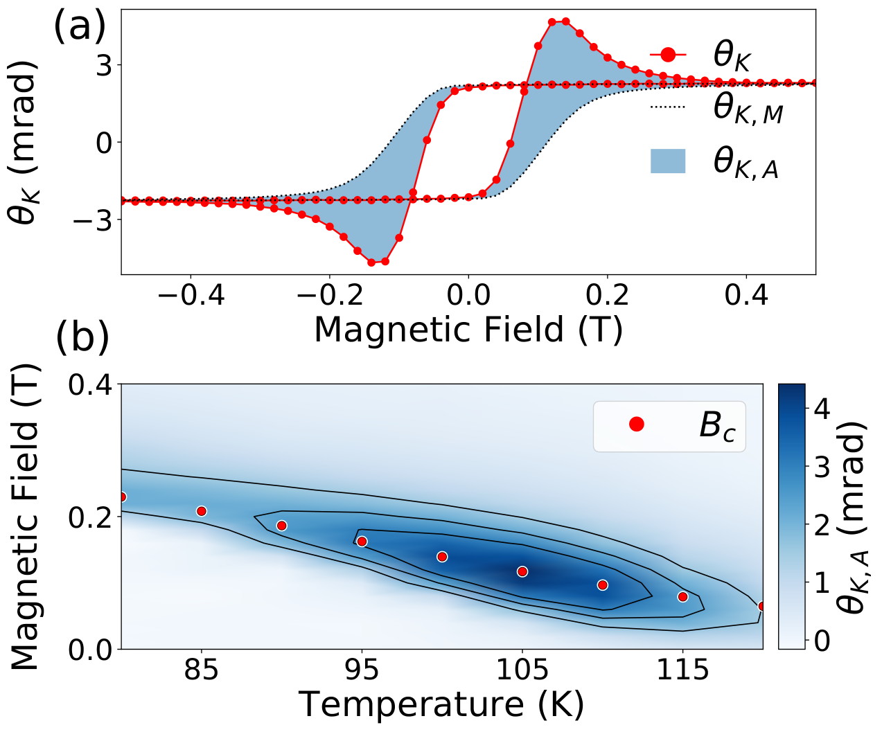
For the MOKE data in which anomalies are present, such as those in Figs. 1(c) and 1(d), the Kerr angle appears to exhibit two components: one component tracks the hysteresis loop (with the proportionality constant potentially changing with temperature, as discussed above), while the second component produces the bump-like anomaly. To see this more clearly, we can separate into a corresponding “normal contribution” , and an additional contribution , which we call the “anomalous Kerr angle”, so that . We illustrate this analysis in Fig. 2 for nm at K, where we obtain by scaling directly measured magnetization data in order to cancel off the Kerr rotation at saturation magnetization [see dashed line in Fig. 2 (a)]. Subtracting this from the nm Kerr signal loop (line with dots) gives a difference signal (blue shaded area) which defines the anomalous Kerr angle . The full field and temperature dependence of quantified in this manner is displayed in Fig. 2(b); the dots indicate the coercive field where the net magnetization vanishes. Here we only show temperatures above 80 K; appears to persist down to very low temperatures but is difficult to clearly extract in this manner, as it becomes relatively small while becomes much larger. We observe that the largest occurs roughly around . It is tempting to assign this feature to skyrmions as they form in the vicinity of magnetization reversals Raju et al. 2019; Meng et al. 2019 in ultrathin films with chiral magnetic interactions. However, SrRuO3 films in our thickness regime possess no known mechanism to stabilize skyrmions, making this an implausible explanation.
We clearly observe the frequency dependence of these anomalies with this analysis. Figure 3 shows both the Kerr rotation at uniform magnetization (as discussed earlier) and the peak value of the anomalous component, , as a function of the photon energy of the laser. Here we also show the imaginary part of the Kerr angle (see SM for more details). We note that the appearance of the anomalies exhibits a resonant behaviour, with a peak at around nm (2 eV) in the real part, and a concomitant zero crossing in the imaginary part consistent with Kramers-Kronig relations.
Similar measurements on films of varying thicknesses yield a nonzero for thicknesses in the range - nm; see SM sup for additional data. In some thinner films ( nm), we observe anomalies in , but not in any of our MOKE measurements. However, in these cases we also do not observe any zero crossings of at non-zero magnetization for the measured , as for the long wavelength data in the nm film. (It is possible that the anomalies may appear at outside the range accessed in our study.) Finally, films grown on LSAT which has greater lattice mismatch (1.4%) with SrRuO3 when compared with the STO substrate (lattice mismatch: 0.45%), exhibit a larger, and broader (in field), . Thus strain has a strong impact on the observed anomalies.
In previous work on anomalies in ultrathin SrRuO3 films, it was suggested that an alternative source (other than skyrmions) for the bumps could be the temperature-dependent sign changes in the bulk anomalous Hall effect combined with inhomogeneities in or the coercive field across the sample Kan et al. 2018. While such inhomogeneities could be important in few unit-cell ultrathin films, where they were proposed to originate from single unit-cell variations in the film thickness, it is less clear that such atomic scale variations can impact the relatively thick films studied in our work. However, a ubiquitous feature common to such magnetic thin films is magnetic domain proliferation near the coercive field Meng et al. 2019; Zahradník et al. 2020. We thus turn to a phenomenological theory of the MOKE in the presence of such domains.
Theory. — As we pass through the coercive field during a magnetization reversal process, minority magnetic domains start to proliferate, and eventually take over the system. During such a process, let be the inhomogeneous local magnetization (perpendicular to the film) at a point in a field . The average magnetization , where denotes the sample volume. Let the Kerr angle in a system with uniform magnetization be given by . We then propose that the measured Kerr angle ; this averaging result in a nontrivial behavior when is a nonlinear function. A heuristic justification for this local magnetization approximation (LMA) for is that the electronic response at high frequency must be local in space. Semiclassically, electrons with Fermi velocity traverse only a distance in a half-period ; using m/s Singh 1996 and eV, yields Å, i.e., on the scale of the lattice spacing. In the SM sup, we compare the LMA with the numerically computed frequency-dependent conductivity tensor from the Kubo formula for a model with spin-orbit coupling using various inhomogeneous magnetization profiles, showing that they quantitatively agree for , where the bandwidth - eV Fang et al. 2003.
We can then compute the Kerr loop in three steps. (i) We simplify the inhomogeneous magnetization profile by two domain types, with magnetizations and perpendicular to the film, and corresponding volume fractions and . Here and . This yields . We fit the magnetization data to extract as a function of . (ii) Next, we assume that the Kerr angle at saturation magnetization is a good proxy for . We thus fit the saturation Kerr angle as a function of saturation magnetization to get . (iii) Finally, using these fitted functions as inputs to the LMA, we obtain the theoretical estimate for the average Kerr angle as .
Figure 4 (a) shows an example of a fit to the magnetization data in an increasing-field sweep (see SM sup for details). We make a simple ansatz for , with , and for large . Thus, which can be read off from the measured , shown as the solid black line in Fig. 4(c). Symmetry dictates , as shown by the solid green line. These two constraints, along with a reasonable ansatz for , allow us to fit , and extract and as shown in Fig. 4(b)-(c). Our results below are robust against variations in the precise shape of .
We next turn to the saturation Kerr angle, , which is measured at a large enough field T to achieve saturation at a given temperature, and then varying the temperature to tune the saturation value of . Figure 4(d) shows a polynomial fit to , which exhibits a non-monotonic behavior similar to the Weyl-node induced non-monotonic Hall resistivity Fang et al. 2003; Nagaosa et al. 2010; Chen et al. 2013.
These key results from the fits in Fig. 4 serve as inputs to the LMA. Figure 5 compares the experimentally measured and the LMA theory results over the hysteresis loop, showing good qualitative agreement in the overall shape and magnitude of the observed bumps. Achieving a better quantitative agreement in terms of the height of the bumps and the precise shapes requires a theory for at each temperature, while we have extracted it using experimental values from different temperature datasets; see SM sup for further discussion of this point.
Such an effective medium approximation fails to explain the anomalies we observe in sup; this discrepancy may be due to the fact that the d.c. conductivity tensor is non-local and expected to be more sensitive to details of the domain size distribution and domain walls. Using a model Hamiltonian, we show in the SM sup that domain walls introduce a correction to which can potentially account for the Hall anomalies.
Conclusion. — We have measured an anomalous contribution to the Kerr signal in thin films of SrRuO3 over wide regimes of magnetic field, temperature, and laser wavelength, which appears to behave similar to anomalies attributed to the THE in skyrmion materials. We have instead shown that these anomalies in the Kerr signal can arise from the non-linear dependence of the Kerr angle on magnetization, together with magnetic domain formation during magnetization reversal. For bulk Hall transport, previous work has shown that the nonmonotonic behavior of the Hall resistivity as a function of magnetization or temperature can arise from Weyl nodes in the band structure Nagaosa et al. 2010; Chen et al. 2013. Weyl nodes, and their interplay with magnetic domain walls, might thus provide a microscopic origin for the non-linear Kerr signal as well as the observed d.c. Hall anomalies. Such an interplay has been recently examined for in the antiferromagnetic Weyl metals Mn3Ge and Mn3Sn Liu and Balents 2017; Li et al. 2019. In light of our results, it would be valuable to also reevaluate the role of magnetic domains versus skyrmions in ultrathin SrRuO3 films.
Acknowledgements.
The optical measurements were performed at Tsinghua University and at the University of Toronto and were supported by the Tsinghua University Startup Fund, the CIFAR Azrieli Global Scholars Programme, NSERC Canada Research Chair, the Canadian Foundation for Innovation, and the Ontario Research Fund. The theoretical studies were performed at the University of Toronto and were funded by NSERC of Canada. This research was enabled in part by support provided by WestGrid (www.westgrid.ca) and Compute Canada Calcul Canada (www.computecanada.ca). Sample growth and characterization were carried out at Tsinghua University and were supported by the Basic Science Center Project of NFSC under grant No. 51788104; the National Basic Research Program of China (grants 2015CB921700 and 2016YFA0301004); and the Beijing Advanced Innovation Center for Future Chip (ICFC).Supplemental Material
TABLE OF CONTENTS
S1. Additional MOKE data for the 88 nm sample at different laser frequencies
S2. MOKE data on different thickness films on STO and LSAT substrates
S3. MOKE measurements at oblique incidence
S4. Alternative model for Hall measurements
S5. Local magnetization approximation (LMA) for optical response
S6. Ansatz for the two-domain model
S7. Impact of modifying the shape of the curves
S8. Impact of domain walls on dc Hall conductivity
I S1. Additional MOKE data for the 88 nm sample at different laser frequencies
For the 88 nm SrRuO3 on LSAT, full datasets of both the real () and imaginary () parts of the Kerr angle as a function of field and temperature were taken at five different wavelengths - 500 nm, 600 nm, 700 nm, 800 nm, and 1500 nm. Here, we show a series of plots analogous to the one shown in Figure 2 of the main text, where an example of raw data at K is shown along with a color plot showing the anomalous part of the signal as a function of both field and temperature, for each of these wavelengths, as well as for the Hall resistivity (Fig. S1).
![[Uncaptioned image]](1908.08974v2/SM_ColourPlots_A.png)

II S2. MOKE data on different thickness films on STO and LSAT substrates
The MOKE signal was strongly affected by the thickness of the samples, as well as the choice of substrate. Figure 7 shows data for a few different samples. Between the two substrates, the STO samples show much smaller and narrower bump features. Between the different thicknesses shown, the difference was mostly in what the temperature range the anomalies occurred, although going to thinner samples (the next being a 51 nm thick sample on LSAT) resulted in these features disappearing entirely. Note that this data set only includes the real part of the Kerr angle, as it was taken on a different setup where only the real part was measured, rather than the full complex Kerr angle as in the other data sets.
III S3. MOKE measurements at oblique incidence
In addition to data taken in the standard polar Kerr configuration, we acquired some data where the laser was reflected from the sample at a large angle of incidence of around 70 degrees while the magnetic field was applied perpendicular to the film as shown schematically in Fig. 8. The s-polarized data (b) is similar to that shown previously, with changing sign just above 95 K. The p-polarized data (a), on the other hand, has which stays fairly constant throughout the temperature range shown. In both cases the additional contribution is clearly visible, as shown in (c) and (d). Despite the dramatic differences in the temperature dependence of , the additional contribution remains similar in sign and magnitude between the different polarizations. Because in our model the anomalies only come from nonlinearity in the versus relationship, this does not necessarily pose a problem. However, we do note that in the usual expressions for a simple out-of-plane magnetization, the p- and s-polarized data would be related by a single overall factor (determined by the angle of incidence and index of refraction), which does not appear to be the case here. This could be due to the presence of in-plane magnetization, as the magnetization axis has been reported to tilt to roughly degrees out of plane Koster et al. 2012.
IV S4. Alternative model for Hall measurements
Recently it was suggested that the Hall effect data on ultrathin SrRuO3 films could be explained by inhomogeneity characterized by a distribution of effective temperatures Kan et al. 2018. Here we discuss why such a “non-intrinsic” explanation of the data in terms of inhomogeneities does not work.
As a simple model, we can write the signal under increasing field as a step function with a temperature dependent saturation value and coercive field strength
| (1) |
We then take the observed signal to be a combination of signals at different temperatures, characterized by a normal distribution with a width
| (2) |
Taking the temperature dependence of and to be approximately linear, and defining parameters and so that and , where is taken to be positive (as is the case physically), gives a solution
| (3) |
where erf and norm are the standard error function and normal distribution respectively. The first term produces a typical magnetization loop, and the second produces features that closely resemble the observed bumps. The constraint of this model, however, that the amplitude and sign of these bump features are set by , as shown in Fig. 9 (a). In our data [Fig. 9 (b)-(e)] the saturation value of the signal decreases with temperature for both and , which means that must be a negative number. While the bumps in the data do indeed also have a negative amplitude, those seen in have a positive amplitude and therefore cannot be explained by the model presented above.
V S5. Local magnetization approximation (LMA) for optical response
The LMA as used in the main text for the measured Kerr angle states that
| (4) |
where is the Kerr angle for a fixed spatially uniform magnetization . This approximation relies on the observation that the conductivity tensor at high frequencies (i.e., optical frequencies) is expected to be spatially local, and may thus be obtained by averaging the local conductivity tensor across the system. In this section, we provide numerical evidence in support of this approximation, by comparing the conductivity tensor for a system with inhomogeneous magnetization calculated (i) using the LMA, i.e., , with (ii) the exact result computed directly using the Kubo formula.
We consider a cubic-lattice electron Hamiltonian, which has been used to study the anomalous Hall effect in metallic ferromagnets Chen et al. 2013, and introduce a spatially varying Weiss field which produces an inhomogeneous exchange splitting and magnetization:
| (5) | |||||
| (6) |
where is the on-site spin-orbit coupling strength, is the angular momentum operator in the basis, and is the spin operator. In , the first term denotes the amplitudes for intra-orbital nearest-neighbor hopping, while refers to next-neighbor inter-orbital hopping amplitudes, and we sum over the orbital index which corresponds respectively to the and orbitals.
The hopping integral is labelled by the bond index , which can take three values corresponding to the unit vectors in the x, y and z-direction, i.e., for . Explicitly, . The inter-orbital hopping occurs on six bonds: , and . The corresponding hopping integrals are given by . In the rest of this section, we discuss the results for the case where the Weiss field is chosen to be uniform in the direction, but has strong inhomogeneity in the -plane. We do this by going to momentum space assuming a super-cell having unit-cell dimension .
The Kubo formula for the conductivity tensor of the inhomogeneous (super-cell) system is given by Mahan 2000; *coleman; *zhang:
| (7) |
where are matrix elements of the velocity operator, and is a Bloch state with an eigenvalue given the super-cell configuration, is the Fermi function and is a small broadening.
We will compare this with the LMA response tensor, which corresponds to a local averaging:
| (8) |
where is the set of easily calculable homogeneous Kubo formula conductivity tensors assuming that the local Weiss field is uniformly applied across the entire system.

Figure 10 presents the comparison between the exact Kubo formula super-cell calculation and the LMA for different inhomogeneous Weiss field configurations. The topmost row shows the unit cells of three super-cell profiles. Dots (blue) and crosses (red) denote the positive and negative z-direction of the Weiss field respectively, while the intensity of the color denotes the magnitude of the Weiss field. Below each configuration, we plot the corresponding conductivity tensor, showing its different components. We observe that LMA results (blue) and the exact results (red) agree well with each other in the large frequency limit, e.g. , for all the tensor components. This corresponds to , where the bandwidth . We have also found good agreement for other sets of model parameters and electronic densities, so the LMA appears to be a robust approximation for the optical conductivity tensor.
Turning to the polar Kerr angle , this is related to the dielectric functions via Argyres 1955
| (9) |
where the dielectric function depends on the conductivity through the following relation . is the background dielectric, and is the vacuum permittivity. For SrRuO3 in the optical frequency regime, the denominator, which involves only the longitudinal component , appears less sensitive to the temperature or the magnetization (e.g., it exhibits no sign changes), and hence less sensitive to the Weiss field. This has been reported in Ref. Kostic et al. 1998 (see also the flat temperature dependence in the optical regime of an empirical expression for in Ref. Dodge et al. 2000). Thus is closely tied to , and we may then directly apply the LMA to the Kerr angle as in Eq. (4). (In our calculations above, we have assumed that the magnetization is linearly proportional to the Weiss field, which we have checked is correct for the regime of interest). The LMA is thus a useful approximation for studying Kerr angle in the optical regime in the presence of magnetic domains as discussed in the main text.
VI S6. Ansatz for the two-domain model and magnetization fits
The two-domain model is a simplified description for the domain evolution during the magnetization reversal near the coercive magnetic field. As described in the main text, the model characterizes a magnetization profile by replacing the positive domains having positive z-component magnetization with an effective value while replacing the negative domains with an effective value . The volume fraction of the positive domain is denoted by , so the negative domain has a volume fraction .
Consider an increasing-field sweep starting from a sufficiently large negative field to a large positive field during which the magnetization begins from a uniform value and eventually reaches a uniform value , passing through a magnetization reversal region where minority magnetic domains grow and proliferate. For our data, we can set Tesla. We can conveniently divide the field range into two regimes: (1) a negatively uniform regime where , and (2) a magnetization-reversal regime where increases towards while drops to zero. In the uniform regime with , the field dependence of is directly given by the experimentally measured magnetization , namely in regime (1). In the rest of this section, we construct ansatz for and in the regime .
The ansatz for in an increasing-field sweep must satisfy two constraints. First, it must obey boundary conditions: and . Second, in the presence of the positive applied field, it should be monotonically increasing with . We assume that follows a modified hyperbolic tangent function (shifted and rescaled), as given below.
| (10) |
The parameters and determine the behaviour of . Physically, is roughly set by the coercive field, while a smaller results in a more rapid change of as we go across . The envelope function with is needed to account for a slow increase of the magnetization near the end of the magnetization-reversal regime approaching .
Turning next to the ansatz for , we will use time-reversal symmetry to set , which is thus fully determined from the experiment. Furthermore, since at this field. The impact of a positive field on is unknown. We assume that the field dependence of has a similar tanh form, decreasing from the experimentally measured to a value smaller in magnitude at , where . This can be achieved by the following function:
| (11) |
where we use the same simple tanh functional form as before, but with different fit parameters and . We determine the ansatz parameters by fitting the average magnetization curve obtained from the model to the experimental curve. The results are then used to compute the Kerr angle: , where is the Kerr angle as a function of the uniform magnetization as defined in the main text. The result of the decreasing field sweep is then taken to be the time-reversal counterpart of that in the increasing-field sweep, namely . Figure 11 illustrates two examples of the fitting, and the ansatz corresponding to the Kerr angle plots at 115K and 120K in the main text.
VII S7. Impact of modifying the shape of the curves
An essential input to our phenomenological theory is the magnetization dependence of the Kerr angle in a uniform magnetization profile, i.e., . In the main text, we extract this from the experiment, by measuring the Kerr angle in a large applied field, while tuning via temperature. This leads to a good qualitative agreement between the theory and the experiment. However, the model in fact requires as input an isothermal curve, which is beyond the scope of our current study. Instead, we show in Fig. 12 how assuming that the isothermal curve deviates slightly from the experimental curve, can lead to a better quantitative agreement with the measured Kerr anomaly. The proposed isothermal curves are indicated by the dashed lines in panel (a), which terminate at the experimental data points at the corresponding temperature (e.g., the proposed K green curve touches the experimental black curve at K).
VIII S8. Impact of domain walls on dc Hall conductivity
In this section, we show from a numerical computation using the Kubo formula that the dc Hall conductivity exhibits a domain wall contribution , which may explain the Hall anomalies observed during magnetization reversal in our experiment.
We first compute the Hall resistivity hysteresis loop using an effective medium approximation (EMA) Stroud 1975, which is a well known approximation for computing dc transport coefficients in an inhomogeneous system. Since dc transport is non-local, the EMA may be viewed as the appropriate dc generalization of the LMA. Its formalism relies on solving Maxwell’s equations with matching boundary conditions between constituents of the inhomogeneous system with well-defined local dc transport coefficients Stroud 1975. For simplicity, we deploy the spherical-inclusion version of EMA Granovsky et al. 1994. Using the fitting functions and from the anomalous Kerr calculation and the curve of versus magnetization from Fig. 1(f) in the main text, we can similarly compute the hysteresis loop for the Hall resistivity. The result is shown in Fig. 13 in comparison with the experimental data at 120 K. There are no obvious bump features in the EMA hysteresis loop. In the increasing-field sweep, a negative correction is needed to account for the anomalies. Below, we show that there can be a domain-wall correction arising from quantum mechanical effects beyond the EMA. We find that the domain wall contribution to the Hall conductivity has a positive sign for positive magnetization, which implies a negative correction to the Hall resistivity in an increasing field sweep. This domain wall contribution, which is expected to become more important near the magnetization reversal, may thus account for the observed anomalous dip in in the increasing field sweep.
We consider the cubic-lattice Hamiltonian, Eq. (6), placed on a geometry with open boundaries in the x-direction and periodic boundary conditions in the y and z-direction, as illustrated in Fig. 15(b). We choose the hopping parameters such that the Hall conductivity exhibits a nonmonotonic dependence on the Weiss field , as shown in Fig. 14(a), similar to that observed in the experiment (see versus magnetization in Fig. 1 in the main text). We note that the sign of here is identified with that of in the experiment. We identify the Weiss field here with the magnetization, and we have checked numerically that they are indeed proportional to each other in the case with uniform Weiss-field configurations. This simple model is useful since it qualitatively captures the sign of the Hall effect in SrRuO3, and its change with magnetization, although we do not expect it to quantitatively explain the experimental data.
We next introduce a sharp domain wall in the yz-plane, as shown in Fig. 15(a), which divides the system into two equal domains with two Weiss fields: . We consider the regime where , following our fits to the magnetization data in the regime of the increasing field sweep. We then compute using two methods: (1) exact Kubo formula and (2) the effective medium approximation. In the latter, we use the response functions from the uniform calculation done in Fig. 14 as the inputs. We identify the difference between the result from these two calculations as the domain wall contribution to the Hall conductivity: .
Figure 15(b)-(f) shows the Hall conductivity in the regime for various values of . We find that the Kubo formula result lies above the EMA result, and we thus infer a positive the domain-wall correction . This is precisely the correct sign needed to account for the Hall anomalies. In literature, the nonmonotonicity in the Hall effect with varying the uniform magnetization has been shown to arise from topological Weyl points in the band structure Chen et al. 2013, so it is possible that the Hall anomaly may be the result of an interplay between the Weyl points and the magnetic domain walls. Indeed, domain walls have been shown in Refs. Liu and Balents 2017; Li et al. 2019 to enhance the Hall effect for antiferromagnetic Weyl metals Mn3Ge and Mn3Sn. We will discuss this interplay for a model ferromagnetic Weyl metal in a future publication.
References
- Thouless et al. (1982) D. J. Thouless, M. Kohmoto, M. P. Nightingale, and M. den Nijs, Phys. Rev. Lett. 49, 405 (1982).
- Schnyder et al. (2008) A. P. Schnyder, S. Ryu, A. Furusaki, and A. W. W. Ludwig, Phys. Rev. B 78, 195125 (2008).
- Kitaev (2009) A. Kitaev, AIP Conference Proceedings 1134, 22 (2009).
- Ryu et al. (2010) S. Ryu, A. P. Schnyder, A. Furusaki, and A. W. W. Ludwig, New Journal of Physics 12, 065010 (2010).
- Nagaosa et al. (2010) N. Nagaosa, J. Sinova, S. Onoda, A. H. MacDonald, and N. P. Ong, Rev. Mod. Phys. 82, 1539 (2010).
- Fang et al. (2003) Z. Fang, N. Nagaosa, K. S. Takahashi, A. Asamitsu, R. Mathieu, T. Ogasawara, H. Yamada, M. Kawasaki, Y. Tokura, and K. Terakura, Science 302, 92 (2003).
- Wan et al. (2011) X. Wan, A. M. Turner, A. Vishwanath, and S. Y. Savrasov, Phys. Rev. B 83, 205101 (2011).
- Yang et al. (2017) H. Yang, Y. Sun, Y. Zhang, W.-J. Shi, S. S. P. Parkin, and B. Yan, New Journal of Physics 19, 015008 (2017).
- Kübler and Felser (2014) J. Kübler and C. Felser, EPL (Europhysics Letters) 108, 67001 (2014).
- Chen et al. (2013) Y. Chen, D. L. Bergman, and A. A. Burkov, Phys. Rev. B 88, 125110 (2013).
- Neubauer et al. (2009) A. Neubauer, C. Pfleiderer, B. Binz, A. Rosch, R. Ritz, P. G. Niklowitz, and P. Böni, Phys. Rev. Lett. 102, 186602 (2009).
- Lee et al. (2009) M. Lee, W. Kang, Y. Onose, Y. Tokura, and N. P. Ong, Phys. Rev. Lett. 102, 186601 (2009).
- Kanazawa et al. (2011) N. Kanazawa, Y. Onose, T. Arima, D. Okuyama, K. Ohoyama, S. Wakimoto, K. Kakurai, S. Ishiwata, and Y. Tokura, Phys. Rev. Lett. 106, 156603 (2011).
- Soumyanarayanan et al. (2017) A. Soumyanarayanan, M. Raju, A. L. Gonzalez Oyarce, A. K. C. Tan, M.-Y. Im, A. P. Petrović, P. Ho, K. H. Khoo, M. Tran, C. K. Gan, F. Ernult, and C. Panagopoulos, Nat. Mater. 16, 898 (2017).
- Legrand et al. (2018) W. Legrand, J.-Y. Chauleau, D. Maccariello, N. Reyren, S. Collin, K. Bouzehouane, N. Jaouen, V. Cros, and A. Fert, Sci. Adv. 4, eaat0415 (2018).
- Garlow et al. (2019) J. A. Garlow, S. D. Pollard, M. Beleggia, T. Dutta, H. Yang, and Y. Zhu, Phys. Rev. Lett. 122, 237201 (2019).
- Kurumaji et al. (2019) T. Kurumaji, T. Nakajima, M. Hirschberger, A. Kikkawa, Y. Yamasaki, H. Sagayama, H. Nakao, Y. Taguchi, T.-h. Arima, and Y. Tokura, Science 365, 914 (2019).
- Matsuno et al. (2016) J. Matsuno, N. Ogawa, K. Yasuda, F. Kagawa, W. Koshibae, N. Nagaosa, Y. Tokura, and M. Kawasaki, Sci. Adv. 2, e1600304 (2016).
- Meng et al. (2019) K.-Y. Meng, A. S. Ahmed, M. Baćani, A.-O. Mandru, X. Zhao, N. Bagués, B. D. Esser, J. Flores, D. W. McComb, H. J. Hug, and F. Yang, Nano Lett. 19, 3169 (2019).
- Pang et al. (2017) B. Pang, L. Zhang, Y. B. Chen, J. Zhou, S. Yao, S. Zhang, and Y. Chen, ACS Applied Materials & Interfaces 9, 3201 (2017).
- Ohuchi et al. (2018) Y. Ohuchi, J. Matsuno, N. Ogawa, Y. Kozuka, M. Uchida, Y. Tokura, and M. Kawasaki, Nat. Commun. 9, 1 (2018).
- Wang et al. (2018) L. Wang, Q. Feng, Y. Kim, R. Kim, K. H. Lee, S. D. Pollard, Y. J. Shin, H. Zhou, W. Peng, D. Lee, W. Meng, H. Yang, J. H. Han, M. Kim, Q. Lu, and T. W. Noh, Nature Materials 17, 1087 (2018).
- Qin et al. (2019) Q. Qin, L. Liu, W. Lin, X. Shu, Q. Xie, Z. Lim, C. Li, S. He, G. M. Chow, and J. Chen, Advanced Materials 31, 1807008 (2019).
- Kan et al. (2018) D. Kan, T. Moriyama, K. Kobayashi, and Y. Shimakawa, Phys. Rev. B 98, 180408 (2018).
- Gerber (2018) A. Gerber, Phys. Rev. B 98, 214440 (2018).
- Wang et al. (2020) L. Wang, Q. Feng, H. G. Lee, E. K. Ko, Q. Lu, and T. W. Noh, Nano Lett. 20, 2468 (2020).
- Malsch et al. (2020) G. Malsch, D. Ivaneyko, P. Milde, L. Wysocki, L. Yang, P. H. M. van Loosdrecht, I. Lindfors-Vrejoiu, and L. M. Eng, ACS Applied Nano Materials 3, 1182 (2020).
- Qiu and Bader (2000) Z. Q. Qiu and S. D. Bader, Review of Scientific Instruments 71, 1243 (2000).
- Huang et al. (2017) B. Huang, G. Clark, E. Navarro-Moratalla, D. R. Klein, R. Cheng, K. L. Seyler, D. Zhong, E. Schmidgall, M. A. McGuire, D. H. Cobden, W. Yao, D. Xiao, P. Jarillo-Herrero, and X. Xu, Nature 546, 270 (2017).
- Gong et al. (2017) C. Gong, L. Li, Z. Li, H. Ji, A. Stern, Y. Xia, T. Cao, W. Bao, C. Wang, Y. Wang, Z. Q. Qiu, R. J. Cava, S. G. Louie, J. Xia, and X. Zhang, Nature 546, 265 (2017).
- Argyres (1955) P. N. Argyres, Phys. Rev. 97, 334 (1955).
- Li et al. (2020) Z. Li, S. Shen, Z. Tian, K. Hwangbo, M. Wang, Y. Wang, F. M. Bartram, L. He, Y. Lyu, Y. Dong, G. Wan, H. Li, N. Lu, J. Zang, H. Zhou, E. Arenholz, Q. He, L. Yang, W. Luo, and P. Yu, Nat. Commun. 11, 184 (2020).
- (33) See Supplemental Material for details of: (i) additional MOKE data for the 88nm sample at different laser frequencies, (ii) further MOKE data on different thickness films on STO and LSAT substrates, (iii) MOKE measurements at oblique incidence, (iv) discussion of why an alternative “non-intrinsic” explanation of the data in terms of inhomogeneities does not work, (v) numerical check of the validity of LMA at large frequencies, (vi) ansatz for the two-domain model, (vii) discussion on how possible isothermal curve may result in a quantitatively better agreement between the experiment and the theory, and (viii) dc Hall conductivities of a cubic model with magnetic domain walls, showing a domain-wall correction to the Hall conductivity.
- Raju et al. (2019) M. Raju, A. Yagil, A. Soumyanarayanan, A. K. C. Tan, A. Almoalem, F. Ma, O. M. Auslaender, and C. Panagopoulos, Nat. Commun. 10, 696 (2019).
- Zahradník et al. (2020) M. Zahradník, K. Uhlířová, T. Maroutian, G. Kurij, G. Agnus, M. Veis, and P. Lecoeur, Materials and Design 187, 108390 (2020).
- Singh (1996) D. J. Singh, Journal of Applied Physics 79, 4818 (1996).
- Liu and Balents (2017) J. Liu and L. Balents, Phys. Rev. Lett. 119, 087202 (2017).
- Li et al. (2019) X. Li, C. Collignon, L. Xu, H. Zuo, A. Cavanna, U. Gennser, D. Mailly, B. Fauqué, L. Balents, Z. Zhu, and K. Behnia, Nat. Commun. 10, 3021 (2019).
- Koster et al. (2012) G. Koster, L. Klein, W. Siemons, G. Rijnders, J. S. Dodge, C.-B. Eom, D. H. A. Blank, and M. R. Beasley, Rev. Mod. Phys. 84, 253 (2012).
- Mahan (2000) G. Mahan, Many-Particle Physics, Physics of Solids and Liquids (Springer US, 2000).
- Coleman (2015) P. Coleman, Introduction to many-body physics (Cambridge University Press, 2015).
- Scalapino et al. (1993) D. J. Scalapino, S. R. White, and S. Zhang, Phys. Rev. B 47, 7995 (1993).
- Kostic et al. (1998) P. Kostic, Y. Okada, N. C. Collins, Z. Schlesinger, J. W. Reiner, L. Klein, A. Kapitulnik, T. H. Geballe, and M. R. Beasley, Phys. Rev. Lett. 81, 2498 (1998).
- Dodge et al. (2000) J. S. Dodge, C. P. Weber, J. Corson, J. Orenstein, Z. Schlesinger, J. W. Reiner, and M. R. Beasley, Phys. Rev. Lett. 85, 4932 (2000).
- Stroud (1975) D. Stroud, Phys. Rev. B 12, 3368 (1975).
- Granovsky et al. (1994) A. Granovsky, A. Vedyayev, and F. Brouers, Journal of Magnetism and Magnetic Materials 136, 229 (1994).