Exploring anomalous couplings in Higgs boson pair production through shape analysisPreprint: MPP-2019-183
Abstract
We classify shapes of Higgs boson pair invariant mass distributions , calculated at NLO with full top quark mass dependence, and visualise how distinct classes of shapes relate to the underlying coupling parameter space. Our study is based on a five-dimensional parameter space relevant for Higgs boson pair production in a non-linear Effective Field Theory framework. We use two approaches: an analysis based on predefined shape types and a classification into shape clusters based on unsupervised learning. We find that our method based on unsupervised learning is able to capture shape features very well and therefore allows a more detailed study of the impact of anomalous couplings on the shape compared to more conventional approaches to a shape analysis.
Keywords
Higgs phenomenology, Effective Field Theory, machine learning, future colliders1 Introduction
The Higgs sector as we see it today is probably just a glimpse of an underlying more general structure still awaiting to be explored. Manifestations of new physics at higher scales would lead to operators which on one hand introduce new, effective couplings and on the other hand also modify interactions known in the Standard Model (SM). Therefore it is a primary goal for collider physics in the next decades to constrain the couplings, in particular in the Higgs sector, to an unprecedented precision. This is particularly true for the Higgs boson self couplings, in order to find out whether the Higgs potential is indeed of the form assumed by the SM. Deviations from this form could provide strong hints about how to extend the SM.
The trilinear Higgs boson coupling can be constrained by measurements of Higgs boson pair production Aad:2019uzh; Sirunyan:2018two, where the gluon fusion channel yields the largest cross section, and the most stringent 95% CL limits on the total cross section at TeV are currently , constraining trilinear coupling modifications to the range Aad:2019uzh.
The trilinear Higgs couplings can also be constrained in an indirect way, through measurements of processes which are sensitive to these couplings via electroweak corrections McCullough:2013rea; Gorbahn:2016uoy; Degrassi:2016wml; Bizon:2016wgr; Maltoni:2017ims; Kribs:2017znd; Degrassi:2017ucl; Nakamura:2018bli; Kilian:2018bhs; Maltoni:2018ttu; Vryonidou:2018eyv; Gorbahn:2019lwq. Such processes offer important complementary information, however they are susceptible to other BSM couplings entering the loop corrections at the same level, and therefore the limits on extracted this way may be more model dependent than the ones extracted from the direct production of Higgs boson pairs. A corresponding experimental analysis based on single Higgs boson production processes has been performed ATL-PHYS-PUB-2019-009, and recently combined constraints from single and double Higgs boson production became available ATLAS:2019pbo. The idea of indirect constraints through loop corrections also has been employed trying to constrain the quartic Higgs boson self-coupling from (partial) EW corrections to Higgs boson pair production Bizon:2018syu; Borowka:2018pxx.
Theoretical constraints on are rather loose if derived in a largely model independent way. Recent work based on general concepts like vacuum stability and perturbative unitarity suggests that for a new physics scale in the few TeV range Falkowski:2019tft; Chang:2019vez; DiLuzio:2017tfn; DiVita:2017eyz. More specific models can lead to more stringent bounds, see e.g. Refs. Braathen:2019pxr; Basler:2018dac; Babu:2018uik; Adhikary:2017jtu; Lewis:2017dme. Recent phenomenological studies about the precision that could be reached for the trilinear coupling at the (HL-)LHC and future hadron colliders are summarised in Refs. Dawson:2018dcd; Cepeda:2019klc; DiMicco:2019ngk.
Higgs boson pair production in gluon fusion in the SM has been calculated at leading order in Refs. Eboli:1987dy; Glover:1987nx; Plehn:1996wb, and at NLO in the limit, rescaled with the full Born matrix element, in Ref. Dawson:1998py. Ref. Maltoni:2014eza contains the full top quark mass dependence in the real radiation, while the virtual part is calculated in the heavy top limit. The NLO QCD corrections with full top quark mass dependence became available more recently Borowka:2016ehy; Borowka:2016ypz; Baglio:2018lrj; Baglio:2020ini. Implementations of the full NLO QCD corrections in parton shower Monte Carlo programs are also available Heinrich:2017kxx; Jones:2017giv; Heinrich:2019bkc.
NNLO QCD corrections have been computed in the limit in Refs. deFlorian:2013uza; deFlorian:2013jea; Grigo:2014jma; Grigo:2015dia; deFlorian:2016uhr. The calculation of Ref. deFlorian:2016uhr has been combined with results including the top quark mass dependence as far as available in Ref. Grazzini:2018bsd, and the latter has been supplemented by soft gluon resummation in Ref. deFlorian:2018tah. The scale uncertainties at NLO are still at the 10% level, while they are decreased to about 5% when including the NNLO corrections. The uncertainties due to the chosen top mass scheme have been assessed in Ref. Baglio:2018lrj.
Analytic approximations for the top quark mass dependence of the two-loop amplitudes in the NLO calculation have been studied in Refs. Grober:2017uho; Bonciani:2018omm; Xu:2018eos; Davies:2018ood; Davies:2019xzc. Complete analytic results in the high energy limit have been presented in Ref. Davies:2018qvx; the latter have been combined with the full NLO results in the regions where they are more appropriate in Ref. Davies:2019dfy.
The effects of operators within an Effective Field Theory (EFT) description of Higgs boson pair production have been studied at LO QCD in Refs. Contino:2012xk; Goertz:2014qta; Chen:2014xra; Azatov:2015oxa; Dawson:2015oha; Carvalho:2015ttv; Cao:2015oaa; Cao:2016zob; DiVita:2017eyz; deBlas:2018tjm and at NLO in the limit in Refs. Grober:2015cwa; Grober:2016wmf; Maltoni:2016yxb, including also CP-violating operators Grober:2017gut. EFT studies at NNLO in the limit are also available deFlorian:2017qfk. In Ref. Buchalla:2018yce for the first time the full NLO QCD corrections have been combined with an EFT approach to study BSM effects.
It is well known that Higgs boson pair production in gluon fusion is a process where delicate cancellations occur between contributions containing the trilinear Higgs coupling and box-type contributions not containing the trilinear coupling. While the destructive interference between these contributions is usually seen as a curse leading to small cross sections, it can be turned into a virtue when analyzing the shapes of distributions, as for example the di-Higgs invariant mass distribution , because even small anomalous couplings can lead to characteristic shape changes. Therefore it is important to investigate in which way the shapes are influenced by a certain configuration in the coupling parameter space.
The idea of a shape analysis has been pursued already in various ways based on LO studies, see e.g. Refs. Chen:2014xra; Azatov:2015oxa; Dawson:2015oha; Carvalho:2015ttv; Carvalho:2016rys; Carvalho:2017vnu. In Ref. Carvalho:2015ttv, a cluster analysis is proposed to define 12 benchmark points in a 5-dimensional non-linear EFT parameter space which result from clusters of “similar” shapes. The similarity measure in this case is based on a binned likelihood ratio using LO predictions for the observables , and . In Ref. Buchalla:2018yce it was analyzed how the and distributions change when going from LO to NLO for the benchmark points defined in Ref. Carvalho:2015ttv.
As a function of the 5-dimensional coupling parameter space, the distribution can have a few characterising features, such as an enhanced low- region, a double peak, a single peak or an enhanced tail. Some of these features can be attributed rather easily to a certain anomalous coupling, for example, an enhanced low- region is naturally produced by large values of . Other features of the -shape, like a double peak or a SM-like distribution, are harder to attribute to a certain coupling configuration, as there are a multitude of configurations leading to such shapes. This is also reflected in the cluster analysis proposed in Ref. Carvalho:2016rys, where (a) very different coupling configurations can end up in the same cluster, and (b) the same cluster can contain shapes which “by eye” look quite different (for example “double peak” and “single peak”).
Therefore it is desirable to seek for alternative methods to extract information about the underlying parameter space from the shape of distributions in Higgs boson pair production. In this work we first classify the shapes of Higgs boson pair invariant mass distributions, calculated at full NLO, into four characteristic types. We visualise the underlying 5-dimensional EFT parameter space producing these shape types, projecting onto 2-dimensional subspaces. We also comment on the shape of the distribution. Then we refine the shape analysis, applying an unsupervised learning algorithm based on an autoencoder to identify patterns in the shapes of the distribution. We use the KMeans clustering algorithm from scikit-learn scikit and ask for a classification of the shapes into a certain number of clusters. One aim of this study is to offer an alternative to the cluster analysis proposed in Refs. Carvalho:2015ttv; Carvalho:2016rys; Carvalho:2017vnu and earlier work, another aim is to provide an analysis based on full NLO results. The present study allows us to associate certain shapes more globally with distinct regions in the parameter space, in this sense going beyond a benchmark point analysis. Nonetheless, to facilitate a future more quantitative analysis, for example a profile likelihood study, we identify new benchmark points, based on the cluster centers given by our procedure.
The application of machine learning techniques in high energy physics, in particular to constrain the EFT/new physics parameter space, has been brought forward already some time ago deOliveira:2015xxd; Brehmer:2016nyr; Brehmer:2018kdj; Brehmer:2018eca. There are also successful applications in jet and top quark identification Guest:2016iqz; Kasieczka:2017nvn; Datta:2017lxt; Louppe:2017ipp; Larkoski:2017jix; Macaluso:2018tck; Bollweg:2019skg; Kasieczka:2019dbj; Butter:2019cae; Moreno:2019bmu; Chen:2019uar; Chang:2019ncg and PDF fits Carrazza:2019mzf. Machine learning in new physics searches is mostly used for anomaly detection Hajer:2018kqm; DeSimone:2018efk; Andreassen:2018apy; DAgnolo:2018cun and to improve the sensitivity to new physics, optimising the signal to background ratio Chang:2017kvc; Brehmer:2018kdj; Brehmer:2018eca; Englert:2018cfo; Blance:2019ibf; Brehmer:2019gmn; Freitas:2019hbk.
The remainder of this work is structured as follows: In Section 2 we explain the framework our data samples are based on. We define four different shape types for the distribution and visualise the parameter space underlying the predefined shape types. In Section 3 we describe our cluster analysis based on unsupervised learning and show how the clusters found by this procedure relate to the underlying parameter space. We also definine seven new benchmark points, before we conclude.
2 Classification through predefined shape types
2.1 Parametrisation of anomalous couplings in the Higgs sector
As a starting point we use the effective Lagrangian in a non-linear Effective Field Theory (“Higgs Effective Field Theory, HEFT”) relevant for Higgs boson pair production, assuming CP conservation, up to order 4 in the chiral expansion Buchalla:2015wfa; Buchalla:2018yce:
| (1) |
In the SM and . The chromomagnetic operator is absent in (1) because it contributes to only at higher order in the chiral counting. The coefficients and are related in SMEFT (“SM Effective Field Theory”) Berthier:2015oma; Brivio:2017btx; DiMicco:2019ngk, however in HEFT there is not necessarily a relation between the two parameters. To clarify the relation to the widely used SMEFT operators, we briefly comment on the SMEFT Lagrangian here. The dimension-6 terms relevant for can be written as Grober:2015cwa; Azatov:2015oxa
| (2) |
Relating the coefficients in Eq. (2) to the couplings of the physical Higgs field and comparing with the corresponding parameters of the chiral Lagrangian Eq. (1), one finds, after a field redefinition of to eliminate from the kinetic term,
| (3) |
| (4) |
Note that, assuming an underlying weakly coupled gauge theory, dimension-6 operators involving field-strength tensors can only be generated through loop diagrams Arzt:1994gp. Their coefficients then come with an extra factor of . In this case, the coefficients and in Eq. (2) are counted as order , while , and are still of order . For more details about the difference between HEFT and SMEFT we refer to Refs. Buchalla:2018yce; DiMicco:2019ngk.
We produce our data using the differential distributions calculated in Ref. Buchalla:2018yce, parametrised in terms of coefficients for each coupling combination occurring in the (differential) NLO cross section, which allows for a fast evaluation:
| (5) |
The coefficients are evaluated in bins of width 20 GeV from 250 GeV to 1050 GeV, i.e. for 40 bins. They are available with Ref. Buchalla:2018yce as .csv tables, in units of fb/GeV, for and 27 TeV. The median of the statistical uncertainties of the differential coefficients does not exceed 3%, however in the bins beyond GeV some coefficients have uncertainties in the 20-30% range.
2.2 Definition of shape types
We distinguish four types of characteristic shapes for the Higgs boson invariant mass distribution :
- 1.
Enhanced low region, constantly falling distribution as increases.
- 2.
Double peak with peaks separated by more than 100 GeV.
- 3.
Single peak near the production threshold at GeV.
- 4.
Double peak with peaks separated by less than 100 GeV.
Examples of the four shape types are shown in Fig. 1. According to our classification the Standard Model shape is contained in distributions of kind 3.
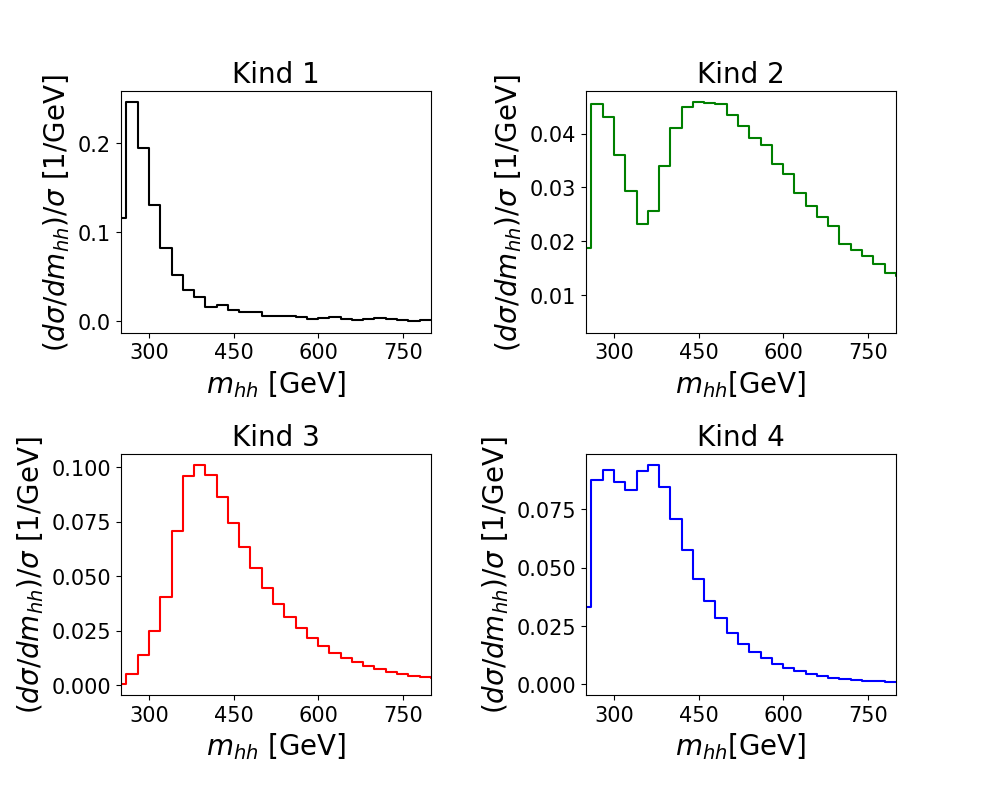
Certainly there is some arbitrariness in the definition of these shapes. For example, shapes of kind 4 would move to kind 1 or 3 for bin widths GeV. However, the other three shape types are quite robust and would be clearly distinguishable experimentally.
Based on the parametrisation in Eq. (5), the normalised differential cross section is computed for a 5-dimensional grid in the coupling parameter space and according to its behaviour is classified into one of the four shape types. For this purpose we wrote a function, called “analyzer” in the following, that checks the slopes of the distribution and puts it into the corresponding class. At this stage the shape classes are mutually exclusive. For each point in the coupling parameter space, we also consider the variations of the result in each bin due to inclusion of the statistical uncertainties on the coefficients . If the shape obtained after these variations belongs to a different kind, we exclude that point from the data set. We find that for shape type 4 about 20% of points fall into this category and are therefore excluded, while for shape type 2 it is about 8%, and for types 1 and 3 it is less than 5%. Scale variations have not been included, as they tend to be rather uniform over the whole range Buchalla:2018yce; Heinrich:2019bkc and therefore would not significantly modify our shape analysis.
2.3 Classification of distributions
Our results for the cross sections at NLO are produced for a centre-of-mass energy of TeV, using PDF4LHC15nlo100pdfas Butterworth:2015oua parton distribution functions interfaced via LHAPDF, along with the corresponding value for . The masses have been set to GeV, GeV and the top quark width has been set to zero.
We study the differential cross section as a function of five anomalous couplings, varying them in the ranges specified below,
| (6) |
The ranges are motivated by current experimental constraints. For we use a smaller range than suggested by experiment in order to focus more on the range where interesting shape features are present. In order to visualise the results, we project out 2-dimensional slices of the 5-dimensional parameter space, fixing the other three couplings to their SM values. This leads to a total of ten configurations. For each of these ten projections we generated a set of parameter pairs. Feeding them through our analyzer we obtain the shape type produced by the given point in the coupling parameter space. The results are shown in Figs. 2–6. The white diamonds denote the Standard Model point in the parameter space. Scale variations are not included, as they are rather uniform over the whole range Buchalla:2018yce; Heinrich:2019bkc and therefore would not modify our shape analysis significantly.

In Fig. 2 we display variations of the top quark Yukawa coupling versus the trilinear Higgs coupling (left) and the effective gluon-Higgs couplings, versus (right). In all the figures where two couplings are varied, the other three couplings are set to their SM values. It can be clearly seen that the shapes of kind 1, i.e. shapes with an enhanced low region (marked in black), are resulting from larger values. The total cross section as a function of is a parabola with a minimum around , while for and the distribution is enhanced in the low region, where the triangle-type contributions dominate. Larger/smaller values of shift this behaviour towards larger/smaller values of because they enhance/decrease the box-type contributions. For shapes of kind 2, i.e double peaks with a separation of more than 100 GeV (green), we find that such a shape can be produced for coupling values which are rather close to the SM values. Shapes of kind 3 (red) are SM-like. They only cover about one quarter of the plane. Shapes of kind 4 (blue) have a double peak separated by less than 100 GeV. For , such structures only occur for negative values of , over the whole allowed range.
Considering variations of versus , shown in the right-hand panel of Fig. 2, we find only shapes of kind 2 (green) and SM-like shapes (red). The existence of kind 2 shapes means that a double peak structure could be produced solely by effective Higgs-gluon couplings, while keeping and at their SM values. However, for the more likely case that deviates only slightly from zero Sirunyan:2018sgc, and so does , these couplings do not distort the SM shape significantly.

Variations of versus and versus are shown in Fig. 3. Varying only and , the shapes remain mainly SM-like. A small area in the plane however contains doubly peaked distributions, which thus can originate from anomalous top-Higgs couplings only, while the trilinear Higgs coupling remains fixed at its SM value.
Turning to versus , displayed in the right-hand panel of Fig. 3, we find that for kind 1 and kind 4 shapes the parameter regions are split into two disconnected parts. While shapes of kind 1 are favoured by large values of , it becomes clear that large values of , also related to triangle-type diagrams, can counterbalance this effect, because the top right corner is not a parameter region producing shapes of kind 1. If both and are large, it is more likely to produce a double peak structure with close-by peaks (kind 4, blue). Further we see that shapes of kind 2 (well separated double peak structure, green) can be produced by values of and which are rather close to the SM values.


Fig. 4 shows variations of versus (left) and versus (right). The parameter space is dominated by SM-like shapes (red), however double peaks can occur as well (green). We also see that acts similarly to in what concerns the shape.

For variations of versus , shown in Fig. 5 (left), all four shape types can occur. The parameter region related to kind 1 (enhanced low , black) is at high values of as expected, and the kind 2 shapes (well separated double peak, green) can be seen as a transition from kind 1 to kind 3. Close-by double peaks (kind 4, blue) however are mostly associated to negative values. Note that a similar pattern can be found in Fig. 2 (left). Variations of versus , shown in Fig. 5 (right), are similar in the overall behaviour, and again show that and have a similar impact on the shape.
Fig. 6 shows variations of versus (left) and versus (right). We observe that SM-like shapes (red) are preferred. However, doubly peaked structures are also possible for values not too far from the SM value (). We also notice the similarity to Fig. 3 (left). The behaviour with respect to is again similar.
Note that in SMEFT, and are related, so this behaviour would necessarily be the case. However we will see later that a shape classification algorithm based on unsupervised learning is able to detect shape differences which distinguish effects of and . An interesting feature is also that kind 1 (black) and kind 4 (blue) shapes appear only when we modify the value of : for shapes of kind 1 never occur, and shapes of kind 4 are very unlikely. Further, the kind 4 shapes tend to point to (moderately) negative values of as long as is close to zero, as can be seen from Figs. 2, 3 and 5.
2.4 Classification of distributions
So far we have studied distributions, assuming that they are very well suited to study the sensitivity to shape changes induced by anomalous couplings. In order to verify that we do not miss out interesting features in the transverse momentum distributions, we also present a study of the distributions, but only at LO, to assess the salient features. The main difference with respect to the case is that in the analysis we could identify only two kinds of clearly distinct shapes: single peak (SM-like, which we denote as ‘ kind 3’) and double peak, with peaks separated by at least 30 GeV (denoted as ‘ kind 2’). Examples of such shapes are shown in Fig. 7.


The parameter spaces leading to singly or doubly peaked shapes are shown in Fig. 8 for the and configurations. The parameter region related to shapes with a well separated double peak (green) is similar to the case, as one can see comparing with Figs. 2 and 3. This indicates that the underlying parameter space leads to similar characteristics for the distributions differential in and , however the distribution is less sensitive than the distribution.
3 Classification and clustering by unsupervised learning
3.1 Unsupervised learning procedure
To assess the bias introduced by the definition of the four shape types, and to find a more flexible classification which can be extended easily to more than four shape types, we approach the classification problem using unsupervised learning techniques. We construct a classification of the shapes of the distribution into distinct types, where we do not predefine what the types should look like. For this purpose we use an autoencoder to find common patterns in the data and thus achieve a compressed representation. The setup is implemented using Keras keras and TensorFlow tensorflow. As input data we use 30 bins of width 20 GeV for the normalised distributions. We train the network based on a set of distributions, retaining 10% for the validation. The encoder architecture, i.e. the part compressing the array information, is composed of two dense layers with 20 nodes and a middle layer with 4 nodes, the latter defining the length of the array containing the compressed information. The decoder architecture, which reconstructs the original array from the compressed one, is composed of two dense layers of 20 nodes and an output layer of the length of the input array. We have also tried other encoder architectures, varying the number of nodes in the layers as well as the number of layers, and found that the results deteriorate for less than three layers. Adding more nodes had the tendency to lead to overfitting.
To test how stable our results are against variations of the training data set and the encoding procedure, and to reduce uncertainties, for example due to overfitting, we produced ten different autoencoder models. For each model we picked random points from the training set for validation to start from different training and validation sets and a different initialization of the weights. We trained the autoencoder for each model over 10000 epochs using Adam Kingma:2014vow as optimizer and the root mean square error to define the loss function. Based on the trained autoencoder we applied the encoder models to the training and validation data to obtain two sets of compressed arrays for each of the ten models. The ten different encoded training data sets are then fed to a classification algorithm, where we employed the KMeans clustering algorithm from scikit-learn scikit, asking for a classification into a given number of clusters. We tested classifications into four to eight clusters.
Asking the KMeans algorithm to find four clusters yielded the shape types shown in Fig. 9, the result of asking for seven clusters is shown in Fig. 10. The curves denote the cluster centres determined by the KMeans algorithm, for each of the ten encoder models, with a colour code as defined in Table 1.
One can see from Figs. 9 and 10 that in the case of clustering into four shape types, cluster 2 contains shapes which vary substantially. In contrast, for seven shape types, the cluster centers obtained from the ten different encoder models are quite similar. Asking for 5–8 clusters we found that seven clusters seemed to be the optimal number to capture distinct shape features, while defining eight clusters did not lead to useful additional features but rather to the tendency to focus on local minima in the clustering space, while neglecting more gobal shape features.


The four clusters shown in Fig. 9 do only partly coincide with the ones defined in Section 2.2. Shapes of kind 1, showing an enhanced region, as well as shapes of kind 3 (SM-like), were clearly identified. Shapes having a double peak were clustered together with shapes showing a shoulder. However, a cluster was formed which was not considered in the predefined types, containing shapes with an enhanced tail.
To combine the results from the ten clustering procedures, we adopted the “majority vote” method, i.e. for each of the ten clustering procedures a given point in the coupling parameter space gets a label (“vote”) corresponding to the cluster it belongs to. The final cluster assigned to that point is the one which collected the largest number of votes.
3.2 Parameter space underlying the clusters
In this section we show how the parameter space relates to the clusters if we ask for four or seven clusters. For each parameter configuration of our 5-dimensional grid, we plot the corresponding cluster type in Fig. 11 and Figs. 13 to 16.
| Cluster | closest predefined type | colour |
|---|---|---|
| 4 clusters | ||
| 1 | kind 1 (enhanced low ) | black |
| 2 | double peak/enhanced tail | magenta |
| 3 | kind 3 (SM-like) | red |
| 4 | kind 4 (close-by double peaks)/shoulder | blue |
| 7 clusters | ||
| 1 | enhanced low | black |
| 2 | enhanced low , slowly falling or shoulder | cyan |
| 3 | enhanced low , second local maximum above | green |
| 4 | SM-like | red |
| 5 | SM-like with enhanced tail | yellow |
| 6 | close-by double peaks or shoulder left | blue |
| 7 | no steep slope at low , enhanced tail | magenta |
The colour codes are shown in Figs. 9 and 10, and are also listed in Table 1. For clusters which are similar to the shape types defined in Section 2.2, we should also find patterns similar to the ones shown in Figs. 2 to 6.


Comparing Fig. 11 (top row) with Fig. 2 (left), both showing variations of versus , we see that kind 1 shapes (black) are clearly identified. However, for both four and seven clusters the area for SM-like shapes got smaller, as the clustering algorithm also identifies features which were not considered in the predefined shapes. For example, the clustering into four clusters identifies shapes which are almost SM-like but have an enhanced tail (magenta), and the clustering into seven clusters in addition identifies shapes which are almost SM-like but have a shoulder (blue). Certainly we could have defined such features in our analyzer as well, but it is not that easy to define where the tail starts and what exactly should be considered as “enhanced”. Further, the figure clearly shows that small variations of can easily distort the SM-like shape, while the shape is more robust against variations of . Fig. 11 (bottom row) shows versus . We again see that variations and mostly produce SM-like shapes. Why this is so can be understood from the behaviour of the coefficients in eq. (5) which are relevant in these cases. For Fig. 11 (top row), only the coefficients and are relevant. As and have opposite signs and a different peak location, this can generate a rich shape structure. For Fig. 11 (bottom row), the coefficients and are relevant in addition to and . being the coefficient of , it is dominant except for very small values of and leads to a SM-like shape. We also observe that has the tendency to enhance the total cross section, such that only a relatively small slice in is left after considering the bounds on the total cross section.


Fig. 13 (top row) shows versus , where we see that the interplay between and can lead to all shape types. Comparing Fig. 13 (bottom row) with Fig. 2 (right), showing variations of versus , we observe that the unsupervised learning algorithm with seven clusters distinguishes four shape types, showing that large values of and favour shapes with an enhanced tail (magenta) or/and a double peak (green), while negative values favour a shoulder on the left of the peak (blue). The limits on the total cross section do not exclude any parameter range in this panel.


A behaviour similar to the one in Fig. 11 can be seen in Fig. 14: as varies the disribution goes through various shape types, while variations of and affect the shapes to less extent. Fig. 14 also shows that a positive value has the tendency to enhance the tail of the distribution.


Fig. 15 shows versus (top) and versus (bottom). Compared to Fig. 6, the clustering into both four and seven clusters shows a better discrimination power between SM-like shapes and small deviations, for example due to an enhanced tail. We again see that has a larger impact on the total cross section than or .
Fig. 16, showing the and parameter planes, can be compared to Fig. 4. Again, both the case of four and of seven clusters indicates that the unsupervised learning algorithm is able to distinguish better subtle influences on the shape than our method based on humanly classified shapes.
In Fig. 17, we compare results of our shape analysis produced with LO and NLO input data. We observe that NLO corrections can change the shape considerably and therefore are important for a shape analysis.

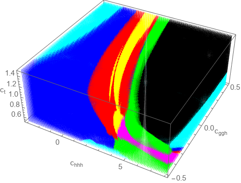
The results above have shown that the parameters and have the largest influence on the shape. In SMEFT, is suppressed compared to by one order of the large new physics scale DiMicco:2019ngk. Furthermore, SMEFT imposes the relation (4) between and . Using this relation and imposing that amounts to 5% of , we obtain a 3-dimensional parameter space simulating the SMEFT situation, which is visualized in Fig. 18.
3.3 Identification of benchmark points
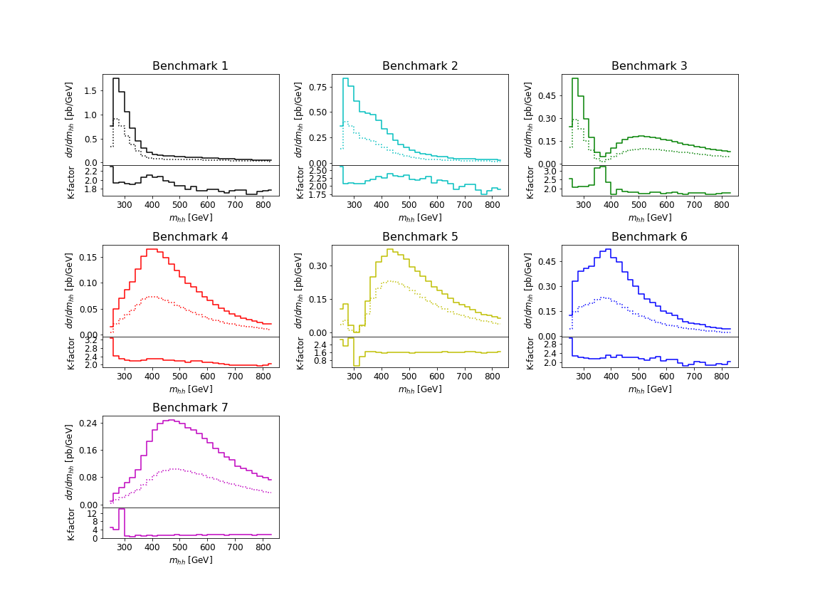
The determination of the cluster centres allows to identify NLO benchmark points which should be representative for each characteristic shape. As the cluster centres determined by the KMeans algorithm do not necessarily correspond to grid points of our input grids in parameter space, and as we work with normalised distributions to find the cluster centres, we determine the benchmark points based on the following procedure
- 1.
We identify the grid point in parameter space corresponding to a curve which is closest to the cluster centre, where the distance measure is the bin-wise geometric distance to the cluster center of the encoded distribution.
- 2.
If the corresponding total cross section exceeds the limit of Aad:2019uzh, we proceed to the curve which is the next-closest to the cluster center.
- 3.
If several curves determined this way have an identical distance measure, we choose the one where the value of is closer to the SM value (anticipating that the top-Higgs Yukawa coupling will be constrained increasingly well from other processes).
- 4.
If after this procedure there are still several curves satisfying these criteria, from these curves we pick the one closest to the cluster center according to the Kullback–Leibler Kullback-Leibler distance measure, applied to the normalised distributions.
Following this procedure we find the benchmark points listed in Table 2. In Fig. 19 we show the distributions corresponding to these benchmark points, at LO as well as at NLO.
| benchmark | [pb] | K-factor | ratio to SM | |||||
| 1 | 0.94 | 3.94 | - | 0.5 | 182.50 5.11 | 1.93 | 6.64 | |
| 2 | 0.61 | 6.84 | 0.0 | - | 135.63 4.27 | 2.16 | 4.93 | |
| 3 | 1.05 | 2.21 | - | 0.5 | 0.5 | 109.24 2.65 | 1.86 | 3.97 |
| 4 | 0.61 | 2.79 | -0.5 | 50.44 1.53 | 2.16 | 1.83 | ||
| 5 | 1.17 | 3.95 | - | -0.5 | 116.68 6.25 | 1.63 | 4.24 | |
| 6 | 0.83 | 5.68 | -0.5 | 145.37 8.25 | 2.19 | 5.29 | ||
| 7 | 0.94 | -0.10 | 1 | - | 96.69 1.45 | 2.29 | 3.52 |
4 Conclusions
The aim of this work was to provide more insight how certain configurations of anomalous couplings in the Higgs sector lead to a corresponding characteristic shape of the Higgs boson pair invariant mass distribution. For this purpose we employed the Lagrangian relevant to Higgs boson pair production as given in a non-linear Effective Field Theory framework, which contains five (potentially) anomalous couplings Buchalla:2018yce. We produced data for the Higgs boson pair invariant mass distribution, based on a calculation which includes the NLO QCD corrections with full top quark mass dependence, varying all five coupling parameters by finite steps, thus producing a dense grid of data. Then we defined four characteristic shape types for the distribution and visualised the parameter space leading to these shape types. To this aim we projected onto all possible two-dimensional slices of the parameter space, keeping the remaining parameters at their Standard Model values. We also considered distributions for a shape analysis, however we found that the distribution is more sensitive to shape changes induced by anomalous couplings.
Further, we tested an unsupervised learning approach to classify shapes. We produced distributions, trained a neural network based on an autoencoder to extract common shape features and tried to find the number of shape clusters which optimally catches different shape characteristics. Our study demonstrated that some shape features, like an enhanced tail or a shoulder in the distribution, were caught very well by this procedure, and provided more insight about the underlying parameter space leading to such features than the analysis based on predefined shape classes. While machine learning is not essential to define shape clusters, it has the advantage of being easily extendible to a different number of shape types, different binnings or other observables, and of minimising the human bias compared to other shape analysis methods.
The shape analysis revealed that the Standard-Model-like shape is quite stable against variations of and , as long as , while deviations of from the SM value show a rich shape changing pattern. We also found that small deviations of from zero are very likely to produce a doubly peaked structure in the distribution, while SM-like shapes dominate again as moves further away from zero. However, as leads to a rather fast increase of the total cross section, the shape analysis in combination with the limits on the total cross section allows to put constraints on . This is an interesting feature because, in contrast to and , cannot be constrained directly from single Higgs boson processes. Further, an enhanced tail or a shoulder of the distribution are likely to be produced by nonzero values of , however the influence of the effective Higgs-gluon couplings on the shape is milder than the one of and .
We also provide seven benchmark points, based on the full NLO calculation and taking into account current experimental constraints, which lead to the characteristic shapes as represented by our cluster centers.
The method can also be applied to other processes where anomalous couplings introduce characteristic shape changes to differential cross sections, and it can be extended to consider more than one distribution simultaneously.
Acknowledgements
We would like to thank Gerhard Buchalla, Alejandro Celis, Long Chen, Victor Diaz, Stephan Jahn, Stephen P. Jones, Matthias Kerner, Gionata Luisoni, Ludovic Scyboz and Johannes Schlenk for collaboration on the HH code, for useful discussions and for valuable comments on the manuscript. This research was supported in part by the COST Action CA16201 (‘Particleface’) of the European Union.
References
- (1) ATLAS collaboration, G. Aad et al., Combination of searches for Higgs boson pairs in collisions at 13 TeV with the ATLAS detector, Phys. Lett. B800 (2020) 135103 [1906.02025].
- (2) CMS collaboration, A. M. Sirunyan et al., Combination of searches for Higgs boson pair production in proton-proton collisions at 13 TeV, Phys. Rev. Lett. 122 (2019) 121803 [1811.09689].
- (3) M. McCullough, An Indirect Model-Dependent Probe of the Higgs Self-Coupling, Phys. Rev. D90 (2014) 015001 [1312.3322].
- (4) M. Gorbahn and U. Haisch, Indirect probes of the trilinear Higgs coupling: and , JHEP 10 (2016) 094 [1607.03773].
- (5) G. Degrassi, P. P. Giardino, F. Maltoni and D. Pagani, Probing the Higgs self coupling via single Higgs production at the LHC, JHEP 12 (2016) 080 [1607.04251].
- (6) W. Bizon, M. Gorbahn, U. Haisch and G. Zanderighi, Constraints on the trilinear Higgs coupling from vector boson fusion and associated Higgs production at the LHC, JHEP 07 (2017) 083 [1610.05771].
- (7) F. Maltoni, D. Pagani, A. Shivaji and X. Zhao, Trilinear Higgs coupling determination via single-Higgs differential measurements at the LHC, Eur. Phys. J. C77 (2017) 887 [1709.08649].
- (8) G. D. Kribs, A. Maier, H. Rzehak, M. Spannowsky and P. Waite, Electroweak oblique parameters as a probe of the trilinear Higgs boson self-interaction, Phys. Rev. D95 (2017) 093004 [1702.07678].
- (9) G. Degrassi, M. Fedele and P. P. Giardino, Constraints on the trilinear Higgs self coupling from precision observables, JHEP 04 (2017) 155 [1702.01737].
- (10) J. Nakamura and A. Shivaji, Direct measurement of the Higgs self-coupling in , Phys. Lett. B797 (2019) 134821 [1812.01576].
- (11) W. Kilian, S. Sun, Q.-S. Yan, X. Zhao and Z. Zhao, Multi-Higgs Production and Unitarity in Vector-Boson Fusion at Future Hadron Colliders, 1808.05534.
- (12) F. Maltoni, D. Pagani and X. Zhao, Constraining the Higgs self-couplings at e+e- colliders, JHEP 07 (2018) 087 [1802.07616].
- (13) E. Vryonidou and C. Zhang, Dimension-six electroweak top-loop effects in Higgs production and decay, JHEP 08 (2018) 036 [1804.09766].
- (14) M. Gorbahn and U. Haisch, Two-loop amplitudes for Higgs plus jet production involving a modified trilinear Higgs coupling, JHEP 04 (2019) 062 [1902.05480].
- (15) ATLAS collaboration, Constraint of the Higgs boson self-coupling from Higgs boson differential production and decay measurements, Tech. Rep. ATL-PHYS-PUB-2019-009, CERN, Geneva, Mar, 2019.
- (16) ATLAS collaboration, Constraints on the Higgs boson self-coupling from the combination of single-Higgs and double-Higgs production analyses performed with the ATLAS experiment, Tech. Rep. ATL-PHYS-PUB-2019-049, CERN, Geneva, Oct, 2019.
- (17) W. Bizon, U. Haisch and L. Rottoli, Constraints on the quartic Higgs self-coupling from double-Higgs production at future hadron colliders, JHEP 10 (2019) 267 [1810.04665].
- (18) S. Borowka, C. Duhr, F. Maltoni, D. Pagani, A. Shivaji and X. Zhao, Probing the scalar potential via double Higgs boson production at hadron colliders, JHEP 04 (2019) 016 [1811.12366].
- (19) A. Falkowski and R. Rattazzi, Which EFT, JHEP 10 (2019) 255 [1902.05936].
- (20) S. Chang and M. A. Luty, The Higgs Trilinear Coupling and the Scale of New Physics, 1902.05556.
- (21) L. Di Luzio, R. Gröber and M. Spannowsky, Maxi-sizing the trilinear Higgs self-coupling: how large could it be?, Eur. Phys. J. C77 (2017) 788 [1704.02311].
- (22) S. Di Vita, C. Grojean, G. Panico, M. Riembau and T. Vantalon, A global view on the Higgs self-coupling, JHEP 09 (2017) 069 [1704.01953].
- (23) J. Braathen and S. Kanemura, On two-loop corrections to the Higgs trilinear coupling in models with extended scalar sectors, Phys. Lett. B796 (2019) 38 [1903.05417].
- (24) P. Basler, S. Dawson, C. Englert and M. Mühlleitner, Showcasing HH production: Benchmarks for the LHC and HL-LHC, Phys. Rev. D99 (2019) 055048 [1812.03542].
- (25) K. S. Babu and S. Jana, Enhanced Di-Higgs Production in the Two Higgs Doublet Model, JHEP 02 (2019) 193 [1812.11943].
- (26) A. Adhikary, S. Banerjee, R. K. Barman, B. Bhattacherjee and S. Niyogi, Revisiting the non-resonant Higgs pair production at the HL-LHC, JHEP 07 (2018) 116 [1712.05346].
- (27) I. M. Lewis and M. Sullivan, Benchmarks for Double Higgs Production in the Singlet Extended Standard Model at the LHC, Phys. Rev. D96 (2017) 035037 [1701.08774].
- (28) S. Dawson, C. Englert and T. Plehn, Higgs Physics: It ain’t over till it’s over, Phys. Rept. 816 (2019) 1 [1808.01324].
- (29) M. Cepeda et al., Report from Working Group 2, CERN Yellow Rep. Monogr. 7 (2019) 221 [1902.00134].
- (30) J. Alison et al., Higgs Boson Pair Production at Colliders: Status and Perspectives, in Double Higgs Production at Colliders Batavia, IL, USA, September 4, 2018-9, 2019 (B. Di Micco, M. Gouzevitch, J. Mazzitelli and C. Vernieri, eds.), 2019, 1910.00012, https://lss.fnal.gov/archive/2019/conf/fermilab-conf-19-468-e-t.pdf.
- (31) O. J. P. Eboli, G. C. Marques, S. F. Novaes and A. A. Natale, Twin Higgs Boson Production, Phys. Lett. B197 (1987) 269.
- (32) E. W. N. Glover and J. J. van der Bij, Higgs Boson Pair Production via Gluon Fusion, Nucl. Phys. B309 (1988) 282.
- (33) T. Plehn, M. Spira and P. M. Zerwas, Pair production of neutral Higgs particles in gluon-gluon collisions, Nucl. Phys. B479 (1996) 46 [hep-ph/9603205].
- (34) S. Dawson, S. Dittmaier and M. Spira, Neutral Higgs boson pair production at hadron colliders: QCD corrections, Phys. Rev. D58 (1998) 115012 [hep-ph/9805244].
- (35) F. Maltoni, E. Vryonidou and M. Zaro, Top-quark mass effects in double and triple Higgs production in gluon-gluon fusion at NLO, JHEP 11 (2014) 079 [1408.6542].
- (36) S. Borowka, N. Greiner, G. Heinrich, S. P. Jones, M. Kerner, J. Schlenk et al., Higgs Boson Pair Production in Gluon Fusion at Next-to-Leading Order with Full Top-Quark Mass Dependence, Phys. Rev. Lett. 117 (2016) 012001 [1604.06447].
- (37) S. Borowka, N. Greiner, G. Heinrich, S. P. Jones, M. Kerner, J. Schlenk et al., Full top quark mass dependence in Higgs boson pair production at NLO, JHEP 10 (2016) 107 [1608.04798].
- (38) J. Baglio, F. Campanario, S. Glaus, M. Mühlleitner, M. Spira and J. Streicher, Gluon fusion into Higgs pairs at NLO QCD and the top mass scheme, Eur. Phys. J. C79 (2019) 459 [1811.05692].
- (39) J. Baglio, F. Campanario, S. Glaus, M. M. Mühlleitner, J. Ronca, M. Spira et al., Higgs-Pair Production via Gluon Fusion at Hadron Colliders: NLO QCD Corrections, 2003.03227.
- (40) G. Heinrich, S. P. Jones, M. Kerner, G. Luisoni and E. Vryonidou, NLO predictions for Higgs boson pair production with full top quark mass dependence matched to parton showers, JHEP 08 (2017) 088 [1703.09252].
- (41) S. Jones and S. Kuttimalai, Parton Shower and NLO-Matching uncertainties in Higgs Boson Pair Production, JHEP 02 (2018) 176 [1711.03319].
- (42) G. Heinrich, S. P. Jones, M. Kerner, G. Luisoni and L. Scyboz, Probing the trilinear Higgs boson coupling in di-Higgs production at NLO QCD including parton shower effects, JHEP 06 (2019) 066 [1903.08137].
- (43) D. de Florian and J. Mazzitelli, Two-loop virtual corrections to Higgs pair production, Phys. Lett. B724 (2013) 306 [1305.5206].
- (44) D. de Florian and J. Mazzitelli, Higgs Boson Pair Production at Next-to-Next-to-Leading Order in QCD, Phys. Rev. Lett. 111 (2013) 201801 [1309.6594].
- (45) J. Grigo, K. Melnikov and M. Steinhauser, Virtual corrections to Higgs boson pair production in the large top quark mass limit, Nucl. Phys. B888 (2014) 17 [1408.2422].
- (46) J. Grigo, J. Hoff and M. Steinhauser, Higgs boson pair production: top quark mass effects at NLO and NNLO, Nucl. Phys. B900 (2015) 412 [1508.00909].
- (47) D. de Florian, M. Grazzini, C. Hanga, S. Kallweit, J. M. Lindert, P. Maierhöfer et al., Differential Higgs Boson Pair Production at Next-to-Next-to-Leading Order in QCD, JHEP 09 (2016) 151 [1606.09519].
- (48) M. Grazzini, G. Heinrich, S. Jones, S. Kallweit, M. Kerner, J. M. Lindert et al., Higgs boson pair production at NNLO with top quark mass effects, JHEP 05 (2018) 059 [1803.02463].
- (49) D. De Florian and J. Mazzitelli, Soft gluon resummation for Higgs boson pair production including finite Mt effects, JHEP 08 (2018) 156 [1807.03704].
- (50) R. Gröber, A. Maier and T. Rauh, Reconstruction of top-quark mass effects in Higgs pair production and other gluon-fusion processes, JHEP 03 (2018) 020 [1709.07799].
- (51) R. Bonciani, G. Degrassi, P. P. Giardino and R. Gröber, Analytical Method for Next-to-Leading-Order QCD Corrections to Double-Higgs Production, Phys. Rev. Lett. 121 (2018) 162003 [1806.11564].
- (52) X. Xu and L. L. Yang, Towards a new approximation for pair-production and associated-production of the Higgs boson, JHEP 01 (2019) 211 [1810.12002].
- (53) J. Davies, G. Mishima, M. Steinhauser and D. Wellmann, Double-Higgs boson production in the high-energy limit: planar master integrals, JHEP 03 (2018) 048 [1801.09696].
- (54) J. Davies, F. Herren, G. Mishima and M. Steinhauser, Real-virtual corrections to Higgs boson pair production at NNLO: three closed top quark loops, JHEP 05 (2019) 157 [1904.11998].
- (55) J. Davies, G. Mishima, M. Steinhauser and D. Wellmann, Double Higgs boson production at NLO in the high-energy limit: complete analytic results, JHEP 01 (2019) 176 [1811.05489].
- (56) J. Davies, G. Heinrich, S. P. Jones, M. Kerner, G. Mishima, M. Steinhauser et al., Double Higgs boson production at NLO: combining the exact numerical result and high-energy expansion, JHEP 11 (2019) 024 [1907.06408].
- (57) R. Contino, M. Ghezzi, M. Moretti, G. Panico, F. Piccinini and A. Wulzer, Anomalous Couplings in Double Higgs Production, JHEP 08 (2012) 154 [1205.5444].
- (58) F. Goertz, A. Papaefstathiou, L. L. Yang and J. Zurita, Higgs boson pair production in the D=6 extension of the SM, JHEP 04 (2015) 167 [1410.3471].
- (59) C.-R. Chen and I. Low, Double take on new physics in double Higgs boson production, Phys. Rev. D90 (2014) 013018 [1405.7040].
- (60) A. Azatov, R. Contino, G. Panico and M. Son, Effective field theory analysis of double Higgs boson production via gluon fusion, Phys. Rev. D92 (2015) 035001 [1502.00539].
- (61) S. Dawson, A. Ismail and I. Low, What’s in the loop? The anatomy of double Higgs production, Phys. Rev. D91 (2015) 115008 [1504.05596].
- (62) A. Carvalho, M. Dall’Osso, T. Dorigo, F. Goertz, C. A. Gottardo and M. Tosi, Higgs Pair Production: Choosing Benchmarks With Cluster Analysis, JHEP 04 (2016) 126 [1507.02245].
- (63) Q.-H. Cao, B. Yan, D.-M. Zhang and H. Zhang, Resolving the Degeneracy in Single Higgs Production with Higgs Pair Production, Phys. Lett. B752 (2016) 285 [1508.06512].
- (64) Q.-H. Cao, G. Li, B. Yan, D.-M. Zhang and H. Zhang, Double Higgs production at the 14 TeV LHC and a 100 TeV collider, Phys. Rev. D96 (2017) 095031 [1611.09336].
- (65) J. de Blas, O. Eberhardt and C. Krause, Current and Future Constraints on Higgs Couplings in the Nonlinear Effective Theory, JHEP 07 (2018) 048 [1803.00939].
- (66) R. Gröber, M. Mühlleitner, M. Spira and J. Streicher, NLO QCD Corrections to Higgs Pair Production including Dimension-6 Operators, JHEP 09 (2015) 092 [1504.06577].
- (67) R. Gröber, M. Mühlleitner and M. Spira, Signs of Composite Higgs Pair Production at Next-to-Leading Order, JHEP 06 (2016) 080 [1602.05851].
- (68) F. Maltoni, E. Vryonidou and C. Zhang, Higgs production in association with a top-antitop pair in the Standard Model Effective Field Theory at NLO in QCD, JHEP 10 (2016) 123 [1607.05330].
- (69) R. Gröber, M. Mühlleitner and M. Spira, Higgs Pair Production at NLO QCD for CP-violating Higgs Sectors, Nucl. Phys. B925 (2017) 1 [1705.05314].
- (70) D. de Florian, I. Fabre and J. Mazzitelli, Higgs boson pair production at NNLO in QCD including dimension 6 operators, JHEP 10 (2017) 215 [1704.05700].
- (71) G. Buchalla, M. Capozi, A. Celis, G. Heinrich and L. Scyboz, Higgs boson pair production in non-linear Effective Field Theory with full -dependence at NLO QCD, JHEP 09 (2018) 057 [1806.05162].
- (72) A. Carvalho, M. Dall’Osso, P. De Castro Manzano, T. Dorigo, F. Goertz, M. Gouzevich et al., Analytical parametrization and shape classification of anomalous HH production in the EFT approach, 1608.06578.
- (73) A. Carvalho, F. Goertz, K. Mimasu, M. Gouzevitch and A. Aggarwal, On the reinterpretation of non-resonant searches for Higgs boson pairs, 1710.08261.
- (74) https://www.scikit-learn.org.
- (75) L. de Oliveira, M. Kagan, L. Mackey, B. Nachman and A. Schwartzman, Jet-images – deep learning edition, JHEP 07 (2016) 069 [1511.05190].
- (76) J. Brehmer, K. Cranmer, F. Kling and T. Plehn, Better Higgs boson measurements through information geometry, Phys. Rev. D95 (2017) 073002 [1612.05261].
- (77) J. Brehmer, K. Cranmer, G. Louppe and J. Pavez, Constraining Effective Field Theories with Machine Learning, Phys. Rev. Lett. 121 (2018) 111801 [1805.00013].
- (78) J. Brehmer, K. Cranmer, G. Louppe and J. Pavez, A Guide to Constraining Effective Field Theories with Machine Learning, Phys. Rev. D98 (2018) 052004 [1805.00020].
- (79) D. Guest, J. Collado, P. Baldi, S.-C. Hsu, G. Urban and D. Whiteson, Jet Flavor Classification in High-Energy Physics with Deep Neural Networks, Phys. Rev. D94 (2016) 112002 [1607.08633].
- (80) G. Kasieczka, T. Plehn, M. Russell and T. Schell, Deep-learning Top Taggers or The End of QCD?, JHEP 05 (2017) 006 [1701.08784].
- (81) K. Datta and A. J. Larkoski, Novel Jet Observables from Machine Learning, JHEP 03 (2018) 086 [1710.01305].
- (82) G. Louppe, K. Cho, C. Becot and K. Cranmer, QCD-Aware Recursive Neural Networks for Jet Physics, JHEP 01 (2019) 057 [1702.00748].
- (83) A. J. Larkoski, I. Moult and B. Nachman, Jet Substructure at the Large Hadron Collider: A Review of Recent Advances in Theory and Machine Learning, 1709.04464.
- (84) S. Macaluso and D. Shih, Pulling Out All the Tops with Computer Vision and Deep Learning, JHEP 10 (2018) 121 [1803.00107].
- (85) S. Bollweg, M. Haußmann, G. Kasieczka, M. Luchmann, T. Plehn and J. Thompson, Deep-Learning Jets with Uncertainties and More, SciPost Phys. 8 (2020) 006 [1904.10004].
- (86) A. Butter et al., The Machine Learning Landscape of Top Taggers, SciPost Phys. 7 (2019) 014 [1902.09914].
- (87) A. Butter, T. Plehn and R. Winterhalder, How to GAN LHC Events, SciPost Phys. 7 (2019) 075 [1907.03764].
- (88) E. A. Moreno, O. Cerri, J. M. Duarte, H. B. Newman, T. Q. Nguyen, A. Periwal et al., JEDI-net: a jet identification algorithm based on interaction networks, Eur. Phys. J. C80 (2020) 58 [1908.05318].
- (89) Y.-C. J. Chen, C.-W. Chiang, G. Cottin and D. Shih, Boosted Tagging with Jet Charge and Deep Learning, 1908.08256.
- (90) J. Chang, K. Cheung, J. S. Lee and J. Park, Probing the trilinear Higgs boson self-coupling at the high-luminosity LHC via multivariate analysis, Phys. Rev. D101 (2020) 016004 [1908.00753].
- (91) S. Carrazza and J. Cruz-Martinez, Towards a new generation of parton densities with deep learning models, Eur. Phys. J. C79 (2019) 676 [1907.05075].
- (92) J. Hajer, Y.-Y. Li, T. Liu and H. Wang, Novelty Detection Meets Collider Physics, 1807.10261.
- (93) A. De Simone and T. Jacques, Guiding New Physics Searches with Unsupervised Learning, Eur. Phys. J. C79 (2019) 289 [1807.06038].
- (94) A. Andreassen, I. Feige, C. Frye and M. D. Schwartz, JUNIPR: a Framework for Unsupervised Machine Learning in Particle Physics, Eur. Phys. J. C79 (2019) 102 [1804.09720].
- (95) R. T. D’Agnolo and A. Wulzer, Learning New Physics from a Machine, Phys. Rev. D99 (2019) 015014 [1806.02350].
- (96) S. Chang, T. Cohen and B. Ostdiek, What is the Machine Learning?, Phys. Rev. D97 (2018) 056009 [1709.10106].
- (97) C. Englert, P. Galler, P. Harris and M. Spannowsky, Machine Learning Uncertainties with Adversarial Neural Networks, Eur. Phys. J. C79 (2019) 4 [1807.08763].
- (98) A. Blance, M. Spannowsky and P. Waite, Adversarially-trained autoencoders for robust unsupervised new physics searches, JHEP 10 (2019) 047 [1905.10384].
- (99) J. Brehmer, S. Dawson, S. Homiller, F. Kling and T. Plehn, Benchmarking simplified template cross sections in production, JHEP 11 (2019) 034 [1908.06980].
- (100) F. F. Freitas, C. K. Khosa and V. Sanz, Exploring the standard model EFT in VH production with machine learning, Phys. Rev. D100 (2019) 035040 [1902.05803].
- (101) G. Buchalla, O. Cata, A. Celis and C. Krause, Note on Anomalous Higgs-Boson Couplings in Effective Field Theory, Phys. Lett. B750 (2015) 298 [1504.01707].
- (102) L. Berthier and M. Trott, Towards consistent Electroweak Precision Data constraints in the SMEFT, JHEP 05 (2015) 024 [1502.02570].
- (103) I. Brivio, Y. Jiang and M. Trott, The SMEFTsim package, theory and tools, JHEP 12 (2017) 070 [1709.06492].
- (104) C. Arzt, M. B. Einhorn and J. Wudka, Patterns of deviation from the standard model, Nucl. Phys. B433 (1995) 41 [hep-ph/9405214].
- (105) J. Butterworth et al., PDF4LHC recommendations for LHC Run II, J. Phys. G43 (2016) 023001 [1510.03865].
- (106) CMS collaboration, A. M. Sirunyan et al., Measurement and interpretation of differential cross sections for Higgs boson production at 13 TeV, Phys. Lett. B792 (2019) 369 [1812.06504].
- (107) https://keras.io.
- (108) https://www.tensorflow.org.
- (109) D. P. Kingma and J. Ba, Adam: A Method for Stochastic Optimization, 1412.6980.
- (110) S. Kullback, Information Theory and Statistics. John Wiley & Sons. Republished by Dover Publications, 1978.