跳到论文正文
W Papers独立论文阅读器 arXiv:1908.08901 论文正文 计算阅读时间 · 0%
引用这篇论文根据当前论文元数据生成,正式投稿前建议核对。


License: arXiv.org perpetual non-exclusive license
arXiv:1908.08901v1 [math.NA] 23 Aug 2019

Application of Randomized Quadrature Formulas
to the Finite Element Method
for Elliptic Equations

Raphael Kruse Address: Raphael Kruse
Institut für Mathematik
Technische Universität Berlin
Straße des 17. Juni 136
DE-10623 Berlin
Germany
Email address: kruse@math.tu-berlin.de
, Nick Polydorides Address: Nick Polydorides
School of Engineering
University of Edinburgh
Edinburgh, EH9 3FB
UK; The Alan Turing Institute, London, UK
Email address: n.polydorides@ed.ac.uk
and Yue Wu Address: Yue Wu
Mathematical Institute
University of Oxford
Oxford, OX2 6GG
UK
Email address: yue.wu@maths.ox.ac.uk
Abstract.

The implementation of the finite element method for linear elliptic equations requires to assemble the stiffness matrix and the load vector. In general, the entries of this matrix-vector system are not known explicitly but need to be approximated by quadrature rules. If the coefficient functions of the differential operator or the forcing term are irregular, then standard quadrature formulas, such as the barycentric quadrature rule, may not be reliable. In this paper we investigate the application of two randomized quadrature formulas to the finite element method for such elliptic boundary value problems with irregular coefficient functions. We give a detailed error analysis of these methods, discuss their implementation, and demonstrate their capabilities in several numerical experiments.

Key words and phrases: 
finite element method, Monte Carlo method, quadrature, elliptic equations
2010 Mathematics Subject Classification
65C05, 65D32, 65N15, 65N30

1. Introduction

Let 𝒟⊂ℝ2{\mathcal{D}}\subset{\mathbb{R}}^{2} be a convex, bounded, and polygonal domain. We consider a linear elliptic boundary value problem of the following form: Find a mapping u:𝒟→ℝu\colon{\mathcal{D}}\to{\mathbb{R}} such that

(1) {−div(σ∇u)=f, in ​𝒟,u=0, on ​∂𝒟,\displaystyle\begin{cases}-\mathrm{div}\big(\sigma\nabla u\big)=f,&\text{ in }{\mathcal{D}},\\ u=0,&\text{ on }\partial{\mathcal{D}},\end{cases}

where σ,f:𝒟→ℝ\sigma,f\colon{\mathcal{D}}\to{\mathbb{R}} are given coefficient functions with σ⁡(x)≥σ0>0\sigma(x)\geq\sigma_{0}>0 for all x∈𝒟x\in{\mathcal{D}}. Provided σ\sigma is globally bounded and ff is square-integrable, it is well-known that (1) admits a unique solution u∈H01​(𝒟)u\in H^{1}_{0}({\mathcal{D}}) in the weak sense satisfying

(2) ∫𝒟σ(x)∇u(x)⋅∇v(x)dx=∫𝒟f(x)v(x)dx\displaystyle\int_{\mathcal{D}}\sigma(x)\nabla u(x)\cdot\nabla v(x)\,\mathrm{d}x=\int_{\mathcal{D}}f(x)v(x)\,\mathrm{d}x

for all v∈H01​(𝒟)v\in H^{1}_{0}({\mathcal{D}}). Here, we denote by H01​(𝒟)H^{1}_{0}({\mathcal{D}}) the Sobolev space of weakly differentiable and square-integrable functions which (in some sense) satisfy the homogeneous Dirichlet boundary condition. In Section 2 we provide more details on the function spaces used throughout this paper. We also refer, for instance, to [5, Chapters 8–9] or [11, Chapter 6] for an introduction to the variational formulation of elliptic boundary value problems of the form (1).

Elliptic equations such as (1) appear in many applications, e.g., in mechanical engineering and physics. It is also an intensively studied problem to introduce the Galerkin finite element method as found in many text books in numerical analysis, e.g. [4, 27, 28, 36]. In the same spirit, we use (1) as a model problem to demonstrate the applicability of randomized quadrature formulas to the finite element method.

To this end, we consider a family (𝒯h)h∈(0,1](\mathcal{T}_{h})_{h\in(0,1]} of finite subdivisions of the polygonal domain 𝒟⊂ℝ2{\mathcal{D}}\subset{\mathbb{R}}^{2} into triangles. Hereby, the parameter h∈(0,1]h\in(0,1] denotes the maximal edge length of the elements in 𝒯h\mathcal{T}_{h}. For every partition 𝒯h\mathcal{T}_{h} we define Sh⊂H01​(𝒟)S_{h}\subset H^{1}_{0}({\mathcal{D}}) as the associated finite element space consisting of piecewise linear functions.

Then, we obtain an approximation of the exact solution to the boundary value problem (1) by solving the following finite dimensional problem: For h∈(0,1]h\in(0,1] find uh∈Shu_{h}\in S_{h} satisfying

(3) ∫𝒟σ(x)∇uh(x)⋅∇vh(x)dx=∫𝒟f(x)vh(x)dx\displaystyle\int_{\mathcal{D}}\sigma(x)\nabla u_{h}(x)\cdot\nabla v_{h}(x)\,\mathrm{d}x=\int_{\mathcal{D}}f(x)v_{h}(x)\,\mathrm{d}x

for all vh∈Shv_{h}\in S_{h}. For the practical computation of the approximation uh∈Shu_{h}\in S_{h}, it is then convenient to rewrite (3) as a system of linear equations. More precisely, let (φj)j=1Nh(\varphi_{j})_{j=1}^{N_{h}} be a basis of ShS_{h}, where Nh=dim(Sh)N_{h}=\dim(S_{h}) denotes the number of degrees of freedom. Then, we have the representation

uh=∑j=1Nhuj​φj,\displaystyle u_{h}=\sum_{j=1}^{N_{h}}u_{j}\varphi_{j},

where the entries of the vector 𝐮=[u1,…,uNh]⊤∈ℝNh\mathbf{u}=[u_{1},\ldots,u_{N_{h}}]^{\top}\in{\mathbb{R}}^{N_{h}} are yet to be determined. After inserting this representation of uhu_{h} into the finite dimensional problem (3) and by testing with all basis functions (φj)j=1Nh(\varphi_{j})_{j=1}^{N_{h}} we arrive at a system of linear equations. In matrix-vector form this system is written as

(4) Ah​𝐮=fh,\displaystyle A_{h}\mathbf{u}=f_{h},

where the stiffness matrix Ah∈ℝNh×NhA_{h}\in{\mathbb{R}}^{N_{h}\times N_{h}} is given by

[Ah]i,j=∫𝒟σ(x)∇φi(x)⋅∇φj(x)dx\displaystyle[A_{h}]_{i,j}=\int_{\mathcal{D}}\sigma(x)\nabla\varphi_{i}(x)\cdot\nabla\varphi_{j}(x)\,\mathrm{d}x

for all i,j∈{1,…,Nh}i,j\in\{1,\ldots,N_{h}\}. Moreover, the load vector fh∈ℝNhf_{h}\in{\mathbb{R}}^{N_{h}} has the entries

(5) [fh]i=∫𝒟f⁡(x)​φi​(x)​𝑑x,i∈{1,…,Nh}.\displaystyle[f_{h}]_{i}=\int_{\mathcal{D}}f(x)\varphi_{i}(x)\,\mathrm{d}x,\quad i\in\{1,\ldots,N_{h}\}.

If, on the one hand, the entries of AhA_{h} and fhf_{h} are known explicitly, it is straight-forward to use standard solvers for the linear system (4) in order to determine 𝐮∈ℝNh\mathbf{u}\in{\mathbb{R}}^{N_{h}} and, hence, uh∈Shu_{h}\in S_{h} numerically. For instance, we refer to the monograph [17] for an overview of suitable solvers.

On the other hand, for general σ∈L∞​(𝒟)\sigma\in L^{\infty}({\mathcal{D}}) and f∈L2​(𝒟)f\in L^{2}({\mathcal{D}}), the entries of the stiffness matrix and the load vector are often not computable explicitly. Such irregular coefficients often appear in problems in uncertainty quantification to model incomplete knowledge of the problem parameters. See [2] and the references therein. In the literature, the reader is advised to approximate the entries by suitable quadrature formulas. For instance, we refer to [28, Section 5.6] and [36, Section 4.3].

However, standard methods for numerical integration, such as the trapezoidal sum, require point evaluations of the coefficient functions σ\sigma and ff. Therefore, these quadrature formulas are, in general, only applicable if additional smoothness requirements, such as continuity, are imposed on σ\sigma and ff. The purpose of this paper is to show that this problem can be circumvented if we approximate the entries of AhA_{h} and fhf_{h} by randomized quadrature formulas. As it will turn out, these quadrature formulas do not require the continuity of ff and σ\sigma.

Before we give a more detailed outline of the content of this paper, let us mention that we consider randomized quadrature formulas of a form that has originally been introduced by S. Haber in [14, 15, 16]. His important observation was that the accuracy of the standard Monte Carlo method can be increased drastically, if the random sampling points are distributed more evenly over the integration domain. More precisely, he proposed to place the random sampling points in disjoint subdomains whose volumes decay asymptotically with the number of samples. If the integrand possesses more regularity than being merely square-integrable this approach reduces the variance of the randomized quadrature formula significantly. In particular, one often observes an higher order of convergence compared to standard Monte Carlo estimators or purely deterministic methods. For more details on this line of arguments we also refer to the proof of Lemma 3.1 further below. Moreover, related results are found in [6, 30].

More recently, it has been shown that such randomized quadrature formulas are also applicable to the numerical approximation of ordinary differential equations with time-irregular coefficient functions. We refer, for instance, to [8, 19, 21, 25, 34, 35] for results on randomized one-step methods. Further, these methods have also been applied for the temporal discretization of evolution equations in infinite dimensions, see [10, 20], and of stochastic differential equations, see [26, 32].

Besides [18], where the information based complexity of randomized algorithms for elliptic partial differential equations has been investigated, it appears that the application of randomized quadrature formulas to the spatial discretization of boundary value problems is not well-studied yet.

In this paper, we first consider a stratified Monte Carlo estimator in the spirit of [14]. More precisely, the estimator defined in (18) below, is based on an admissible triangulation 𝒯h\mathcal{T}_{h} of 𝒟{\mathcal{D}} and exactly one uniformly distributed random point on each triangle of the triangulation. We show in Section 3 that this estimator gives approximations of the entries in the stiffness matrix and the load vector, which are convergent at least with order 11 with respect to the root-mean-square norm. Under slightly increased regularity assumptions, such as f∈Lp​(𝒟)f\in L^{p}({\mathcal{D}}) with p∈(2,∞]p\in(2,\infty] and σ∈Ws,q​(𝒟)\sigma\in W^{s,q}({\mathcal{D}}) with s∈(0,1]s\in(0,1], q∈(2,∞]q\in(2,\infty], we also show that the resulting randomized finite element solution uhM​Cu_{h}^{MC} converges to the exact solution u∈H01​(𝒟)u\in H^{1}_{0}({\mathcal{D}}). The precise error estimate is given in Theorem 3.5.

In Section 4, we propose an importance sampling estimator for the approximation of the load vector. Hereby, the random points are placed according to a non-uniform distribution, whose probability density function is proportional to the basis functions of the finite element space. The section also contains a detailed analysis of the error with respect to the norms in L2​(𝒟)L^{2}({\mathcal{D}}) and H01​(𝒟)H^{1}_{0}({\mathcal{D}}), where we purely focus on the associated finite element problem for the Poisson equation (32), i.e. Equation (1) with σ≡1\sigma\equiv 1. These results are stated in Theorem 4.4 and Theorem 4.5.

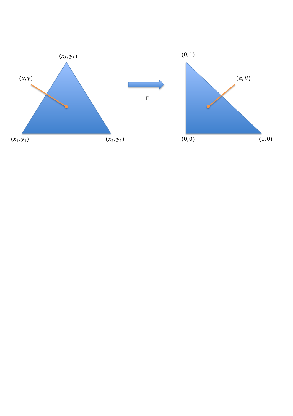
In Section 5 we discuss the implementation of the randomized quadrature formulas. Essentially, this is achieved by a transformation to a reference triangle, typically the 22-simplex, and a general rejection algorithm. Finally, we report on some numerical experiments in Section 6.

2. Notation and preliminaries

In this section, we fix some notation and introduce several function spaces, which are used throughout this paper. We also revisit the variational formulation of the boundary value problem (1) and its approximation by the finite element method. The section also contains a brief overview of some terminology from probability.

By ℕ{\mathbb{N}} we denote the set of all positive integers, while ℕ0:=ℕ∪{0}{\mathbb{N}}_{0}:={\mathbb{N}}\cup\{0\}. As usual, the set ℝ{\mathbb{R}} consists of all real numbers. By |⋅||\cdot| we denote the Euclidean norm on the Euclidean space ℝd{\mathbb{R}}^{d} for any d∈ℕd\in{\mathbb{N}}. In particular, if d=1d=1 then |⋅||\cdot| coincides with taking the absolute value.

Throughout this paper we often use CC as a generic constant, which may vary from appearance to appearance. However, CC is not allowed to depend on numerical parameters such as h∈(0,1]h\in(0,1].

Next, let us introduce some function spaces. Throughout this paper, we assume that 𝒟⊂ℝ2{\mathcal{D}}\subset{\mathbb{R}}^{2} is a bounded, convex and polygonal domain. By Lp​(𝒟)L^{p}({\mathcal{D}}), p∈[1,∞]p\in[1,\infty], we denote the Banach space of (equivalence classes of) pp-fold Lebesgue integrable functions, which is endowed with the norm

‖f‖Lp​(𝒟)\displaystyle\|f\|_{L^{p}({\mathcal{D}})} =(∫𝒟|f⁡(x)|p​𝑑x)1p for ​p∈[1,∞),\displaystyle=\Big(\int_{\mathcal{D}}|f(x)|^{p}\,\mathrm{d}x\Big)^{\frac{1}{p}}\quad\text{ for }p\in[1,\infty),
‖f‖L∞​(𝒟)\displaystyle\|f\|_{L^{\infty}({\mathcal{D}})} =ess​supx∈𝒟⁡|f⁡(x)|.\displaystyle=\esssup_{x\in{\mathcal{D}}}|f(x)|.

As it is customary, we do not distinguish notationally between functions and their equivalence classes.

An important example of an element in Lp​(𝒟)L^{p}({\mathcal{D}}) for any value of p∈[1,∞]p\in[1,\infty] is the indicator function of a measurable set B⊆𝒟B\subseteq{\mathcal{D}} denoted by 𝕀B\mathbb{I}_{B}. This function fulfills 𝕀B​(x)=1\mathbb{I}_{B}(x)=1 if x∈Bx\in B, else 𝕀B​(x)=0\mathbb{I}_{B}(x)=0.

Moreover, we denote by Wk,p​(𝒟)⊂Lp​(𝒟)W^{k,p}({\mathcal{D}})\subset L^{p}({\mathcal{D}}), p∈[1,∞]p\in[1,\infty], k∈ℕk\in{\mathbb{N}}, the Sobolev space with differentiation index kk. To be more precise, Wk,p​(𝒟)W^{k,p}({\mathcal{D}}) consists of all pp-fold integrable functions that are kk-times partially differentiable in the weak sense and whose derivatives are also pp-fold integrable. If Wk,p​(𝒟)W^{k,p}({\mathcal{D}}) is endowed with the norm

‖f‖Wk,p​(𝒟)\displaystyle\|f\|_{W^{k,p}({\mathcal{D}})} =(∑α∈ℕ02,|α|≤k∥∂αf∥Lp​(𝒟)p)1p for p∈[1,∞),\displaystyle=\Big(\sum_{\alpha\in{\mathbb{N}}_{0}^{2},|\alpha|\leq k}\|\partial^{\alpha}f\|_{L^{p}({\mathcal{D}})}^{p}\Big)^{\frac{1}{p}}\quad\text{ for }p\in[1,\infty),
‖f‖Wk,∞​(𝒟)\displaystyle\|f\|_{W^{k,\infty}({\mathcal{D}})} =∑α∈ℕ02,|α|≤k‖∂αf‖L∞​(𝒟),\displaystyle=\sum_{\alpha\in{\mathbb{N}}_{0}^{2},|\alpha|\leq k}\|\partial^{\alpha}f\|_{L^{\infty}({\mathcal{D}})},

then it is also a Banach space. Here we make use of the standard multi-index notation for partial derivatives, that is, for α∈ℕ02\alpha\in{\mathbb{N}}_{0}^{2} we define |α|=α1+α2|\alpha|=\alpha_{1}+\alpha_{2} and

∂αf:=∂|α|∂x1α1∂x2α2​f.\displaystyle\partial^{\alpha}f:=\frac{\partial^{|\alpha|}}{\partial_{x_{1}}^{\alpha_{1}}\partial_{x_{2}}^{\alpha_{2}}}f.

Further, if p=2p=2 then L2​(𝒟)L^{2}({\mathcal{D}}) and Hk​(𝒟):=Wk,2​(𝒟)H^{k}({\mathcal{D}}):=W^{k,2}({\mathcal{D}}) are Hilbert spaces. The inner products are denoted by (⋅,⋅)L2​(𝒟)(\cdot,\cdot)_{L^{2}({\mathcal{D}})} and (⋅,⋅)Hk​(𝒟)(\cdot,\cdot)_{H^{k}({\mathcal{D}})}, respectively.

In order to incorporate homogeneous Dirichlet boundary conditions, we also introduce the space H01​(𝒟)H^{1}_{0}({\mathcal{D}}), which is defined as the closure of the set of all infinitely often differentiable functions with compact support in 𝒟{\mathcal{D}} with respect to the norm in H1​(𝒟)H^{1}({\mathcal{D}}), that is

H01(𝒟):=Cc∞​(𝒟)¯∥⋅∥H1​(𝒟).\displaystyle H^{1}_{0}({\mathcal{D}}):=\overline{C_{c}^{\infty}({\mathcal{D}})}^{\|\cdot\|_{H^{1}({\mathcal{D}})}}.

It is well-known that the standard H1​(𝒟)H^{1}({\mathcal{D}})-norm and the semi-norm

|f|H1​(𝒟)=(∑i=12‖∂∂xi​f‖L2​(𝒟)2)12=(∫𝒟|∇f|2​𝑑x)12\displaystyle|f|_{H^{1}({\mathcal{D}})}=\Big(\sum_{i=1}^{2}\Big\|\frac{\partial}{\partial x_{i}}f\Big\|_{L^{2}({\mathcal{D}})}^{2}\Big)^{\frac{1}{2}}=\Big(\int_{\mathcal{D}}|\nabla f|^{2}\,\mathrm{d}x\Big)^{\frac{1}{2}}

are equivalent on H01​(𝒟)H^{1}_{0}({\mathcal{D}}). In particular, the space (H01(𝒟),|⋅|H1​(𝒟),(⋅,⋅)H01​(𝒟))(H^{1}_{0}({\mathcal{D}}),|\cdot|_{H^{1}({\mathcal{D}})},(\cdot,\cdot)_{H^{1}_{0}({\mathcal{D}})}) is a separable Hilbert space. For a detailed introduction to Sobolev spaces we refer the reader, for instance, to [11, Chapter 5].

For a domain 𝒟⊂ℝ2{\mathcal{D}}\subset{\mathbb{R}}^{2}, p∈[1,∞)p\in[1,\infty), and s∈(0,1)s\in(0,1) the Sobolev–Slobodeckij norm ∥⋅∥Ws,p​(𝒟)\|\cdot\|_{W^{s,p}({\mathcal{D}})} is given by

(6) ‖f‖Ws,p​(𝒟)=(‖f‖Lp​(𝒟)p+∫𝒟∫𝒟|f⁡(x1)−f⁡(x2)|p|x1−x2|2+s​p​d​x2​d​x1)1p.\displaystyle\|f\|_{W^{s,p}({\mathcal{D}})}=\Big(\|f\|^{p}_{L^{p}({\mathcal{D}})}+\int_{{\mathcal{D}}}\int_{{\mathcal{D}}}\frac{|f(x_{1})-f(x_{2})|^{p}}{|x_{1}-x_{2}|^{2+sp}}\,\mathrm{d}x_{2}\,\mathrm{d}x_{1}\Big)^{\frac{1}{p}}.

Then, the fractional order Sobolev space Ws,p​(𝒟)W^{s,p}({\mathcal{D}}) consists of all f∈Lp​(𝒟)f\in L^{p}({\mathcal{D}}) satisfying ‖f‖Ws,p​(𝒟)<∞\|f\|_{W^{s,p}({\mathcal{D}})}<\infty. By |⋅|Ws,p​(𝒟)|\cdot|_{W^{s,p}({\mathcal{D}})} we denote the corresponding semi-norm, which only consists of the double integral part in (6). Further details on these spaces are found in [9].

Next, we revisit the variational formulation of the boundary value problem (1). If σ∈L∞​(𝒟)\sigma\in L^{\infty}({\mathcal{D}}), σ⁡(x)≥σ0>0\sigma(x)\geq\sigma_{0}>0 for almost every x∈𝒟x\in{\mathcal{D}}, and f∈L2​(𝒟)f\in L^{2}({\mathcal{D}}), then it is well-known that the bilinear form a:H01​(𝒟)×H01​(𝒟)→ℝa\colon H^{1}_{0}({\mathcal{D}})\times H^{1}_{0}({\mathcal{D}})\to{\mathbb{R}} and the linear functional F:H01​(𝒟)→ℝF\colon H^{1}_{0}({\mathcal{D}})\to{\mathbb{R}} given by

(7) a⁡(u,v)\displaystyle a(u,v) :=∫𝒟σ(x)∇u(x)⋅∇v(x)dx,\displaystyle:=\int_{\mathcal{D}}\sigma(x)\nabla u(x)\cdot\nabla v(x)\,\mathrm{d}x,
(8) F⁡(v)\displaystyle F(v) :=∫𝒟f⁡(x)​v​(x)​𝑑x\displaystyle:=\int_{\mathcal{D}}f(x)v(x)\,\mathrm{d}x

for all u,v∈H01​(𝒟)u,v\in H^{1}_{0}({\mathcal{D}}) are well-defined. Moreover, aa is strongly positive and bounded, that is, it holds

(9) a⁡(v,v)\displaystyle a(v,v) ≥σ0​|v|H1​(𝒟)2,\displaystyle\geq\sigma_{0}|v|_{H^{1}({\mathcal{D}})}^{2},
(10) |a⁡(u,v)|\displaystyle|a(u,v)| ≤‖σ‖L∞​(𝒟)​|u|H1​(𝒟)|​v|H1​(𝒟)\displaystyle\leq\|\sigma\|_{L^{\infty}({\mathcal{D}})}|u|_{H^{1}({\mathcal{D}})}|v|_{H^{1}({\mathcal{D}})}

for all u,v∈H01​(𝒟)u,v\in H^{1}_{0}({\mathcal{D}}). Further, FF is a bounded linear functional.

Therefore, the lemma of Lax–Milgram, cf. [11, Chapter 6], is applicable and ensures the existence of a unique weak solution u∈H01​(𝒟)u\in H^{1}_{0}({\mathcal{D}}) satisfying

(11) a⁡(u,v)=F⁡(v)for all ​v∈H01​(𝒟).\displaystyle a(u,v)=F(v)\quad\text{for all }v\in H^{1}_{0}({\mathcal{D}}).

Observe that (11) coincides with (2).

For the error analysis in Section 3 and Section 4, it will be necessary to impose the following additional regularity condition on the exact solution.

Assumption 2.1.

The variational problem (11) has a uniquely determined strong solution, i.e., the unique weak solution uu to (11) is an element of H01​(𝒟)∩H2​(𝒟)H^{1}_{0}({\mathcal{D}})\cap H^{2}({\mathcal{D}}).

We refer, for instance, to [13, Theorem 3.2.1.2], which gives sufficient conditions for the existence of a strong solution. For example, if 𝒟{\mathcal{D}} is a convex, bounded and open subset of ℝ2{\mathbb{R}}^{2} and if σ∈L∞​(𝒟)\sigma\in L^{\infty}({\mathcal{D}}) has a globally Lipschitz continuous extension on 𝒟¯\overline{{\mathcal{D}}}, then Assumption 2.1 is satisfied for every f∈L2​(𝒟)f\in L^{2}({\mathcal{D}}).

Next, we briefly review the finite element method for problem (1). To this end, let (𝒯h)h∈(0,1](\mathcal{T}_{h})_{h\in(0,1]} be a family of admissible triangulations of 𝒟{\mathcal{D}}. More precisely, for every h∈(0,1]h\in(0,1] it holds that each triangle T∈𝒯hT\in\mathcal{T}_{h} is an open subset of 𝒟{\mathcal{D}} satisfying

⋃T∈𝒯hT¯\displaystyle\bigcup_{T\in\mathcal{T}_{h}}\overline{T} =𝒟¯ and T∩T′=∅,for all T,T′∈𝒯h,T≠T′.\displaystyle=\overline{{\mathcal{D}}}\quad\text{ and }T\cap T^{\prime}=\emptyset,\quad\text{for all }T,T^{\prime}\in\mathcal{T}_{h},T\neq T^{\prime}.

Further, it is assumed that no vertex of any triangle lies in the interior of an edge of any other triangle of the triangulation, cf. [4, Definition 3.3.11]. Typically, the parameter h∈(0,1]h\in(0,1] denotes the maximal edge length of all triangles in 𝒯h\mathcal{T}_{h}. Moreover, the area of a triangle TT is denoted by |T||T|.

As usual, we define the finite element space ShS_{h} associated to a triangulation 𝒯h\mathcal{T}_{h}, h∈(0,1]h\in(0,1], by

Sh={vh∈C(𝒟¯):vh=0 on ∂𝒟,vh|T∈Π1∀T∈𝒯h}.\displaystyle S_{h}=\{v_{h}\in C(\overline{{\mathcal{D}}})\,:\,v_{h}=0\,\text{ on }\partial{\mathcal{D}},\,v_{h}|_{T}\in\Pi_{1}\,\forall T\in\mathcal{T}_{h}\}.

Hereby, the set Π1\Pi_{1} consists of all polynomials up to degree 11. The finite element space ShS_{h} is finite dimensional and Nh=dim(Sh)N_{h}=\dim(S_{h}) is called the number of degrees of freedom. It coincides with the number of interior nodes (zi)i=1Nh(z_{i})_{i=1}^{N_{h}} of the triangulation. By (φj)j=1Nh⊂Sh(\varphi_{j})_{j=1}^{N_{h}}\subset S_{h} we denote the standard Lagrange basis of ShS_{h} determined by φj​(zi)=δi,j\varphi_{j}(z_{i})=\delta_{i,j} for all i,j=1,…,Nhi,j=1,\ldots,N_{h}. Further details on the construction of finite element spaces are found, e.g., in [4, Chapter 3] or [28, Chapter 5].

For the error analysis in Section 3 and Section 4 we have to impose the following additional condition on the family of triangulations.

Assumption 2.2.

We assume that (𝒯h)h∈(0,1](\mathcal{T}_{h})_{h\in(0,1]} is a family of admissible and quasi-uniform triangulations. In particular, the interior angles of each triangle in 𝒯h\mathcal{T}_{h} are bounded from below by a positive constant, independently of hh. In addition, there exists c∈(0,∞)c\in(0,\infty) such that for every h∈(0,1]h\in(0,1] and T∈𝒯hT\in\mathcal{T}_{h} it holds that |T|≥c​h2|T|\geq ch^{2}.

The assumption enables us to make use of a maximum norm estimate for functions from the finite element space ShS_{h}, which we cite from [37, Lemma 6.4]: If Assumption 2.2 is satisfied then there exists C∈(0,∞)C\in(0,\infty), independently of h∈(0,1]h\in(0,1], such that

(12) ‖vh‖L∞​(𝒟)≤C​ℓh12​|vh|H1​(𝒟)\displaystyle\|v_{h}\|_{L^{\infty}({\mathcal{D}})}\leq C\ell_{h}^{\frac{1}{2}}|v_{h}|_{H^{1}({\mathcal{D}})}

for every vh∈Shv_{h}\in S_{h}, where ℓh=max⁡(1,log⁡(1/h))\ell_{h}=\max(1,\log(1/h)).

Further, we recall that for a quasi-uniform family of triangulations the following inverse estimate is satisfied

(13) |vh|H1​(𝒟)≤C​h−1​‖vh‖L2​(𝒟)\displaystyle|v_{h}|_{H^{1}({\mathcal{D}})}\leq Ch^{-1}\|v_{h}\|_{L^{2}({\mathcal{D}})}

for every vh∈Shv_{h}\in S_{h}, where CC is independent of the triangulation 𝒯h\mathcal{T}_{h}. For a proof of (13) we refer to [4, Section 4.5].

Next, we introduce the Ritz projector Rh:H01​(𝒟)→ShR_{h}\colon{H}^{1}_{0}({\mathcal{D}})\to S_{h} as the orthogonal projector onto ShS_{h} with respect to the bilinear form aa. To be more precise, as a consequence of the lemma of Lax–Milgram, for each v∈H01​(𝒟)v\in{H}^{1}_{0}({\mathcal{D}}) there exists a unique element Rh​v∈ShR_{h}v\in S_{h} fulfilling

(14) a⁡(Rh​v,vh)=a⁡(v,vh) for all ​vh∈Sh.\displaystyle a(R_{h}v,v_{h})=a(v,v_{h})\quad\text{ for all }v_{h}\in S_{h}.

Note that Rh:H01​(𝒟)→ShR_{h}\colon H^{1}_{0}({\mathcal{D}})\to S_{h} is a bounded linear operator. In addition, there exists C∈(0,∞)C\in(0,\infty) such that for every h∈(0,1]h\in(0,1] and v∈H01​(𝒟)∩H2​(𝒟)v\in H^{1}_{0}({\mathcal{D}})\cap H^{2}({\mathcal{D}}) it holds

(15) |(Rh−I)​v|H1​(𝒟)\displaystyle|(R_{h}-I)v|_{H^{1}({\mathcal{D}})} ≤C​h​‖v‖H2​(𝒟),\displaystyle\leq Ch\|v\|_{H^{2}({\mathcal{D}})},
(16) ‖(Rh−I)​v‖L2​(𝒟)\displaystyle\|(R_{h}-I)v\|_{L^{2}({\mathcal{D}})} ≤C​h2​‖v‖H2​(𝒟).\displaystyle\leq Ch^{2}\|v\|_{H^{2}({\mathcal{D}})}.

A proof is found, for instance, in [28, Theorem 5.5].

For the introduction and the error analysis of Monte Carlo methods, we also require some fundamental concepts from probability and stochastic analysis. For a general introduction readers are referred to standard monographs on this topic, for instance [23, 24]. For the measure theoretical background see also [3, 7].

First, let us recall that a probability space (Ω,ℱ,ℙ)(\Omega,\mathcal{F},{\mathbb{P}}) consists of a measurable space (Ω,ℱ)(\Omega,\mathcal{F}) endowed with a finite measure ℙ{\mathbb{P}} satisfying ℙ⁡(Ω)=1{\mathbb{P}}(\Omega)=1. The value ℙ⁡(A)∈[0,1]{\mathbb{P}}(A)\in[0,1] is interpreted as the probability of the event A∈ℱA\in{\mathcal{F}}. A mapping X:Ω→ℝdX\colon\Omega\to{\mathbb{R}}^{d}, d∈ℕd\in{\mathbb{N}}, is called a random variable if XX is ℱ/ℬ⁡(ℝd){\mathcal{F}}/\mathcal{B}({\mathbb{R}}^{d})-measurable, where ℬ⁡(ℝd)\mathcal{B}({\mathbb{R}}^{d}) denotes the Borel-σ\sigma-algebra generated by the set of all open subsets of ℝd{\mathbb{R}}^{d}. More precisely, it holds true that

X−1​(B)={ω∈Ω:X⁡(ω)∈B}∈ℱ\displaystyle X^{-1}(B)=\big\{\omega\in\Omega\,:\,X(\omega)\in B\big\}\in\mathcal{F}

for all B∈ℬ⁡(ℝd)B\in\mathcal{B}({\mathbb{R}}^{d}). Every random variable induces a probability measure on its image space. In fact, the measure ℙX:ℬ⁡(ℝd)→[0,1]{\mathbb{P}}_{X}\colon\mathcal{B}({\mathbb{R}}^{d})\to[0,1] given by ℙX​(B)=ℙ⁡(X−1​(B)){\mathbb{P}}_{X}(B)={\mathbb{P}}(X^{-1}(B)) for all B∈ℬ⁡(ℝd)B\in\mathcal{B}({\mathbb{R}}^{d}) is a probability measure on the measurable space (ℝd,ℬ⁡(ℝd))({\mathbb{R}}^{d},\mathcal{B}({\mathbb{R}}^{d})). Usually, ℙX{\mathbb{P}}_{X} is called the distribution of XX.

If the distribution ℙX{\mathbb{P}}_{X} of XX is absolutely continuous with respect to the Lebesgue measure, then there exists a measurable, non-negative mapping gX:ℝd→ℝg_{X}\colon{\mathbb{R}}^{d}\to{\mathbb{R}} with

ℙX​(B)=ℙ⁡(X−1​(B))=∫BgX​(x)​𝑑x\displaystyle{\mathbb{P}}_{X}(B)={\mathbb{P}}(X^{-1}(B))=\int_{B}g_{X}(x)\,\mathrm{d}x

for every B∈ℬ⁡(ℝd)B\in\mathcal{B}({\mathbb{R}}^{d}). The mapping gXg_{X} is called the probability density function of XX and we write X∼gX​(x)​d​xX\sim g_{X}(x)\,\mathrm{d}x.

Next, let us recall that a random variable X:Ω→ℝdX\colon\Omega\to{\mathbb{R}}^{d} is called integrable if ∫Ω|X⁡(ω)|​𝑑ℙ​(ω)<∞\int_{\Omega}|X(\omega)|\,\mathrm{d}{\mathbb{P}}(\omega)<\infty. Then, the expectation of XX is defined as

𝔼⁡[X]:=∫ΩX⁡(ω)​𝑑ℙ​(ω)=∫ℝdx​d​ℙX​(x).{\mathbb{E}}[X]:=\int_{\Omega}X(\omega)\,\mathrm{d}{\mathbb{P}}(\omega)=\int_{{\mathbb{R}}^{d}}x\,\mathrm{d}{\mathbb{P}}_{X}(x).

We say that XX is centered if 𝔼⁡[X]=0{\mathbb{E}}[X]=0.

Moreover, we write X∈Lp​(Ω,ℝd)X\in L^{p}(\Omega;{\mathbb{R}}^{d}) with p∈[1,∞)p\in[1,\infty) if ∫Ω|X⁡(ω)|p​𝑑ℙ​(ω)<∞\int_{\Omega}|X(\omega)|^{p}\,\mathrm{d}{\mathbb{P}}(\omega)<\infty. If d=1d=1, then we simply write Lp​(Ω):=Lp​(Ω,ℝ)L^{p}(\Omega):=L^{p}(\Omega;{\mathbb{R}}). In addition, the set Lp​(Ω,ℝd)L^{p}(\Omega;{\mathbb{R}}^{d}) becomes a Banach space if we identify all random variables that only differ on a set of measure zero (i.e. probability zero) and if we endow Lp​(Ω,ℝd)L^{p}(\Omega;{\mathbb{R}}^{d}) with the norm

‖X‖Lp​(Ω,ℝd)=(𝔼⁡[|X|p])1p=(∫Ω|X⁡(ω)|p​𝑑ℙ​(ω))1p.\displaystyle\|X\|_{L^{p}(\Omega;{\mathbb{R}}^{d})}=\big({\mathbb{E}}\big[|X|^{p}\big]\big)^{\frac{1}{p}}=\Big(\int_{\Omega}|X(\omega)|^{p}\,\mathrm{d}{\mathbb{P}}(\omega)\Big)^{\frac{1}{p}}.

In Section 3, we frequently encounter a family of 𝒰⁡(T)\mathcal{U}(T)-distributed random variables (ZT)T∈𝒯h(Z_{T})_{T\in\mathcal{T}_{h}}. This means that for each T∈𝒯T\in\mathcal{T} the mapping ZT:Ω→ℝ2Z_{T}\colon\Omega\to{\mathbb{R}}^{2} is a random variable that is uniformly distributed on the triangle TT. More precisely, the distribution ℙZT{\mathbb{P}}_{Z_{T}} of ZTZ_{T} is given by ℙZT​(A)=|A∩T||T|{\mathbb{P}}_{Z_{T}}(A)=\frac{|A\cap T|}{|T|} for every A∈ℬ⁡(ℝ2)A\in{\mathcal{B}}({\mathbb{R}}^{2}). Moreover, it follows from the transformation theorem that the expectation of v∘ZTv\circ Z_{T} for an arbitrary function v∈L1​(𝒟)v\in L^{1}({\mathcal{D}}) is given by

𝔼⁡[v⁡(ZT)]=∫Tv⁡(z)​1|T|​𝑑z=∫𝒟v⁡(z)​1|T|​𝕀T​(z)​𝑑z,{\mathbb{E}}[v(Z_{T})]=\int_{T}v(z)\frac{1}{|T|}\,\mathrm{d}z=\int_{{\mathcal{D}}}v(z)\frac{1}{|T|}\mathbb{I}_{T}(z)\,\mathrm{d}z,

where the mapping gZT​(z)=1|T|​𝕀T​(z)g_{Z_{T}}(z)=\frac{1}{|T|}\mathbb{I}_{T}(z), z∈𝒟⊂ℝ2z\in{\mathcal{D}}\subset{\mathbb{R}}^{2}, is the probability density function of ZTZ_{T}.

Further, we say that a family of ℝd{\mathbb{R}}^{d}-valued random variables (Xn)n∈ℕ(X_{n})_{n\in{\mathbb{N}}} is independent if for any finite subset M⊂ℕM\subset{\mathbb{N}} and for arbitrary events (Am)m∈M⊂ℬ⁡(ℝd)(A_{m})_{m\in M}\subset\mathcal{B}({\mathbb{R}}^{d}) we have the multiplication rule

ℙ⁡(⋂m∈M{ω∈Ω:Xm​(ω)∈Am})=∏m∈Mℙ⁡({ω∈Ω:Xm​(ω)∈Am}).\displaystyle{\mathbb{P}}\Big(\bigcap_{m\in M}\{\omega\in\Omega\,:\,X_{m}(\omega)\in A_{m}\}\Big)=\prod_{m\in M}{\mathbb{P}}\big(\{\omega\in\Omega\,:\,X_{m}(\omega)\in A_{m}\}\big).

On the level of distributions this basically means that the joint distribution of each finite subfamily (Xm)m∈M(X_{m})_{m\in M} is equal to the product measure of the single distributions. This directly implies the multiplication rule for the expectation

(17) 𝔼⁡[∏m∈MXm]=∏m∈M𝔼⁡[Xm],\displaystyle{\mathbb{E}}\Big[\prod_{m\in M}X_{m}\Big]=\prod_{m\in M}{\mathbb{E}}\big[X_{m}\big],

provided XmX_{m} is integrable for each m∈Mm\in M.

Finally, let us mention that we often encounter random variables taking values in a function space instead of ℝd{\mathbb{R}}^{d}. For instance, in Theorem 3.3 we construct a random variable with values in Sh⊂H01​(𝒟)S_{h}\subset H^{1}_{0}({\mathcal{D}}). Since ShS_{h} is finite dimensional all notions for ℝd{\mathbb{R}}^{d}-valued random variables carry over to this case in a straight-forward way. However, we often use the norm of the Bochner space Lp​(Ω,V)L^{p}(\Omega;V) with either V=H01​(𝒟)V=H^{1}_{0}({\mathcal{D}}) or V=L2​(𝒟)V=L^{2}({\mathcal{D}}), which is given by

‖X‖Lp​(Ω,V)=(𝔼⁡[‖X‖Vp])1p=(∫Ω‖X⁡(ω)‖Vp​𝑑ℙ​(ω))1p\displaystyle\|X\|_{L^{p}(\Omega;V)}=\big({\mathbb{E}}\big[\|X\|^{p}_{V}\big]\big)^{\frac{1}{p}}=\Big(\int_{\Omega}\|X(\omega)\|^{p}_{V}\,\mathrm{d}{\mathbb{P}}(\omega)\Big)^{\frac{1}{p}}

for p∈[1,∞)p\in[1,\infty). For an introduction to Bochner spaces we refer to [7, Appendix E].

3. A randomized quadrature formula on a triangulation

As already mentioned in the introduction, quadrature rules are often used for the assembly of the matrix-vector system (4) associated to the finite element method for (11). In this section, we introduce a randomized quadrature formula, which is linked to the underlying triangulation 𝒯h\mathcal{T}_{h} of the finite element space ShS_{h}. We discuss the well-posedness of the resulting method and derive error estimates in a similar way as for deterministic quadrature rules shown in [28, Section 5.6].

Let 𝒯h\mathcal{T}_{h}, h∈(0,1]h\in(0,1], be an admissible triangulation of 𝒟{\mathcal{D}}. For a given v∈L1​(𝒟)v\in L^{1}({\mathcal{D}}), we consider the following Monte Carlo estimator

(18) QM​C​[v]:=∑T∈𝒯h|T|​v​(ZT),\displaystyle Q_{MC}[v]:=\sum_{T\in\mathcal{T}_{h}}|T|v(Z_{T}),

where we sum over all triangles of the triangulation 𝒯h\mathcal{T}_{h}. Hereby, (ZT)T∈𝒯h(Z_{T})_{T\in\mathcal{T}_{h}} denotes an independent family of random variables such that for each triangle T∈𝒯hT\in\mathcal{T}_{h} the random variable ZTZ_{T} is uniformly distributed on TT, that is ZT∼𝒰⁡(T)Z_{T}\sim\mathcal{U}(T). We discuss the simulation of ZTZ_{T} and the implementation of QM​CQ_{MC} in Subsection 5.4.

Observe that the randomized quadrature rule is independent of the considered equivalence class of v∈L1​(𝒟)v\in L^{1}({\mathcal{D}}). If v​(x)=v~​(x)v(x)=\tilde{v}(x) for almost every x∈𝒟x\in{\mathcal{D}}, then it follows that QM​C​[v]=QM​C​[v~]Q_{MC}[v]=Q_{MC}[\tilde{v}] with probability one.

Lemma 3.1.

Let 𝒯h\mathcal{T}_{h} be an admissible triangulation with maximal edge length h∈(0,1]h\in(0,1]. Then, the random quadrature rule QM​CQ_{MC} is unbiased, i.e., for every v∈L1​(𝒟)v\in L^{1}({\mathcal{D}}) it holds

𝔼⁡[QM​C​[v]]=∫𝒟v⁡(x)​𝑑x.\displaystyle{\mathbb{E}}\big[Q_{MC}[v]\big]=\int_{\mathcal{D}}v(x)\,\mathrm{d}x.

Moreover, if v∈L2​(𝒟)v\in L^{2}({\mathcal{D}}) then it holds that

𝔼⁡[|∫𝒟v⁡(x)​𝑑x−QM​C​[v]|2]≤32​h2​‖v‖L2​(𝒟)2.\displaystyle{\mathbb{E}}\Big[\Big|\int_{\mathcal{D}}v(x)\,\mathrm{d}x-Q_{MC}[v]\Big|^{2}\Big]\leq\frac{\sqrt{3}}{2}h^{2}\|v\|_{L^{2}({\mathcal{D}})}^{2}.

In addition, if v∈Ws,2​(𝒟)v\in W^{s,2}({\mathcal{D}}) for some s∈(0,1)s\in(0,1) then it follows that

𝔼⁡[|∫𝒟v⁡(x)​𝑑x−QM​C​[v]|2]≤h2+2​s​|v|Ws,2​(𝒟)2.\displaystyle{\mathbb{E}}\Big[\Big|\int_{\mathcal{D}}v(x)\,\mathrm{d}x-Q_{MC}[v]\Big|^{2}\Big]\leq h^{2+2s}|v|_{W^{s,2}({\mathcal{D}})}^{2}.
Proof.

Due to ZT∼1|T|​𝕀T​(z)​d​zZ_{T}\sim\frac{1}{|T|}\mathbb{I}_{T}(z)\,\mathrm{d}z for every T∈𝒯hT\in\mathcal{T}_{h} we have

𝔼⁡[|T|​v​(ZT)]=|T|∫𝒟v⁡(z)​1|T|​𝕀T​(z)​𝑑z=∫Tv⁡(z)​𝑑z.\displaystyle{\mathbb{E}}\big[|T|v(Z_{T})\big]=|T|\int_{\mathcal{D}}v(z)\frac{1}{|T|}\mathbb{I}_{T}(z)\,\mathrm{d}z=\int_{T}v(z)\,\mathrm{d}z.

Then the first assertion follows by summing over all triangles of the triangulation.

Now, let v∈L2​(𝒟)v\in L^{2}({\mathcal{D}}) be arbitrary. Then, the mean-square error is equal to

𝔼⁡[|∫𝒟v⁡(x)​𝑑x−QM​C​[v]|2]\displaystyle{\mathbb{E}}\Big[\Big|\int_{\mathcal{D}}v(x)\,\mathrm{d}x-Q_{MC}[v]\Big|^{2}\Big] =𝔼⁡[|∑T∈𝒯h(∫Tv⁡(x)​𝑑x−|T|​v​(ZT))|2]\displaystyle={\mathbb{E}}\Big[\Big|\sum_{T\in\mathcal{T}_{h}}\Big(\int_{T}v(x)\,\mathrm{d}x-|T|v(Z_{T})\Big)\Big|^{2}\Big]
=∑T∈𝒯h𝔼⁡[|∫Tv⁡(x)​𝑑x−|​T​|v⁡(ZT)|2]\displaystyle=\sum_{T\in\mathcal{T}_{h}}{\mathbb{E}}\Big[\Big|\int_{T}v(x)\,\mathrm{d}x-|T|v(Z_{T})\Big|^{2}\Big]

since the summands are independent and centered random variables. Therefore, they are orthogonal with respect to the L2​(Ω)L^{2}(\Omega)-inner product as can easily be deduced from (17).

Next, for every T∈𝒯hT\in\mathcal{T}_{h} we make use of ZT∼1|T|​𝕀T​(z)​d​zZ_{T}\sim\frac{1}{|T|}\mathbb{I}_{T}(z)\,\mathrm{d}z and the Cauchy–Schwarz inequality. This yields

𝔼⁡[|∫Tv⁡(x)​𝑑x−|​T​|v⁡(ZT)|2]\displaystyle{\mathbb{E}}\Big[\Big|\int_{T}v(x)\,\mathrm{d}x-|T|v(Z_{T})\Big|^{2}\Big] =|T|2​𝔼​[|1|T|​∫Tv⁡(x)​𝑑x−v⁡(ZT)|2]\displaystyle=|T|^{2}{\mathbb{E}}\Big[\Big|\frac{1}{|T|}\int_{T}v(x)\,\mathrm{d}x-v(Z_{T})\Big|^{2}\Big]
(19) =|T|​∫T|1|T|​∫Tv⁡(x)​𝑑x−v⁡(z)|2​𝑑z\displaystyle=|T|\int_{T}\Big|\frac{1}{|T|}\int_{T}v(x)\,\mathrm{d}x-v(z)\Big|^{2}\,\mathrm{d}z
≤∫T∫T|v⁡(x)−v⁡(z)|2​𝑑x​𝑑z.\displaystyle\leq\int_{T}\int_{T}\big|v(x)-v(z)\big|^{2}\,\mathrm{d}x\,\mathrm{d}z.

Then, since v∈L2​(𝒟)v\in L^{2}({\mathcal{D}}) we get

∫T∫T|v⁡(x)−v⁡(z)|2​𝑑x​𝑑z\displaystyle\int_{T}\int_{T}\big|v(x)-v(z)\big|^{2}\,\mathrm{d}x\,\mathrm{d}z =∫T∫T(v​(x)2−2​v​(x)​v​(z)+v​(z)2)​𝑑x​𝑑z\displaystyle=\int_{T}\int_{T}\big(v(x)^{2}-2v(x)v(z)+v(z)^{2}\big)\,\mathrm{d}x\,\mathrm{d}z
=2|T|∫T|v⁡(x)|2​𝑑x−2​(∫Tv⁡(x)​𝑑x)2\displaystyle=2|T|\int_{T}\big|v(x)\big|^{2}\,\mathrm{d}x-2\Big(\int_{T}v(x)\,\mathrm{d}x\Big)^{2}
≤2​|T|​∫T|v⁡(x)|2​𝑑x.\displaystyle\leq 2|T|\int_{T}\big|v(x)\big|^{2}\,\mathrm{d}x.

Then, we recall Weitzenböck’s inequality [38], which yields an upper bound for the area |T||T| of a triangle T∈𝒯hT\in\mathcal{T}_{h} with maximal edge length hh. More precisely, it holds

(20) |T|≤34​h2.\displaystyle|T|\leq\frac{\sqrt{3}}{4}h^{2}.

Hence, after summing over all triangles we obtain

‖∫𝒟v⁡(x)​𝑑x−QM​C​[v]‖L2​(Ω)2≤2​∑T∈𝒯h|T|​∫T|v⁡(x)|2​𝑑x≤32​h2​‖v‖L2​(𝒟)2.\displaystyle\Big\|\int_{\mathcal{D}}v(x)\,\mathrm{d}x-Q_{MC}[v]\Big\|_{L^{2}(\Omega)}^{2}\leq 2\sum_{T\in\mathcal{T}_{h}}|T|\int_{T}\big|v(x)\big|^{2}\,\mathrm{d}x\leq\frac{\sqrt{3}}{2}h^{2}\|v\|^{2}_{L^{2}({\mathcal{D}})}.

This proves the second claim.

Finally, let v∈Ws,2​(𝒟)v\in W^{s,2}({\mathcal{D}}), s∈(0,1)s\in(0,1). The estimate in (3) is then continued by

𝔼⁡[|∫Tv⁡(x)​𝑑x−|​T​|v⁡(ZT)|2]\displaystyle{\mathbb{E}}\Big[\Big|\int_{T}v(x)\,\mathrm{d}x-|T|v(Z_{T})\Big|^{2}\Big] ≤∫T∫T|v⁡(x)−v⁡(z)|2​𝑑x​𝑑z\displaystyle\leq\int_{T}\int_{T}\big|v(x)-v(z)\big|^{2}\,\mathrm{d}x\,\mathrm{d}z
≤h2+2​s​∫T∫T|v⁡(x)−v⁡(z)|2|x−z|2+2​s​𝑑x​𝑑z\displaystyle\leq h^{2+2s}\int_{T}\int_{T}\frac{\big|v(x)-v(z)\big|^{2}}{|x-z|^{2+2s}}\,\mathrm{d}x\,\mathrm{d}z
=h2+2​s​|v|Ws,2​(T)2\displaystyle=h^{2+2s}|v|_{W^{s,2}(T)}^{2}

since |x−z|≤h|x-z|\leq h for all x,y∈Tx,y\in T. After summing over all triangles we directly obtain the third assertion. ∎

Next, we apply the randomized quadrature formula (18) for the approximation of the bilinear form aa and the linear form FF defined in (7) and (8). From this we obtain two randomized mappings aM​C:Sh×Sh→L∞​(Ω)a_{MC}\colon S_{h}\times S_{h}\to L^{\infty}(\Omega) and FM​C:Sh→L2​(Ω)F_{MC}\colon S_{h}\to L^{2}(\Omega) which are given by

(21) aM​C(vh,wh):=QM​C[σ∇vh⋅∇wh]=∑T∈𝒯h|T|σ(ZT)∇vh(ZT)⋅∇wh(ZT)\displaystyle a_{MC}(v_{h},w_{h}):=Q_{MC}[\sigma\nabla v_{h}\cdot\nabla w_{h}]=\sum_{T\in\mathcal{T}_{h}}|T|\sigma(Z_{T})\nabla v_{h}(Z_{T})\cdot\nabla w_{h}(Z_{T})

and

(22) FM​C​(vh):=QM​C​[f​vh]=∑T∈𝒯h|T|​f​(ZT)​vh​(ZT)\displaystyle F_{MC}(v_{h}):=Q_{MC}[fv_{h}]=\sum_{T\in\mathcal{T}_{h}}|T|f(Z_{T})v_{h}(Z_{T})

for all vh,wh∈Shv_{h},w_{h}\in S_{h}. In passing, we observe that aM​C​(vh,wh)=a⁡(vh,wh)a_{MC}(v_{h},w_{h})=a(v_{h},w_{h}) if σ≡c∈(0,∞)\sigma\equiv c\in(0,\infty) in 𝒟{\mathcal{D}}. This holds true since the gradients of vh,wh∈Shv_{h},w_{h}\in S_{h} are constant on each triangle.

The next lemma answers the question of well-posedness of aM​Ca_{MC} and FM​CF_{MC} and contains some additional properties.

Lemma 3.2.

Let (𝒯h)h∈(0,1](\mathcal{T}_{h})_{h\in(0,1]} be a family of admissible triangulations of 𝒟{\mathcal{D}}. Assume that σ∈L∞​(𝒟)\sigma\in L^{\infty}({\mathcal{D}}) satisfies σ⁡(x)≥σ0>0\sigma(x)\geq\sigma_{0}>0 for almost every x∈𝒟x\in{\mathcal{D}}. Then, the mapping aM​Ca_{MC} introduced in (21) is well-defined for every h∈(0,1]h\in(0,1]. Moreover, it holds ℙ{\mathbb{P}}-almost surely that

|aM​C​(vh,wh)|\displaystyle|a_{MC}(v_{h},w_{h})| ≤‖σ‖L∞​(𝒟)​|vh|H1​(𝒟)|​wh|H1​(𝒟),\displaystyle\leq\|\sigma\|_{L^{\infty}({\mathcal{D}})}|v_{h}|_{H^{1}({\mathcal{D}})}|w_{h}|_{H^{1}({\mathcal{D}})},
aM​C​(vh,vh)\displaystyle a_{MC}(v_{h},v_{h}) ≥σ0​|vh|H1​(𝒟)2\displaystyle\geq\sigma_{0}|v_{h}|_{H^{1}({\mathcal{D}})}^{2}

for all vh,wh∈Shv_{h},w_{h}\in S_{h}.

In addition, if f∈L2​(𝒟)f\in L^{2}({\mathcal{D}}) and the family of triangulations satisfies Assumption 2.2 then the mapping FM​CF_{MC} defined in (22) is also well-defined and there exists C∈(0,∞)C\in(0,\infty) independent of 𝒯h\mathcal{T}_{h} with

|FM​C​(vh)|\displaystyle|F_{MC}(v_{h})| ≤C​ℓh12​QM​C​[|f|]|vh|H1​(𝒟)<∞ℙ-a.s.,\displaystyle\leq C\ell_{h}^{\frac{1}{2}}Q_{MC}[|f|]|v_{h}|_{H^{1}({\mathcal{D}})}<\infty\quad\text{${\mathbb{P}}$-a.s.},
‖FM​C​(vh)‖L2​(Ω)\displaystyle\|F_{MC}(v_{h})\|_{L^{2}(\Omega)} ≤C​‖f‖L2​(𝒟)​|vh|H1​(𝒟)\displaystyle\leq C\|f\|_{L^{2}({\mathcal{D}})}|v_{h}|_{H^{1}({\mathcal{D}})}

for all vh∈Shv_{h}\in S_{h}, where ℓh=max⁡(1,log⁡(1/h))\ell_{h}=\max(1,\log(1/h)).

Proof.

We first show that aM​C​(vh,wh)∈L∞​(Ω)a_{MC}(v_{h},w_{h})\in L^{\infty}(\Omega) for every vh,wh∈Shv_{h},w_{h}\in S_{h}. To see this, we recall that the functions in ShS_{h} are linear on each triangle TT in 𝒯h\mathcal{T}_{h}. This implies that the gradient ∇vh\nabla v_{h} is piecewise constant for every vh∈Shv_{h}\in S_{h}. Hence, the random variables ∇vh​(ZT)\nabla v_{h}(Z_{T}), T∈𝒯hT\in\mathcal{T}_{h}, are, in fact, constant with probability one. This implies that

|T|​|∇vh​(ZT)|2=∫T|∇vh​(x)|2​𝑑xℙ-almost surely.\displaystyle|T||\nabla v_{h}(Z_{T})|^{2}=\int_{T}|\nabla v_{h}(x)|^{2}\,\mathrm{d}x\quad\text{${\mathbb{P}}$-almost surely.}

Together with the assumption σ∈L∞​(𝒟)\sigma\in L^{\infty}({\mathcal{D}}) it therefore follows that the summands in (21) are essentially bounded random variables. More precisely, it holds ℙ{\mathbb{P}}-almost surely that

|aM​C​(vh,wh)|\displaystyle|a_{MC}(v_{h},w_{h})| ≤∑T∈𝒯h|T|​σ​(ZT)​|∇vh​(ZT)|​|∇wh​(ZT)|\displaystyle\leq\sum_{T\in\mathcal{T}_{h}}|T|\sigma(Z_{T})|\nabla v_{h}(Z_{T})||\nabla w_{h}(Z_{T})|
≤‖σ‖L∞​(𝒟)​∑T∈𝒯h|T|​|∇vh​(ZT)|​|∇wh​(ZT)|\displaystyle\leq\|\sigma\|_{L^{\infty}({\mathcal{D}})}\sum_{T\in\mathcal{T}_{h}}|T||\nabla v_{h}(Z_{T})||\nabla w_{h}(Z_{T})|
≤‖σ‖L∞​(𝒟)​(∑T∈𝒯h|T|​|∇vh​(ZT)|2)12​(∑T∈𝒯h|T|​|∇wh​(ZT)|2)12\displaystyle\leq\|\sigma\|_{L^{\infty}({\mathcal{D}})}\Big(\sum_{T\in\mathcal{T}_{h}}|T||\nabla v_{h}(Z_{T})|^{2}\Big)^{\frac{1}{2}}\Big(\sum_{T\in\mathcal{T}_{h}}|T||\nabla w_{h}(Z_{T})|^{2}\Big)^{\frac{1}{2}}
=‖σ‖L∞​(𝒟)​|vh|H1​(𝒟)|​wh|H1​(𝒟)\displaystyle=\|\sigma\|_{L^{\infty}({\mathcal{D}})}|v_{h}|_{H^{1}({\mathcal{D}})}|w_{h}|_{H^{1}({\mathcal{D}})}

for all vh,wh∈Shv_{h},w_{h}\in S_{h}.

Moreover, the same arguments yield for every vh∈Shv_{h}\in S_{h}

aM​C​(vh,vh)=∑T∈𝒯h|T|​σ​(ZT)​|∇vh​(ZT)|2≥σ0​|vh|H1​(𝒟)2ℙ-almost surely,\displaystyle a_{MC}(v_{h},v_{h})=\sum_{T\in\mathcal{T}_{h}}|T|\sigma(Z_{T})|\nabla v_{h}(Z_{T})|^{2}\geq\sigma_{0}|v_{h}|^{2}_{H^{1}({\mathcal{D}})}\quad\text{${\mathbb{P}}$-almost surely,}

since σ⁡(ZT)≥σ0>0\sigma(Z_{T})\geq\sigma_{0}>0 almost surely.

Next, we turn to the mapping FM​CF_{MC}. From (12) it follows for vh∈Shv_{h}\in S_{h} that

|FM​C​(vh)|\displaystyle|F_{MC}(v_{h})| ≤∑T∈𝒯h|T​‖f⁡(ZT)‖​vh​(ZT)|≤‖vh‖L∞​(𝒟)​QM​C​[|f|]\displaystyle\leq\sum_{T\in\mathcal{T}_{h}}|T||f(Z_{T})||v_{h}(Z_{T})|\leq\|v_{h}\|_{L^{\infty}({\mathcal{D}})}Q_{MC}[|f|]
≤C​ℓh12​QM​C​[|f|]​|vh|H1​(𝒟).\displaystyle\leq C\ell_{h}^{\frac{1}{2}}Q_{MC}[|f|]|v_{h}|_{H^{1}({\mathcal{D}})}.

Observe that the bound on the right-hand side still contains a random quadrature formula and is, therefore, itself random. However, for f∈L2​(𝒟)f\in L^{2}({\mathcal{D}}) it follows from applications of the Cauchy–Schwarz inequality and Lemma 3.1 that

𝔼⁡[(QM​C​[|f|])2]\displaystyle{\mathbb{E}}\big[(Q_{MC}[|f|])^{2}\big] =𝔼⁡[(∑T∈𝒯h|T|​|f⁡(ZT)|)2]\displaystyle={\mathbb{E}}\Big[\Big(\sum_{T\in\mathcal{T}_{h}}|T||f(Z_{T})|\Big)^{2}\Big]
≤|𝒟|​𝔼​[∑T∈𝒯h|T|​|f⁡(ZT)|2]\displaystyle\leq|{\mathcal{D}}|{\mathbb{E}}\Big[\sum_{T\in\mathcal{T}_{h}}|T||f(Z_{T})|^{2}\Big]
=|𝒟|​∫𝒟|f⁡(z)|2​𝑑z.\displaystyle=|{\mathcal{D}}|\int_{\mathcal{D}}|f(z)|^{2}\,\mathrm{d}z.

In particular, we have that QM​C​[|f|]<∞Q_{MC}[|f|]<\infty with probability one. This also proves that FM​C​(vh)∈L2​(Ω)F_{MC}(v_{h})\in L^{2}(\Omega). It remains to prove the asserted estimate of the L2​(Ω)L^{2}(\Omega)-norm of FM​C​(vh)F_{MC}(v_{h}). For this we first observe that

‖FM​C​(vh)‖L2​(Ω)2=‖FM​C​(vh)−𝔼⁡[FM​C​(vh)]‖L2​(Ω)2+(𝔼⁡[FM​C​(vh)])2\displaystyle\|F_{MC}(v_{h})\|^{2}_{L^{2}(\Omega)}=\big\|F_{MC}(v_{h})-{\mathbb{E}}[F_{MC}(v_{h})]\big\|^{2}_{L^{2}(\Omega)}+\big({\mathbb{E}}[F_{MC}(v_{h})]\big)^{2}

for every vh∈Shv_{h}\in S_{h}. From Lemma 3.1, the Cauchy–Schwarz inequality, and the Poincaré inequality on H01​(𝒟)H^{1}_{0}({\mathcal{D}}) it follows that

(𝔼⁡[FM​C​(vh)])2\displaystyle\big({\mathbb{E}}[F_{MC}(v_{h})]\big)^{2} =(∫𝒟f⁡(x)​vh​(x)​𝑑x)2\displaystyle=\Big(\int_{{\mathcal{D}}}f(x)v_{h}(x)\,\mathrm{d}x\Big)^{2}
≤∫𝒟|f⁡(x)|2​𝑑x​∫𝒟|vh​(x)|2​𝑑x≤C​‖f‖L2​(𝒟)2​|vh|H1​(𝒟)2,\displaystyle\leq\int_{{\mathcal{D}}}|f(x)|^{2}\,\mathrm{d}x\int_{{\mathcal{D}}}|v_{h}(x)|^{2}\,\mathrm{d}x\leq C\|f\|_{L^{2}({\mathcal{D}})}^{2}|v_{h}|_{H^{1}({\mathcal{D}})}^{2},

where the constant CC only depends on 𝒟{\mathcal{D}}. An application of Lemma 3.1 then yields

𝔼⁡[|FM​C​(vh)−𝔼⁡[FM​C​(vh)]|2]\displaystyle{\mathbb{E}}\big[\big|F_{MC}(v_{h})-{\mathbb{E}}[F_{MC}(v_{h})]\big|^{2}\big] =𝔼⁡[|QM​C​[f​vh]−∫𝒟f⁡(x)​vh​(x)​𝑑x|2]\displaystyle={\mathbb{E}}\Big[\Big|Q_{MC}[fv_{h}]-\int_{\mathcal{D}}f(x)v_{h}(x)\,\mathrm{d}x\Big|^{2}\Big]
≤32​h2​‖f​vh‖L2​(𝒟)2\displaystyle\leq\frac{\sqrt{3}}{2}h^{2}\|fv_{h}\|_{L^{2}({\mathcal{D}})}^{2}
≤32​h2​‖f‖L2​(𝒟)2​‖vh‖L∞​(𝒟)2\displaystyle\leq\frac{\sqrt{3}}{2}h^{2}\|f\|_{L^{2}({\mathcal{D}})}^{2}\|v_{h}\|_{L^{\infty}({\mathcal{D}})}^{2}
≤C​32​h2​ℓh​‖f‖L2​(𝒟)2​|vh|H1​(Ω)2,\displaystyle\leq C\frac{\sqrt{3}}{2}h^{2}\ell_{h}\|f\|_{L^{2}({\mathcal{D}})}^{2}|v_{h}|_{H^{1}(\Omega)}^{2},

where we also applied the maximum norm estimate (12). Hence, after taking note of suph∈(0,1]h2​ℓh=suph∈(0,1]h2​max⁡(1,log⁡(1/h))<∞\sup_{h\in(0,1]}h^{2}\ell_{h}=\sup_{h\in(0,1]}h^{2}\max(1,\log(1/h))<\infty the proof is completed. ∎

Next, we introduce the finite element problem based on the randomized quadrature rule. In terms of aM​Ca_{MC} and FM​CF_{MC} the problem is stated as follows:

(23) {Find uhM​C:Ω→Sh such that ℙ-almost surelyaM​C​(uhM​C,vh)=FM​C​(vh)​ for all ​vh∈Sh.\displaystyle\begin{cases}\text{Find }u_{h}^{MC}\colon\Omega\to S_{h}\text{ such that ${\mathbb{P}}$-almost surely}\\ a_{MC}(u_{h}^{MC},v_{h})=F_{MC}(v_{h})\text{ for all }v_{h}\in S_{h}.\end{cases}
Theorem 3.3.

Suppose that f∈L2​(𝒟)f\in L^{2}({\mathcal{D}}) and σ∈L∞​(𝒟)\sigma\in L^{\infty}({\mathcal{D}}) with σ⁡(x)≥σ0>0\sigma(x)\geq\sigma_{0}>0 for almost every x∈𝒟x\in{\mathcal{D}} are given. Then, for every admissible triangulation 𝒯h\mathcal{T}_{h}, h∈(0,1]h\in(0,1], there exists a uniquely determined solution uhM​C:Ω→Shu_{h}^{MC}\colon\Omega\to S_{h} to the discrete problem (23). In addition, there exists C∈(0,∞)C\in(0,\infty) independent of 𝒯h\mathcal{T}_{h} such that

|uhM​C|H1​(𝒟)\displaystyle|u_{h}^{MC}|_{H^{1}({\mathcal{D}})} ≤Cℓh12QM​C[|f|]ℙ-a.s.,\displaystyle\leq C\ell_{h}^{\frac{1}{2}}Q_{MC}[|f|]\quad\text{${\mathbb{P}}$-a.s.,}

where ℓh=max⁡(1,log⁡(1/h))\ell_{h}=\max(1,\log(1/h)).

Proof.

It follows from Lemma 3.2 that the bilinear form aM​Ca_{MC} is ℙ{\mathbb{P}}-almost surely strictly positive and bounded. Moreover, an inspection of the proof reveals that the exceptional set N1⊂ΩN_{1}\subset\Omega of probability zero, where these properties might be violated, can be chosen independently of the arguments vh,wh∈Shv_{h},w_{h}\in S_{h}. This is true since only the gradients of vhv_{h} and whw_{h} appear in aM​C​(vh,wh)a_{MC}(v_{h},w_{h}), which are piecewise constant on each triangle. Hence, on the set {ZT∈T}∈ℱ\{Z_{T}\in T\}\in{\mathcal{F}}, which has probability one, the randomness only occurs in the coefficient function σ\sigma. Therefore, for every ω∈Ω∖N1\omega\in\Omega\setminus N_{1} the mapping Sh×Sh∋(vh,wh)↦aM​C​(vh,wh)​(ω)∈ℝS_{h}\times S_{h}\ni(v_{h},w_{h})\mapsto a_{MC}(v_{h},w_{h})(\omega)\in{\mathbb{R}} satisfies the conditions of the lemma of Lax–Milgram.

In the same way, there exists a measurable set N2⊂ΩN_{2}\subset\Omega of probability zero such that the mapping Sh∋vh↦FM​C​(vh)​(ω)∈ℝS_{h}\ni v_{h}\mapsto F_{MC}(v_{h})(\omega)\in{\mathbb{R}} is a bounded linear functional on H01​(𝒟)H^{1}_{0}({\mathcal{D}}) for all ω∈Ω∖N2\omega\in\Omega\setminus N_{2}. In particular, we observe that the exceptional set N2N_{2} can again be chosen independently of the mapping vhv_{h} due to the continuity of all elements in ShS_{h}. In addition, the following estimate, which was used in the proof of Lemma 3.2, is true for all ω∈Ω\omega\in\Omega:

|vh​(ZT​(ω))|≤‖vh‖L∞​(𝒟).\displaystyle|v_{h}(Z_{T}(\omega))|\leq\|v_{h}\|_{L^{\infty}({\mathcal{D}})}.

Consequently, for every fixed ω∈Ω∖(N1∪N2)\omega\in\Omega\setminus(N_{1}\cup N_{2}) the lemma of Lax–Milgram uniquely determines an element uhM​C​(ω)∈Shu_{h}^{MC}(\omega)\in S_{h} satisfying

(24) aM​C​(uhM​C​(ω),vh)​(ω)=FM​C​(vh)​(ω)for all ​vh∈Sh.\displaystyle a_{MC}(u_{h}^{MC}(\omega),v_{h})(\omega)=F_{MC}(v_{h})(\omega)\quad\text{for all }v_{h}\in S_{h}.

Let us define uhM​C​(ω)=0∈Shu_{h}^{MC}(\omega)=0\in S_{h} for all ω∈N1∪N2\omega\in N_{1}\cup N_{2}. Next, we have to prove that the mapping Ω∋ω↦uhM​C​(ω)∈Sh\Omega\ni\omega\mapsto u_{h}^{MC}(\omega)\in S_{h} is measurable. However, this follows from an application of [10, Lemma 4.3] to the mapping g:Ω×ℝNh→ℝNhg\colon\Omega\times{\mathbb{R}}^{N_{h}}\to{\mathbb{R}}^{N_{h}} defined by g⁡(v,ω):=[aM​C​(∑i=1Nhvi​ψi,ψj)​(ω)−FM​C​(ψj)]j=1Nhg(v,\omega):=[a_{MC}(\sum_{i=1}^{N_{h}}v_{i}\psi_{i},\psi_{j})(\omega)-F_{MC}(\psi_{j})]_{j=1}^{N_{h}}, where v=[vi]i=1Nh∈ℝNhv=[v_{i}]_{i=1}^{N_{h}}\in{\mathbb{R}}^{N_{h}} and (ψj)j=1Nh⊂Sh(\psi_{j})_{j=1}^{N_{h}}\subset S_{h} is an arbitrary basis of the finite dimensional space ShS_{h}.

It remains to prove the stability estimate. Due to Lemma 3.2 and (24) it holds on Ω∖(N1∪N2)\Omega\setminus(N_{1}\cup N_{2}) that

σ0​|uhM​C|H1​(𝒟)2≤aM​C​(uhM​C,uhM​C)=FM​C​(uhM​C)≤C​ℓh12​QM​C​[|f|]​|uhM​C|H1​(𝒟).\displaystyle\sigma_{0}|u_{h}^{MC}|^{2}_{H^{1}({\mathcal{D}})}\leq a_{MC}(u_{h}^{MC},u_{h}^{MC})=F_{MC}(u_{h}^{MC})\leq C\ell_{h}^{\frac{1}{2}}Q_{MC}[|f|]|u_{h}^{MC}|_{H^{1}({\mathcal{D}})}.

Hence, after canceling the norm of uhM​Cu_{h}^{MC} one time on both sides of the inequality we obtain the desired estimate. ∎

Let us emphasize that the solution to the discrete problem (23) is a random variable. In fact, it follows directly from Theorem 3.3 that uhM​C∈Lp​(Ω,H01​(𝒟))u_{h}^{MC}\in L^{p}(\Omega;H^{1}_{0}({\mathcal{D}})) provided f∈Lp​(𝒟)f\in L^{p}({\mathcal{D}}) for p∈[2,∞]p\in[2,\infty].

As in the standard error analysis (cf. [28, Theorem 5.7]), we want to use uhM​Cu_{h}^{MC} as a test function in the discrete problem (23). However, in contrast to the situation in Lemma 3.1 we have, in general, that |𝔼⁡[FM​C​(vh)]−F⁡(𝔼⁡[vh])|≠0|{\mathbb{E}}[F_{MC}(v_{h})]-F({\mathbb{E}}[v_{h}])|\neq 0 for an arbitrary ShS_{h}-valued random function vh∈L2​(Ω,H01​(𝒟))v_{h}\in L^{2}(\Omega;H^{1}_{0}({\mathcal{D}})). The following lemma gives an estimate of this difference.

Lemma 3.4.

Let Assumption 2.2 be satisfied. Then, there exists C∈(0,∞)C\in(0,\infty) such that for every h∈(0,1]h\in(0,1], f∈Lp​(𝒟)f\in L^{p}({\mathcal{D}}), p∈[2,∞]p\in[2,\infty], and ShS_{h}-valued random variable vh∈L2​(Ω,H01​(𝒟))v_{h}\in L^{2}(\Omega;H^{1}_{0}({\mathcal{D}})) it holds

|𝔼⁡[FM​C​(vh)−F⁡(vh)]|≤{C​h1−2p​‖f‖Lp​(𝒟)​‖vh‖L2​(Ω,H01​(𝒟)), if ​p∈[2,∞),C​ℓh12​h​‖f‖L∞​(𝒟)​‖vh‖L2​(Ω,H01​(𝒟)), if ​p=∞,\displaystyle\big|{\mathbb{E}}\big[F_{MC}(v_{h})-F(v_{h})\big]\big|\leq\begin{cases}Ch^{1-\frac{2}{p}}\|f\|_{L^{p}({\mathcal{D}})}\|v_{h}\|_{L^{2}(\Omega;H^{1}_{0}({\mathcal{D}}))},&\quad\text{ if }p\in[2,\infty),\\ C\ell_{h}^{\frac{1}{2}}h\|f\|_{L^{\infty}({\mathcal{D}})}\|v_{h}\|_{L^{2}(\Omega;H^{1}_{0}({\mathcal{D}}))},&\quad\text{ if }p=\infty,\end{cases}

where ℓh=max⁡(1,log⁡(1/h))\ell_{h}=\max(1,\log(1/h)).

Proof.

For the error analysis it is convenient to choose an L2​(𝒟)L^{2}({\mathcal{D}})-orthonormal basis (ψj)j=1Nh(\psi_{j})_{j=1}^{N_{h}} of ShS_{h}, which solves the discrete eigenvalue problem

(25) a⁡(ψj,wh)=λh,j​(ψj,wh)L2​(𝒟)\displaystyle a(\psi_{j},w_{h})=\lambda_{h,j}(\psi_{j},w_{h})_{L^{2}({\mathcal{D}})}

for all wh∈Shw_{h}\in S_{h}. Hereby, 0<λh,1≤λh,2≤…≤λh,Nh0<\lambda_{h,1}\leq\lambda_{h,2}\leq\ldots\leq\lambda_{h,N_{h}} denote the discrete eigenvalues of the bilinear form aa on the finite element space Sh⊂H01​(𝒟)S_{h}\subset H^{1}_{0}({\mathcal{D}}). We refer to [28, Section 6.2] regarding the existence of (λh,j)j=1Nh(\lambda_{h,j})_{j=1}^{N_{h}} and the associated orthonormal basis (ψj)j=1Nh(\psi_{j})_{j=1}^{N_{h}}.

Next, let h∈(0,1]h\in(0,1], f∈Lp​(𝒟)f\in L^{p}({\mathcal{D}}), p∈[2,∞]p\in[2,\infty], and an ShS_{h}-valued random variable vh∈L2​(Ω,H01​(𝒟))v_{h}\in L^{2}(\Omega;H^{1}_{0}({\mathcal{D}})) be arbitrary. Then, we represent vhv_{h} in terms of the orthonormal basis (ψj)j=1Nh⊂Sh(\psi_{j})_{j=1}^{N_{h}}\subset S_{h} by

(26) vh=∑j=1Nhvj​ψj,\displaystyle v_{h}=\sum_{j=1}^{N_{h}}v_{j}\psi_{j},

For this choice of the basis, the random coefficients (vj)j=1Nh⊂L2​(Ω)(v_{j})_{j=1}^{N_{h}}\subset L^{2}(\Omega) are given by

vj=(vh,ψj)L2​(𝒟).\displaystyle v_{j}=(v_{h},\psi_{j})_{L^{2}({\mathcal{D}})}.

In particular, it follows from the Cauchy–Schwarz inequality that vjv_{j} is indeed a real-valued and square-integrable random variable for every j∈{1,…,Nh}j\in\{1,\ldots,N_{h}\}. Due to the linearity of FF and FM​CF_{MC} we then arrive at the estimate

|𝔼⁡[FM​C​(vh)−F⁡(vh)]|\displaystyle\big|{\mathbb{E}}\big[F_{MC}(v_{h})-F(v_{h})\big]\big| =|∑j=1Nh𝔼⁡[vj​(FM​C​(ψj)−F⁡(ψj))]|\displaystyle=\Big|\sum_{j=1}^{N_{h}}{\mathbb{E}}\big[v_{j}\big(F_{MC}(\psi_{j})-F(\psi_{j})\big)\big]\Big|
≤∑j=1Nh(𝔼⁡[|vj|2])12​(𝔼⁡[|FM​C​(ψj)−F⁡(ψj)|2])12\displaystyle\leq\sum_{j=1}^{N_{h}}\big({\mathbb{E}}\big[|v_{j}|^{2}\big]\big)^{\frac{1}{2}}\big({\mathbb{E}}\big[\big|F_{MC}(\psi_{j})-F(\psi_{j})\big|^{2}\big]\big)^{\frac{1}{2}}
≤(∑j=1Nhλh,j​𝔼​[|vj|2])12​(∑j=1Nhλh,j−1​𝔼​[|FM​C​(ψj)−F⁡(ψj)|2])12\displaystyle\leq\Big(\sum_{j=1}^{N_{h}}\lambda_{h,j}{\mathbb{E}}\big[|v_{j}|^{2}\big]\Big)^{\frac{1}{2}}\Big(\sum_{j=1}^{N_{h}}\lambda_{h,j}^{-1}{\mathbb{E}}\big[\big|F_{MC}(\psi_{j})-F(\psi_{j})\big|^{2}\big]\Big)^{\frac{1}{2}}

by additional applications of the Cauchy–Schwarz inequality. From (26) and (25) we then get

a⁡(vh,vh)=∑i,j=1Nhvj​vi​a​(ψj,ψi)=∑i,j=1Nhλh,j​vi​vj​(ψj,ψi)L2​(𝒟)=∑j=1Nhλh,j​vj2,\displaystyle a(v_{h},v_{h})=\sum_{i,j=1}^{N_{h}}v_{j}v_{i}a(\psi_{j},\psi_{i})=\sum_{i,j=1}^{N_{h}}\lambda_{h,j}v_{i}v_{j}(\psi_{j},\psi_{i})_{L^{2}({\mathcal{D}})}=\sum_{j=1}^{N_{h}}\lambda_{h,j}v_{j}^{2},

since (ψj)j=1Nh(\psi_{j})_{j=1}^{N_{h}} is an orthonormal basis of ShS_{h}. From this it follows that

(27) (∑j=1Nhλh,j​𝔼​[|vj|2])12=(𝔼⁡[a⁡(vh,vh)])12≤‖σ‖L∞​(𝒟)12​‖vh‖L2​(Ω,H01​(𝒟)).\displaystyle\Big(\sum_{j=1}^{N_{h}}\lambda_{h,j}{\mathbb{E}}\big[|v_{j}|^{2}\big]\Big)^{\frac{1}{2}}=\big({\mathbb{E}}\big[a(v_{h},v_{h})\big]\big)^{\frac{1}{2}}\leq\|\sigma\|_{L^{\infty}({\mathcal{D}})}^{\frac{1}{2}}\|v_{h}\|_{L^{2}(\Omega;H^{1}_{0}({\mathcal{D}}))}.

Moreover, an application of Lemma 3.1 yields

𝔼⁡[|FM​C​(ψj)−F⁡(ψj)|2]=𝔼⁡[|QM​C​(f​ψj)−∫𝒟f​ψj​𝑑x|2]≤32​h2​‖f​ψj‖L2​(𝒟)2\displaystyle{\mathbb{E}}\big[\big|F_{MC}(\psi_{j})-F(\psi_{j})\big|^{2}\big]={\mathbb{E}}\Big[\Big|Q_{MC}(f\psi_{j})-\int_{\mathcal{D}}f\psi_{j}\,\mathrm{d}x\Big|^{2}\Big]\leq\frac{\sqrt{3}}{2}h^{2}\|f\psi_{j}\|_{L^{2}({\mathcal{D}})}^{2}

for every j∈{1,…,Nh}j\in\{1,\ldots,N_{h}\}. Further, since f∈Lp​(𝒟)f\in L^{p}({\mathcal{D}}), p∈[2,∞]p\in[2,\infty], it follows from an application of Hölder’s inequality with conjugated exponent p′∈[2,∞]p^{\prime}\in[2,\infty] determined by 1p+1p′=12\frac{1}{p}+\frac{1}{p^{\prime}}=\frac{1}{2} that

‖f​ψj‖L2​(𝒟)≤‖f‖Lp​(𝒟)​‖ψj‖Lp′​(𝒟).\displaystyle\|f\psi_{j}\|_{L^{2}({\mathcal{D}})}\leq\|f\|_{L^{p}({\mathcal{D}})}\|\psi_{j}\|_{L^{p^{\prime}}({\mathcal{D}})}.

An application of the Gagliardo–Nierenberg inequality, cf. [33, Theorem 1.24], yields

‖ψj‖Lp′​(𝒟)≤C​‖ψj‖L2​(𝒟)2p′​|ψj|H1​(𝒟)1−2p′,\displaystyle\|\psi_{j}\|_{L^{p^{\prime}}({\mathcal{D}})}\leq C\|\psi_{j}\|_{L^{2}({\mathcal{D}})}^{\frac{2}{p^{\prime}}}|\psi_{j}|_{H^{1}({\mathcal{D}})}^{1-\frac{2}{p^{\prime}}},

where the constant CC is independent of j∈{1,…,Nh}j\in\{1,\ldots,N_{h}\}. Since ‖ψj‖L2​(𝒟)=1\|\psi_{j}\|_{L^{2}({\mathcal{D}})}=1 for every j∈{1,…,Nh}j\in\{1,\ldots,N_{h}\} and due to (9) and (25) we therefore obtain

‖ψj‖Lp′​(𝒟)≤C​|ψj|H1​(𝒟)2p≤Cσ01p​a​(ψj,ψj)1p≤Cσ01p​λh,j1p\displaystyle\|\psi_{j}\|_{L^{p^{\prime}}({\mathcal{D}})}\leq C|\psi_{j}|_{H^{1}({\mathcal{D}})}^{\frac{2}{p}}\leq\frac{C}{\sigma_{0}^{\frac{1}{p}}}a(\psi_{j},\psi_{j})^{\frac{1}{p}}\leq\frac{C}{\sigma_{0}^{\frac{1}{p}}}\lambda_{h,j}^{\frac{1}{p}}

for every p,p′∈[2,∞]p,p^{\prime}\in[2,\infty] with 1p+1p′=12\frac{1}{p}+\frac{1}{p^{\prime}}=\frac{1}{2}. Altogether, we have the bound

(28) ∑j=1Nhλh,j−1​𝔼​[|FM​C​(ψj)−F⁡(ψj)|2]≤32​h2​‖f‖Lp​(𝒟)2​∑j=1Nhλh,j−1​‖ψj‖Lp′​(𝒟)2≤C​h2​‖f‖Lp​(𝒟)2​∑j=1Nhλh,j−1+2p.\displaystyle\begin{split}\sum_{j=1}^{N_{h}}\lambda_{h,j}^{-1}{\mathbb{E}}\big[\big|F_{MC}(\psi_{j})-F(\psi_{j})\big|^{2}\big]&\leq\frac{\sqrt{3}}{2}h^{2}\|f\|_{L^{p}({\mathcal{D}})}^{2}\sum_{j=1}^{N_{h}}\lambda_{h,j}^{-1}\|\psi_{j}\|_{L^{p^{\prime}}({\mathcal{D}})}^{2}\\ &\leq Ch^{2}\|f\|_{L^{p}({\mathcal{D}})}^{2}\sum_{j=1}^{N_{h}}\lambda_{h,j}^{-1+\frac{2}{p}}.\end{split}

Concerning the last sum we recall from [28, Theorem 6.7] that

λj≤λh,j\displaystyle\lambda_{j}\leq\lambda_{h,j}

for all j∈{1,…,Nh}j\in\{1,\ldots,N_{h}\}, where (λj)j∈ℕ(\lambda_{j})_{j\in{\mathbb{N}}} denotes the family of eigenvalues of the bilinear form aa on the full space H01​(𝒟)H^{1}_{0}({\mathcal{D}}). Moreover, it is well-known, cf. [28, Section 6.1], that there exist constants c1,c2∈(0,∞)c_{1},c_{2}\in(0,\infty) only depending on σ\sigma and 𝒟{\mathcal{D}} such that

c1​j≤λj≤c2​j.\displaystyle c_{1}j\leq\lambda_{j}\leq c_{2}j.

From this it follows that

∑j=1Nhλh,j−1+2p\displaystyle\sum_{j=1}^{N_{h}}\lambda_{h,j}^{-1+\frac{2}{p}} ≤∑j=1Nhλj−1+2p≤c1−1+2p​∑j=1Nhj−1+2p≤c1−1+2p​(1+∫1Nhy−1+2p​𝑑y).\displaystyle\leq\sum_{j=1}^{N_{h}}\lambda_{j}^{-1+\frac{2}{p}}\leq c_{1}^{-1+\frac{2}{p}}\sum_{j=1}^{N_{h}}j^{-1+\frac{2}{p}}\leq c_{1}^{-1+\frac{2}{p}}\Big(1+\int_{1}^{N_{h}}y^{-1+\frac{2}{p}}\,\mathrm{d}y\Big).

Hence, we obtain

∑j=1Nhλh,j−1+2p≤{p2​c1−1+2p​Nh2p,if ​p∈[2,∞),c1−1​(1+log⁡(Nh)),if ​p=∞.\displaystyle\sum_{j=1}^{N_{h}}\lambda_{h,j}^{-1+\frac{2}{p}}\leq\begin{cases}\frac{p}{2}c_{1}^{-1+\frac{2}{p}}N_{h}^{\frac{2}{p}},&\quad\text{if }p\in[2,\infty),\\ c_{1}^{-1}(1+\log(N_{h})),&\quad\text{if }p=\infty.\end{cases}

From (25), (10), and the inverse estimate (13) it then follows that

Nh≤1c1​λh,Nh=1c1​a​(ψNh,ψNh)≤1c1​‖σ‖L∞​(𝒟)​|ψNh|H1​(𝒟)2≤C​h−2.\displaystyle N_{h}\leq\frac{1}{c_{1}}\lambda_{h,N_{h}}=\frac{1}{c_{1}}a(\psi_{N_{h}},\psi_{N_{h}})\leq\frac{1}{c_{1}}\|\sigma\|_{L^{\infty}({\mathcal{D}})}|\psi_{N_{h}}|^{2}_{H^{1}({\mathcal{D}})}\leq Ch^{-2}.

This implies that log⁡(Nh)≤C​max⁡(1,log⁡(1/h))=C​ℓh\log(N_{h})\leq C\max(1,\log(1/h))=C\ell_{h}. Altogether, this yields

(29) ∑j=1Nhλh,j−1+2p≤{C​h−4p,if ​p∈[2,∞),C​ℓh,if ​p=∞.\displaystyle\sum_{j=1}^{N_{h}}\lambda_{h,j}^{-1+\frac{2}{p}}\leq\begin{cases}Ch^{-\frac{4}{p}},&\quad\text{if }p\in[2,\infty),\\ C\ell_{h},&\quad\text{if }p=\infty.\end{cases}

Combining this with (27) and (28) then completes the proof. ∎

Next, we state and prove the main result of this section.

Theorem 3.5.

Suppose that σ∈L∞​(𝒟)∩Ws,q​(𝒟)\sigma\in L^{\infty}({\mathcal{D}})\cap W^{s,q}({\mathcal{D}}), s∈(0,1]s\in(0,1], q∈(2,∞)q\in(2,\infty), with σ⁡(x)≥σ0>0\sigma(x)\geq\sigma_{0}>0 for almost every x∈𝒟x\in{\mathcal{D}}. Let Assumptions 2.1 and 2.2 be satisfied. If f∈Lp​(𝒟)f\in L^{p}({\mathcal{D}}), p∈[2,∞)p\in[2,\infty), then it holds

‖u−uhM​C‖L2​(Ω,H01​(𝒟))\displaystyle\big\|u-u_{h}^{MC}\big\|_{L^{2}(\Omega;H^{1}_{0}({\mathcal{D}}))} ≤C​h​‖u‖H2​(𝒟)+C​hs​‖u‖H2​(𝒟)​|σ|Ws,q​(𝒟)+C​h1−2p​‖f‖Lp​(𝒟)\displaystyle\leq Ch\|u\|_{H^{2}({\mathcal{D}})}+Ch^{s}\|u\|_{H^{2}({\mathcal{D}})}|\sigma|_{W^{s,q}({\mathcal{D}})}+Ch^{1-\frac{2}{p}}\|f\|_{L^{p}({\mathcal{D}})}

for every h∈(0,1]h\in(0,1]. Further, if f∈L∞​(𝒟)f\in L^{\infty}({\mathcal{D}}) then it holds

‖u−uhM​C‖L2​(Ω,H01​(𝒟))\displaystyle\big\|u-u_{h}^{MC}\big\|_{L^{2}(\Omega;H^{1}_{0}({\mathcal{D}}))} ≤C​h​‖u‖H2​(𝒟)+C​hs​‖u‖H2​(𝒟)​|σ|Ws,q​(𝒟)+C​ℓh12​h​‖f‖L∞​(𝒟)\displaystyle\leq Ch\|u\|_{H^{2}({\mathcal{D}})}+Ch^{s}\|u\|_{H^{2}({\mathcal{D}})}|\sigma|_{W^{s,q}({\mathcal{D}})}+C\ell_{h}^{\frac{1}{2}}h\|f\|_{L^{\infty}({\mathcal{D}})}

for every h∈(0,1]h\in(0,1].

Proof.

Let us split the error into the following two parts

uhM​C−u=uhM​C−Rh​u+Rh​u−u=:θ+ρ,\displaystyle u_{h}^{MC}-u=u_{h}^{MC}-R_{h}u+R_{h}u-u=:\theta+\rho,

where Rh:H01​(𝒟)→ShR_{h}\colon H^{1}_{0}({\mathcal{D}})\to S_{h} denotes the Ritz projector (see Section 2). Observe that θ\theta and ρ\rho are orthogonal with respect to the bilinear form aa. Then, it follows from the positivity (9) and boundedness (10) of aa that

σ0​|uhM​C−u|H1​(𝒟)2\displaystyle\sigma_{0}|u_{h}^{MC}-u|^{2}_{H^{1}({\mathcal{D}})} ≤a⁡(uhM​C−u,uhM​C−u)=a⁡(θ,θ)+a⁡(ρ,ρ)\displaystyle\leq a(u_{h}^{MC}-u,u_{h}^{MC}-u)=a(\theta,\theta)+a(\rho,\rho)
≤‖σ‖L∞​(𝒟)​(|θ|H1​(𝒟)2+|​ρ|H1​(𝒟)2).\displaystyle\leq\|\sigma\|_{L^{\infty}({\mathcal{D}})}\big(|\theta|^{2}_{H^{1}({\mathcal{D}})}+|\rho|^{2}_{H^{1}({\mathcal{D}})}\big).

Standard error estimates for the conforming finite element method, cf. (15), yield

(30) |ρ|H1​(𝒟)=|Rh​u−u|H1​(𝒟)≤C​h​‖u‖H2​(𝒟).\displaystyle|\rho|_{H^{1}({\mathcal{D}})}=|R_{h}u-u|_{H^{1}({\mathcal{D}})}\leq Ch\|u\|_{H^{2}({\mathcal{D}})}.

Moreover, from (11) and (23) we get ℙ{\mathbb{P}}-almost surely for every vh∈Shv_{h}\in S_{h} that

aM​C​(θ,vh)\displaystyle a_{MC}(\theta,v_{h}) =aM​C​(uhM​C,vh)−aM​C​(Rh​u,vh)\displaystyle=a_{MC}(u_{h}^{MC},v_{h})-a_{MC}(R_{h}u,v_{h})
=FM​C​(vh)−F⁡(vh)+a⁡(Rh​u,vh)−aM​C​(Rh​u,vh),\displaystyle=F_{MC}(v_{h})-F(v_{h})+a(R_{h}u,v_{h})-a_{MC}(R_{h}u,v_{h}),

since F⁡(vh)=a⁡(u,vh)=a⁡(Rh​u,vh)F(v_{h})=a(u,v_{h})=a(R_{h}u,v_{h}) for every vh∈Shv_{h}\in S_{h}. In particular, for the choice vh=θ⁡(ω)=uhM​C​(ω)−Rh​u∈Shv_{h}=\theta(\omega)=u_{h}^{MC}(\omega)-R_{h}u\in S_{h} we obtain ℙ{\mathbb{P}}-almost surely that

σ0​|θ|H1​(𝒟)2≤aM​C​(θ,θ)=FM​C​(θ)−F⁡(θ)+a⁡(Rh​u,θ)−aM​C​(Rh​u,θ).\displaystyle\sigma_{0}|\theta|^{2}_{H^{1}({\mathcal{D}})}\leq a_{MC}(\theta,\theta)=F_{MC}(\theta)-F(\theta)+a(R_{h}u,\theta)-a_{MC}(R_{h}u,\theta).

From Lemma 3.2 and Theorem 3.3 it follows directly that all terms on the right-hand side are integrable with respect to ℙ{\mathbb{P}}. Hence, after taking expectations it remains to give error estimates for the two terms

E1\displaystyle E_{1} =|𝔼⁡[FM​C​(θ)−F⁡(θ)]|,\displaystyle=\big|{\mathbb{E}}\big[F_{MC}(\theta)-F(\theta)\big]\big|,
E2\displaystyle E_{2} =|𝔼⁡[a⁡(Rh​u,θ)−aM​C​(Rh​u,θ)]|.\displaystyle=\big|{\mathbb{E}}\big[a(R_{h}u,\theta)-a_{MC}(R_{h}u,\theta)\big]\big|.

An application of Lemma 3.4 directly yields

E1≤{C​h1−2p​‖f‖Lp​(𝒟)​‖θ‖L2​(Ω,H01​(𝒟)),if ​p∈[2,∞),C​ℓh12​h​‖f‖L∞​(𝒟)​‖θ‖L2​(Ω,H01​(𝒟)),if ​p=∞.\displaystyle E_{1}\leq\begin{cases}Ch^{1-\frac{2}{p}}\|f\|_{L^{p}({\mathcal{D}})}\|\theta\|_{L^{2}(\Omega;H^{1}_{0}({\mathcal{D}}))},&\quad\text{if }p\in[2,\infty),\\ C\ell_{h}^{\frac{1}{2}}h\|f\|_{L^{\infty}({\mathcal{D}})}\|\theta\|_{L^{2}(\Omega;H^{1}_{0}({\mathcal{D}}))},&\quad\text{if }p=\infty.\end{cases}

Next, we turn to the term E2E_{2} which is given by

E2\displaystyle E_{2} =|𝔼⁡[a⁡(Rh​u,θ)−aM​C​(Rh​u,θ)]|\displaystyle=\big|{\mathbb{E}}\big[a(R_{h}u,\theta)-a_{MC}(R_{h}u,\theta)\big]\big|
=|∑T∈𝒯h𝔼[∫Tσ(x)∇Rhu(x)⋅∇θ(x)dx−|T|σ(ZT)∇Rhu(ZT)⋅∇θ(ZT)]|.\displaystyle=\Big|\sum_{T\in\mathcal{T}_{h}}{\mathbb{E}}\Big[\int_{T}\sigma(x)\nabla R_{h}u(x)\cdot\nabla\theta(x)\,\mathrm{d}x-|T|\sigma(Z_{T})\nabla R_{h}u(Z_{T})\cdot\nabla\theta(Z_{T})\Big]\Big|.

Since Rh​u∈ShR_{h}u\in S_{h} and θ:Ω→Sh\theta\colon\Omega\to S_{h}, the respective gradients are constant on each triangle. Therefore, we have ∇Rhu(x)⋅∇θ(x)=∇Rhu(ZT)⋅∇θ(ZT)\nabla R_{h}u(x)\cdot\nabla\theta(x)=\nabla R_{h}u(Z_{T})\cdot\nabla\theta(Z_{T}) for every x∈Tx\in T. Hence, we get

E2\displaystyle E_{2} =|∑T∈𝒯h𝔼[(∫Tσ(x)dx−|T|σ(ZT))∇Rhu(ZT)⋅∇θ(ZT)]|\displaystyle=\Big|\sum_{T\in\mathcal{T}_{h}}{\mathbb{E}}\Big[\Big(\int_{T}\sigma(x)\,\mathrm{d}x-|T|\sigma(Z_{T})\Big)\nabla R_{h}u(Z_{T})\cdot\nabla\theta(Z_{T})\Big]\Big|
≤∑T∈𝒯h(𝔼[|(∫Tσ(x)dx−|T|σ(ZT))∇Rhu(ZT)|2])12(𝔼[|∇θ(ZT)|2])12\displaystyle\leq\sum_{T\in\mathcal{T}_{h}}\Big({\mathbb{E}}\Big[\Big|\Big(\int_{T}\sigma(x)\,\mathrm{d}x-|T|\sigma(Z_{T})\Big)\nabla R_{h}u(Z_{T})\Big|^{2}\Big]\Big)^{\frac{1}{2}}\big({\mathbb{E}}\big[|\nabla\theta(Z_{T})|^{2}\big]\big)^{\frac{1}{2}}
≤(∑T∈𝒯h|T|−1𝔼[(∫Tσ(x)dx−|T|σ(ZT))2|∇Rhu(ZT)|2])12\displaystyle\leq\Big(\sum_{T\in\mathcal{T}_{h}}|T|^{-1}{\mathbb{E}}\Big[\Big(\int_{T}\sigma(x)\,\mathrm{d}x-|T|\sigma(Z_{T})\Big)^{2}\big|\nabla R_{h}u(Z_{T})\big|^{2}\Big]\Big)^{\frac{1}{2}}
×(∑T∈𝒯h|T|​𝔼​[|∇θ​(ZT)|2])12\displaystyle\quad\times\Big(\sum_{T\in\mathcal{T}_{h}}|T|{\mathbb{E}}\big[|\nabla\theta(Z_{T})|^{2}\big]\Big)^{\frac{1}{2}}

by further applications of the Cauchy–Schwarz inequality. Moreover, by making again use of the fact that the gradient of θ\theta is piecewise constant we obtain

(∑T∈𝒯h|T|​𝔼​[|∇θ​(ZT)|2])12\displaystyle\Big(\sum_{T\in\mathcal{T}_{h}}|T|{\mathbb{E}}\big[|\nabla\theta(Z_{T})|^{2}\big]\Big)^{\frac{1}{2}} =(𝔼⁡[∑T∈𝒯h|T|​|∇θ​(ZT)|2])12\displaystyle=\Big({\mathbb{E}}\Big[\sum_{T\in\mathcal{T}_{h}}|T||\nabla\theta(Z_{T})|^{2}\Big]\Big)^{\frac{1}{2}}
=(𝔼⁡[∫𝒟|∇θ​(x)|2​𝑑x])12=‖θ‖L2​(Ω,H01​(𝒟)).\displaystyle=\Big({\mathbb{E}}\Big[\int_{\mathcal{D}}|\nabla\theta(x)|^{2}\,\mathrm{d}x\Big]\Big)^{\frac{1}{2}}=\|\theta\|_{L^{2}(\Omega;H^{1}_{0}({\mathcal{D}}))}.

Further, due to ZT∼|T|−1​𝕀T​(z)​d​zZ_{T}\sim|T|^{-1}\mathbb{I}_{T}(z)\,\mathrm{d}z it holds

(31) (∑T∈𝒯h|T|−1𝔼[(∫Tσ(x)dx−|T|σ(ZT))2|∇Rhu(ZT)|2])12=(∑T∈𝒯h|T|−2∫T(∫T(σ(x)−σ(z))dx)2|∇Rhu(z)|2dz)12≤(∑T∈𝒯h|T|−2∫T(∫T(σ(x)−σ(z))dx)2|∇(Rh−I)u(z)|2dz)12+(∑T∈𝒯h|T|−2​∫T(∫T(σ⁡(x)−σ⁡(z))​dx)2​|∇u​(z)|2​dz)12,\displaystyle\begin{split}&\Big(\sum_{T\in\mathcal{T}_{h}}|T|^{-1}{\mathbb{E}}\Big[\Big(\int_{T}\sigma(x)\,\mathrm{d}x-|T|\sigma(Z_{T})\Big)^{2}|\nabla R_{h}u(Z_{T})|^{2}\Big]\Big)^{\frac{1}{2}}\\ &\quad=\Big(\sum_{T\in\mathcal{T}_{h}}|T|^{-2}\int_{T}\Big(\int_{T}\big(\sigma(x)-\sigma(z)\big)\,\mathrm{d}x\Big)^{2}|\nabla R_{h}u(z)|^{2}\,\mathrm{d}z\Big)^{\frac{1}{2}}\\ &\quad\leq\Big(\sum_{T\in\mathcal{T}_{h}}|T|^{-2}\int_{T}\Big(\int_{T}\big(\sigma(x)-\sigma(z)\big)\,\mathrm{d}x\Big)^{2}|\nabla(R_{h}-I)u(z)|^{2}\,\mathrm{d}z\Big)^{\frac{1}{2}}\\ &\qquad+\Big(\sum_{T\in\mathcal{T}_{h}}|T|^{-2}\int_{T}\Big(\int_{T}\big(\sigma(x)-\sigma(z)\big)\,\mathrm{d}x\Big)^{2}|\nabla u(z)|^{2}\,\mathrm{d}z\Big)^{\frac{1}{2}},\end{split}

where we applied Minkowski’s inequality in the last step. The first term is then estimated by

(∑T∈𝒯h|T|−2∫T(∫T(σ(x)−σ(z))dx)2|∇(Rh−I)u(z)|2dz)12\displaystyle\Big(\sum_{T\in\mathcal{T}_{h}}|T|^{-2}\int_{T}\Big(\int_{T}\big(\sigma(x)-\sigma(z)\big)\,\mathrm{d}x\Big)^{2}|\nabla(R_{h}-I)u(z)|^{2}\,\mathrm{d}z\Big)^{\frac{1}{2}}
≤(∑T∈𝒯h|T|−1∫T∫T(σ(x)−σ(z))2dx|∇(Rh−I)u(z)|2dz)12\displaystyle\quad\leq\Big(\sum_{T\in\mathcal{T}_{h}}|T|^{-1}\int_{T}\int_{T}\big(\sigma(x)-\sigma(z)\big)^{2}\,\mathrm{d}x|\nabla(R_{h}-I)u(z)|^{2}\,\mathrm{d}z\Big)^{\frac{1}{2}}
≤C∥σ∥L∞​(𝒟)(∑T∈𝒯h∫T|∇(Rh−I)u(z)|2dz)12\displaystyle\quad\leq C\|\sigma\|_{L^{\infty}({\mathcal{D}})}\Big(\sum_{T\in\mathcal{T}_{h}}\int_{T}|\nabla(R_{h}-I)u(z)|^{2}\,\mathrm{d}z\Big)^{\frac{1}{2}}
≤C​‖σ‖L∞​(𝒟)​|(Rh−I)​u|H1​(𝒟)≤C​‖σ‖L∞​(𝒟)​‖u‖H2​(𝒟)​h\displaystyle\quad\leq C\|\sigma\|_{L^{\infty}({\mathcal{D}})}\big|(R_{h}-I)u\big|_{H^{1}({\mathcal{D}})}\leq C\|\sigma\|_{L^{\infty}({\mathcal{D}})}\|u\|_{H^{2}({\mathcal{D}})}h

by a further application of (30).

For the estimate of the last term in (31) we first consider s∈(0,1)s\in(0,1). Applying Hölder’s inequality with exponents ρ=q2∈(1,∞)\rho=\frac{q}{2}\in(1,\infty) and ρ′=qq−2∈(1,∞)\rho^{\prime}=\frac{q}{q-2}\in(1,\infty) yields

(∑T∈𝒯h|T|−2​∫T(∫T(σ⁡(x)−σ⁡(z))​𝑑x)2​|∇u​(z)|2​𝑑z)12\displaystyle\Big(\sum_{T\in\mathcal{T}_{h}}|T|^{-2}\int_{T}\Big(\int_{T}\big(\sigma(x)-\sigma(z)\big)\,\mathrm{d}x\Big)^{2}|\nabla u(z)|^{2}\,\mathrm{d}z\Big)^{\frac{1}{2}}
≤(∑T∈𝒯h|T|−2​(∫T(∫T|σ⁡(x)−σ⁡(z)|​𝑑x)2​ρ​𝑑z)1ρ​(∫T|∇u​(z)|2​ρ′​𝑑z)1ρ′)12\displaystyle\quad\leq\Big(\sum_{T\in\mathcal{T}_{h}}|T|^{-2}\Big(\int_{T}\Big(\int_{T}\big|\sigma(x)-\sigma(z)\big|\,\mathrm{d}x\Big)^{2\rho}\,\mathrm{d}z\Big)^{\frac{1}{\rho}}\Big(\int_{T}|\nabla u(z)|^{2\rho^{\prime}}\,\mathrm{d}z\Big)^{\frac{1}{\rho^{\prime}}}\Big)^{\frac{1}{2}}
≤(∑T∈𝒯h|T|−1ρ​(∫T∫T|σ⁡(x)−σ⁡(z)|2​ρ​𝑑x​𝑑z)1ρ​(∫T|∇u​(z)|2​ρ′​𝑑z)1ρ′)12\displaystyle\quad\leq\Big(\sum_{T\in\mathcal{T}_{h}}|T|^{-\frac{1}{\rho}}\Big(\int_{T}\int_{T}\big|\sigma(x)-\sigma(z)\big|^{2\rho}\,\mathrm{d}x\,\mathrm{d}z\Big)^{\frac{1}{\rho}}\Big(\int_{T}|\nabla u(z)|^{2\rho^{\prime}}\,\mathrm{d}z\Big)^{\frac{1}{\rho^{\prime}}}\Big)^{\frac{1}{2}}
≤(∑T∈𝒯h|T|−1​∫T∫T|σ⁡(x)−σ⁡(z)|q​𝑑x​𝑑z)1q​(∑T∈𝒯h∫T|∇u​(z)|2​ρ′​𝑑z)12​ρ′\displaystyle\quad\leq\Big(\sum_{T\in\mathcal{T}_{h}}|T|^{-1}\int_{T}\int_{T}\big|\sigma(x)-\sigma(z)\big|^{q}\,\mathrm{d}x\,\mathrm{d}z\Big)^{\frac{1}{q}}\Big(\sum_{T\in\mathcal{T}_{h}}\int_{T}|\nabla u(z)|^{2\rho^{\prime}}\,\mathrm{d}z\Big)^{\frac{1}{2\rho^{\prime}}}
≤(∑T∈𝒯h|T|−1​h2+q​s​∫T∫T|σ⁡(x)−σ⁡(z)|q|x−z|2+q​s​𝑑x​𝑑z)1q​‖u‖W1,2​ρ′​(𝒟)\displaystyle\quad\leq\Big(\sum_{T\in\mathcal{T}_{h}}|T|^{-1}h^{2+qs}\int_{T}\int_{T}\frac{\big|\sigma(x)-\sigma(z)\big|^{q}}{|x-z|^{2+qs}}\,\mathrm{d}x\,\mathrm{d}z\Big)^{\frac{1}{q}}\|u\|_{W^{1,2\rho^{\prime}}({\mathcal{D}})}

since |x−y|≤h|x-y|\leq h for all x,y∈Tx,y\in T.

Next, recall that the Sobolev embedding theorem [1, Theorem 4.12] yields

‖u‖W1,2​ρ′​(𝒟)≤C​‖u‖H2​(𝒟).\displaystyle\|u\|_{W^{1,2\rho^{\prime}}({\mathcal{D}})}\leq C\|u\|_{H^{2}({\mathcal{D}})}.

In addition, we have |T|−1≤c−1​h−2|T|^{-1}\leq c^{-1}h^{-2} due to Assumption 2.2. Altogether, this shows

(∑T∈𝒯h|T|−1​h2+q​s​∫T∫T|σ⁡(x)−σ⁡(z)|q|x−z|2+q​s​𝑑x​𝑑z)1q​‖u‖W1,2​ρ′​(𝒟)\displaystyle\Big(\sum_{T\in\mathcal{T}_{h}}|T|^{-1}h^{2+qs}\int_{T}\int_{T}\frac{\big|\sigma(x)-\sigma(z)\big|^{q}}{|x-z|^{2+qs}}\,\mathrm{d}x\,\mathrm{d}z\Big)^{\frac{1}{q}}\|u\|_{W^{1,2\rho^{\prime}}({\mathcal{D}})}
≤C​‖u‖H2​(𝒟)​|σ|Ws,q​(𝒟)​hs.\displaystyle\quad\leq C\|u\|_{H^{2}({\mathcal{D}})}|\sigma|_{W^{s,q}({\mathcal{D}})}h^{s}.

This completes the proof of the case s∈(0,1)s\in(0,1). The border case s=1s=1 follows by similar arguments and an additional application of the Poincaré–Wirtinger inequality. The details are left to the reader. ∎

4. Variance reduction by importance sampling

The goal of this section is to increase the accuracy of the randomized quadrature formula QM​CQ_{MC} introduced in (18) by applying a standard variance reduction technique for Monte Carlo methods termed importance sampling. An introduction to importance sampling and further variance reduction techniques is found, for instance, in [12, Chapter 6], [29, Chapter 3], and [31, Kapitel 5].

Let us briefly recall the main idea of importance sampling. Suppose one wants to approximate the integral

∫𝒟v⁡(x)​𝑑x,\displaystyle\int_{\mathcal{D}}v(x)\,\mathrm{d}x,

where v∈L2​(𝒟)v\in L^{2}({\mathcal{D}}) is given. Then, the standard Monte Carlo approach is to rewrite the integral as an expectation

𝔼⁡[v⁡(Z)]=|𝒟|∫𝒟−1⁡v⁡(x)​𝑑x,\displaystyle{\mathbb{E}}[v(Z)]=|{\mathcal{D}}|^{-1}\int_{{\mathcal{D}}}v(x)\,\mathrm{d}x,

where Z:Ω→𝒟Z\colon\Omega\to{\mathcal{D}} is a uniformly distributed random variable. In particular, the probability density function of ZZ is given by pZ​(x)=1|𝒟|​𝕀𝒟​(x)p_{Z}(x)=\frac{1}{|{\mathcal{D}}|}\mathbb{I}_{{\mathcal{D}}}(x). Then, the standard Monte Carlo estimator of the integral is defined as

|𝒟|M​∑i=1Mv⁡(Zi),\displaystyle\frac{|{\mathcal{D}}|}{M}\sum_{i=1}^{M}v(Z_{i}),

where (Zi)i=1M(Z_{i})_{i=1}^{M}, M∈ℕM\in{\mathbb{N}}, is a family of independent and identically distributed copies of ZZ. This estimator is unbiased and its variance is equal to

‖|𝒟|M​∑i=1Mv⁡(Zi)−∫𝒟v⁡(x)​𝑑x‖L2​(Ω)2\displaystyle\Big\|\frac{|{\mathcal{D}}|}{M}\sum_{i=1}^{M}v(Z_{i})-\int_{\mathcal{D}}v(x)\,\mathrm{d}x\Big\|_{L^{2}(\Omega)}^{2} =1M​var​(|𝒟|​v​(Z)).\displaystyle=\frac{1}{M}\mathrm{var}\big(|{\mathcal{D}}|v(Z)\big).

Therefore, the accuracy of the Monte Carlo estimator is determined by the number of samples M∈ℕM\in{\mathbb{N}} and the variance of the random variable |𝒟|​v​(Z)|{\mathcal{D}}|v(Z).

The main idea of importance sampling is then to increase the accuracy of the standard Monte Carlo estimator by replacing the uniformly distributed random variable ZZ with a random variable Y:Ω→𝒟Y\colon\Omega\to{\mathcal{D}} whose distribution is determined by a probability distribution function pYp_{Y}. If the density pYp_{Y} satisfies that pY​(x)=0p_{Y}(x)=0 only if v⁡(x)=0v(x)=0, then it follows from the transformation theorem that

∫𝒟v⁡(x)​𝑑x=∫𝒟v⁡(x)pY​(x)​pY​(x)​𝑑x=𝔼⁡[v⁡(Y)pY​(Y)].\displaystyle\int_{\mathcal{D}}v(x)\,\mathrm{d}x=\int_{\mathcal{D}}\frac{v(x)}{p_{Y}(x)}p_{Y}(x)\,\mathrm{d}x={\mathbb{E}}\Big[\frac{v(Y)}{p_{Y}(Y)}\Big].

From this one derives the following importance sampling estimator given by

1M​∑i=1Mv⁡(Yi)pY​(Yi),\displaystyle\frac{1}{M}\sum_{i=1}^{M}\frac{v(Y_{i})}{p_{Y}(Y_{i})},

where (Yi)i=1M(Y_{i})_{i=1}^{M} denotes a family of independent and identically distributed copies of YY. The art of importance sampling is then to determine a suitable density pYp_{Y} such that the variance is reduced and, at the same time, the generation of random variates with density pYp_{Y} is computational feasible and affordable. It is known (cf. [12, Theorem 6.5]) that the optimal choice of the density pYp_{Y} is

pY∗​(x)=|v⁡(x)|∫𝒟|v⁡(y)|​𝑑y, for ​x∈𝒟.\displaystyle p_{Y}^{\ast}(x)=\frac{|v(x)|}{\int_{\mathcal{D}}|v(y)|\,\mathrm{d}y},\quad\text{ for }x\in{\mathcal{D}}.

Observe that pY∗p_{Y}^{\ast} suggests to avoid sampling in regions of |𝒟||{\mathcal{D}}|, where |v||v| is zero or very small. However, since the denominator is typically unknown it is, in general, not possible to use the density pY∗p_{Y}^{\ast} in practice.

Nevertheless, one can often still make use of the underlying idea to improve the accuracy of the randomized quadrature rule (18). To demonstrate this, we solely focus on the Poisson equation

(32) {−Δ​u=f, in ​𝒟,u=0, on ​∂𝒟,\displaystyle\begin{cases}-\Delta u=f,&\quad\text{ in }{\mathcal{D}},\\ u=0,&\quad\text{ on }\partial{\mathcal{D}},\end{cases}

where 𝒟⊂ℝ2{\mathcal{D}}\subset{\mathbb{R}}^{2} is a convex, bounded and polygonal domain and f∈Lp​(𝒟)f\in L^{p}({\mathcal{D}}) for some p∈[2,∞]p\in[2,\infty].

Observe that the Poisson equation is a particular case of the boundary value problem (1) with σ≡1\sigma\equiv 1. In this case, the assembly of the stiffness matrix AhA_{h} in (4) does not require the application of a (randomized) quadrature rule.

Moreover, we recall that the entries of the load vector fh∈ℝNhf_{h}\in{\mathbb{R}}^{N_{h}} defined in (5) are given by

F⁡(φj)=∫𝒟f⁡(x)​φj​(x)​𝑑x,j∈{1,…,Nh},\displaystyle F(\varphi_{j})=\int_{{\mathcal{D}}}f(x)\varphi_{j}(x)\,\mathrm{d}x,\quad j\in\{1,\ldots,N_{h}\},

where (φj)j=1Nh(\varphi_{j})_{j=1}^{N_{h}} denotes the standard Lagrange basis of the finite element space ShS_{h}. According to the results in the previous section, these entries are then approximated by an application of the randomized quadrature formula (18) given by

FM​C​(φj)=QM​C​[f​φj]=∑T∈𝒯h|T|​f​(ZT)​φj​(ZT)\displaystyle F_{MC}(\varphi_{j})=Q_{MC}[f\varphi_{j}]=\sum_{T\in\mathcal{T}_{h}}|T|f(Z_{T})\varphi_{j}(Z_{T})

for every j∈{1,…,Nh}j\in\{1,\ldots,N_{h}\}. Observe that for each triangle T∈𝒯hT\in\mathcal{T}_{h} the term

(33) |T|​f​(ZT)​φj​(ZT)\displaystyle|T|f(Z_{T})\varphi_{j}(Z_{T})

can be regarded as a standard Monte Carlo estimator with only M=1M=1 sample for the integral

∫Tf⁡(x)​φj​(x)​𝑑x.\displaystyle\int_{T}f(x)\varphi_{j}(x)\,\mathrm{d}x.

The idea of this section is to replace this term by a suitable importance sampling estimator.

Since we do not want to impose any additional assumption on ff it is, as already mentioned above, not feasible to use the corresponding optimal density function pY∗p_{Y}^{\ast} with v=f​φjv=f\varphi_{j}. Instead, we recall that the piecewise linear basis function φj\varphi_{j} is equal to zero in two of the three vertices and equal to one in the remaining vertex of every triangle T∈𝒯hT\in\mathcal{T}_{h} with T∩supp⁡(φj)≠∅T\cap\mathrm{supp}(\varphi_{j})\neq\emptyset. In particular, this implies φj​(x)≥0\varphi_{j}(x)\geq 0 for every x∈Tx\in T. Further, it holds

∫Tφj​(x)​𝑑x=13​|T|.\displaystyle\int_{T}\varphi_{j}(x)\,\mathrm{d}x=\frac{1}{3}|T|.

Therefore, the mapping pT,j:𝒟→[0,∞)p_{T,j}\colon{\mathcal{D}}\to[0,\infty) defined by

(34) pT,j​(x)=3​|T|−1​φj​(x)​𝕀T​(x),x∈𝒟,\displaystyle p_{T,j}(x)=3|T|^{-1}\varphi_{j}(x)\mathbb{I}_{T}(x),\quad x\in{\mathcal{D}},

is a probability density function. By replacing ZTZ_{T} in (33) with a random variable YT,j∼pT,j​(x)​d​xY_{T,j}\sim p_{T,j}(x)\,\mathrm{d}x we arrive at the corresponding importance sampling estimator (again with only M=1M=1 sample)

f⁡(YT,j)​φj​(YT,j)pT,j​(YT,j)=13​|T|​f​(YT,j)\displaystyle\frac{f(Y_{T,j})\varphi_{j}(Y_{T,j})}{p_{T,j}(Y_{T,j})}=\frac{1}{3}|T|f(Y_{T,j})

for the integral ∫Tf⁡(x)​φj​(x)​𝑑x\int_{T}f(x)\varphi_{j}(x)\,\mathrm{d}x. Observe that the use of YT,jY_{T,j} significantly decreases the probability of the integrand f​φjf\varphi_{j} being evaluated at a point x∈Tx\in T close to a vertex, where the basis function φj\varphi_{j} is equal to zero. We discuss the simulation of the random variable YT,jY_{T,j} in Section 5.

To sum up, this suggests to use the linear mapping FI​S:Sh→L2​(Ω)F_{IS}\colon S_{h}\to L^{2}(\Omega) given by

(35) FI​S​(vh)=13​∑T∈𝒯h|T|​∑j=1T∩supp⁡(φj)≠∅Nhvj​f​(YT,j)\displaystyle F_{IS}(v_{h})=\frac{1}{3}\sum_{T\in\mathcal{T}_{h}}|T|\sum_{\begin{subarray}{c}j=1\\ T\cap\mathrm{supp}(\varphi_{j})\neq\emptyset\end{subarray}}^{N_{h}}v_{j}f(Y_{T,j})

for every vh=∑j=1Nhvj​φj∈Shv_{h}=\sum_{j=1}^{N_{h}}v_{j}\varphi_{j}\in S_{h}. Hereby, (YT,j)T∈𝒯h,j∈{1,…,Nh}(Y_{T,j})_{T\in\mathcal{T}_{h},j\in\{1,\ldots,N_{h}\}} is a family of independent random variables with YT,j∼pT,j​(x)​d​xY_{T,j}\sim p_{T,j}(x)\,\mathrm{d}x. In particular, the entries of the load vector fhf_{h} are then approximated by

FI​S​(φj)=13​∑T∈𝒯hT∩supp⁡(φj)≠∅|T|​f​(YT,j)\displaystyle F_{IS}(\varphi_{j})=\frac{1}{3}\sum_{\begin{subarray}{c}T\in\mathcal{T}_{h}\\ T\cap\mathrm{supp}(\varphi_{j})\neq\emptyset\end{subarray}}|T|f(Y_{T,j})

for every j∈{1,…,Nh}j\in\{1,\ldots,N_{h}\}. As the following lemma shows, the importance sampling estimator (35) is unbiased and convergent in the limit h→0h\to 0.

Lemma 4.1.

Let 𝒯h\mathcal{T}_{h} be an admissible triangulation with maximal edge length h∈(0,1]h\in(0,1]. Then, for every f∈L1​(𝒟)f\in L^{1}({\mathcal{D}}) and vh∈Shv_{h}\in S_{h} it holds that

𝔼⁡[FI​S​(vh)]=∫𝒟f⁡(x)​vh​(x)​𝑑x.\displaystyle{\mathbb{E}}\big[F_{IS}(v_{h})\big]=\int_{\mathcal{D}}f(x)v_{h}(x)\,\mathrm{d}x.

Further, if f∈Lp​(𝒟)f\in L^{p}({\mathcal{D}}), p∈[2,∞]p\in[2,\infty], then it holds for every vh∈Shv_{h}\in S_{h} that

‖∫𝒟f⁡(x)​vh​(x)​𝑑x−FI​S​(vh)‖L2​(Ω)\displaystyle\Big\|\int_{\mathcal{D}}f(x)v_{h}(x)\,\mathrm{d}x-F_{IS}(v_{h})\Big\|_{L^{2}(\Omega)}
≤1124​h​‖vh‖L∞​(𝒟)2p​‖f‖Lp​(𝒟)​(2​h​|vh|H1​(𝒟)+‖vh‖L2​(𝒟))1−2p.\displaystyle\quad\leq\frac{1}{\sqrt[4]{12}}h\|v_{h}\|_{L^{\infty}({\mathcal{D}})}^{\frac{2}{p}}\|f\|_{L^{p}({\mathcal{D}})}\big(2h|v_{h}|_{H^{1}({\mathcal{D}})}+\|v_{h}\|_{L^{2}({\mathcal{D}})}\big)^{1-\frac{2}{p}}.

In addition, if f∈Ws,2​(𝒟)f\in W^{s,2}({\mathcal{D}}) for some s∈(0,1)s\in(0,1) then it holds for every vh∈Shv_{h}\in S_{h} that

‖∫𝒟f⁡(x)​vh​(x)​𝑑x−FI​S​(vh)‖L2​(Ω)≤h1+s​‖vh‖L∞​(𝒟)​|f|Ws,2​(𝒟).\displaystyle\Big\|\int_{\mathcal{D}}f(x)v_{h}(x)\,\mathrm{d}x-F_{IS}(v_{h})\Big\|_{L^{2}(\Omega)}\leq h^{1+s}\|v_{h}\|_{L^{\infty}({\mathcal{D}})}|f|_{W^{s,2}({\mathcal{D}})}.
Proof.

Let vh=∑j=1Nhvj​φj∈Shv_{h}=\sum_{j=1}^{N_{h}}v_{j}\varphi_{j}\in S_{h} be arbitrary with coefficients (vj)j=1Nh⊂ℝ(v_{j})_{j=1}^{N_{h}}\subset{\mathbb{R}}. Due to YT,j∼3|T|​φj​(z)​𝕀T​(z)​d​zY_{T,j}\sim\frac{3}{|T|}\varphi_{j}(z)\mathbb{I}_{T}(z)\,\mathrm{d}z for every T∈𝒯hT\in\mathcal{T}_{h} we have

∑j=1Nhvj​𝔼​[|T|3​f​(YT,j)]=∑j=1Nhvj​|T|3​∫Tf⁡(z)​φj​(z)​3|T|​𝑑z=∫Tf⁡(z)​vh​(z)​𝑑z.\displaystyle\sum_{j=1}^{N_{h}}v_{j}{\mathbb{E}}\Big[\frac{|T|}{3}f(Y_{T,j})\Big]=\sum_{j=1}^{N_{h}}v_{j}\frac{|T|}{3}\int_{T}f(z)\varphi_{j}(z)\frac{3}{|T|}\,\mathrm{d}z=\int_{T}f(z)v_{h}(z)\,\mathrm{d}z.

Then, the first assertion follows by summing over all triangles of the triangulation.

Now, let f∈L2​(𝒟)f\in L^{2}({\mathcal{D}}) be arbitrary. In the same way as in the proof of Lemma 3.1, the mean-square error is shown to be equal to

‖∫𝒟f⁡(x)​vh​(x)​𝑑x−FI​S​(vh)‖L2​(Ω)2\displaystyle\Big\|\int_{\mathcal{D}}f(x)v_{h}(x)\,\mathrm{d}x-F_{IS}(v_{h})\Big\|_{L^{2}(\Omega)}^{2}
=∑T∈𝒯h∑j=1T∩supp⁡(φj)≠∅Nhvj2​𝔼​[|∫Tf⁡(x)​φj​(x)​𝑑x−|T|3​f​(YT,j)|2],\displaystyle\quad=\sum_{T\in\mathcal{T}_{h}}\sum_{\begin{subarray}{c}j=1\\ T\cap\mathrm{supp}(\varphi_{j})\neq\emptyset\end{subarray}}^{N_{h}}v_{j}^{2}{\mathbb{E}}\Big[\Big|\int_{T}f(x)\varphi_{j}(x)\,\mathrm{d}x-\frac{|T|}{3}f(Y_{T,j})\Big|^{2}\Big],

due to the independence of the random variables (YT,j)T∈𝒯h,j∈{1,…,Nh}(Y_{T,j})_{T\in\mathcal{T}_{h},j\in\{1,\ldots,N_{h}\}}.

Then, for every j∈{1,…,Nh}j\in\{1,\ldots,N_{h}\} and T∈𝒯hT\in\mathcal{T}_{h} with T∩supp⁡(φj)≠∅T\cap\mathrm{supp}(\varphi_{j})\neq\emptyset we make use of YT,j∼3|T|​𝕀T​(z)​φj​(z)​d​zY_{T,j}\sim\frac{3}{|T|}\mathbb{I}_{T}(z)\varphi_{j}(z)\,\mathrm{d}z and the Cauchy–Schwarz inequality. This yields

𝔼⁡[|∫Tf⁡(x)​φj​(x)​𝑑x−|T|3​f​(YT,j)|2]\displaystyle{\mathbb{E}}\Big[\Big|\int_{T}f(x)\varphi_{j}(x)\,\mathrm{d}x-\frac{|T|}{3}f(Y_{T,j})\Big|^{2}\Big]
=3|T|​∫T|∫Tf⁡(x)​φj​(x)​𝑑x−|T|3​f​(z)|2​φj​(z)​𝑑z\displaystyle\quad=\frac{3}{|T|}\int_{T}\Big|\int_{T}f(x)\varphi_{j}(x)\,\mathrm{d}x-\frac{|T|}{3}f(z)\Big|^{2}\varphi_{j}(z)\,\mathrm{d}z
=3|T|​∫T|∫T(f⁡(x)−f⁡(z))​φj​(x)​𝑑x|2​φj​(z)​𝑑z\displaystyle\quad=\frac{3}{|T|}\int_{T}\Big|\int_{T}(f(x)-f(z))\varphi_{j}(x)\,\mathrm{d}x\Big|^{2}\varphi_{j}(z)\,\mathrm{d}z
≤∫T∫T(f⁡(x)−f⁡(z))2​φj​(x)​φj​(z)​𝑑x​𝑑z\displaystyle\quad\leq\int_{T}\int_{T}(f(x)-f(z))^{2}\varphi_{j}(x)\varphi_{j}(z)\,\mathrm{d}x\,\mathrm{d}z
=23|T|∫T|f⁡(x)|2​φj​(x)​𝑑x−2​(∫Tf⁡(x)​φj​(x)​𝑑x)2.\displaystyle\quad=\frac{2}{3}|T|\int_{T}|f(x)|^{2}\varphi_{j}(x)\,\mathrm{d}x-2\Big(\int_{T}f(x)\varphi_{j}(x)\,\mathrm{d}x\Big)^{2}.

We neglect the last term and insert this estimate into the mean-square error. An application of Weitzenböck’s inequality (20) then yields

(36) ‖∫𝒟f⁡(x)​vh​(x)​dx−FI​S​(vh)‖L2​(Ω)2=∑T∈𝒯h∑j=1T∩supp⁡(φj)≠∅Nhvj2​𝔼​[|∫Tf⁡(x)​φj​(x)​𝑑x−|T|3​f​(YT,j)|2]≤23​∑T∈𝒯h∑j=1T∩supp⁡(φj)≠∅Nhvj2​|T|​∫T|f⁡(x)|2​φj​(x)​𝑑x≤12​3​h2​∑T∈𝒯h∑j=1T∩supp⁡(φj)≠∅Nhvj2​∫T|f⁡(x)|2​φj​(x)​dx.\displaystyle\begin{split}&\Big\|\int_{\mathcal{D}}f(x)v_{h}(x)\,\mathrm{d}x-F_{IS}(v_{h})\Big\|_{L^{2}(\Omega)}^{2}\\ &\quad=\sum_{T\in\mathcal{T}_{h}}\sum_{\begin{subarray}{c}j=1\\ T\cap\mathrm{supp}(\varphi_{j})\neq\emptyset\end{subarray}}^{N_{h}}v_{j}^{2}{\mathbb{E}}\Big[\Big|\int_{T}f(x)\varphi_{j}(x)\,\mathrm{d}x-\frac{|T|}{3}f(Y_{T,j})\Big|^{2}\Big]\\ &\quad\leq\frac{2}{3}\sum_{T\in\mathcal{T}_{h}}\sum_{\begin{subarray}{c}j=1\\ T\cap\mathrm{supp}(\varphi_{j})\neq\emptyset\end{subarray}}^{N_{h}}v_{j}^{2}|T|\int_{T}|f(x)|^{2}\varphi_{j}(x)\,\mathrm{d}x\\ &\quad\leq\frac{1}{2\sqrt{3}}h^{2}\sum_{T\in\mathcal{T}_{h}}\sum_{\begin{subarray}{c}j=1\\ T\cap\mathrm{supp}(\varphi_{j})\neq\emptyset\end{subarray}}^{N_{h}}v_{j}^{2}\int_{T}|f(x)|^{2}\varphi_{j}(x)\,\mathrm{d}x.\end{split}

Now, we assume that f∈Lp​(𝒟)f\in L^{p}({\mathcal{D}}) with p∈[2,∞]p\in[2,\infty]. To every vh=∑j=1Nhvj​φj∈Shv_{h}=\sum_{j=1}^{N_{h}}v_{j}\varphi_{j}\in S_{h} we then associate a mapping vh∘:𝒟→ℝ{v}^{\circ}_{h}\colon{\mathcal{D}}\to{\mathbb{R}} defined by vh∘​(x)=∑T∈𝒯hvT​𝕀T​(x)v^{\circ}_{h}(x)=\sum_{T\in\mathcal{T}_{h}}v_{T}\mathbb{I}_{T}(x), where vT:=vh​(zT)v_{T}:=v_{h}(z_{T}) and zT∈Tz_{T}\in T denotes the barycenter of T∈𝒯hT\in\mathcal{T}_{h}. Observe that vh∘v^{\circ}_{h} is piecewise constant on each triangle.

For every T∈𝒯hT\in\mathcal{T}_{h} and j∈{1,…,Nh}j\in\{1,\ldots,N_{h}\} with T∩supp⁡(φj)≠∅T\cap\mathrm{supp}(\varphi_{j})\neq\emptyset let zj∈T¯z_{j}\in\overline{T} be the uniquely determined node, which satisfies φj​(zj)=1\varphi_{j}(z_{j})=1. Clearly, it holds |zj−zT|≤h|z_{j}-z_{T}|\leq h. Since vhv_{h} is affine linear we obtain that

|vj−vT|=|vh​(zj)−vh​(zT)|≤|∇vh​(zT)|​h.\displaystyle|v_{j}-v_{T}|=|v_{h}(z_{j})-v_{h}(z_{T})|\leq|\nabla v_{h}(z_{T})|h.

Then, we continue the estimate of the mean-square error in (36) by adding and subtracting the coefficients of vh∘v_{h}^{\circ} as follows: For ρ=p2∈[1,∞]\rho=\frac{p}{2}\in[1,\infty] let ρ′=pp−2∈[1,∞]\rho^{\prime}=\frac{p}{p-2}\in[1,\infty] be the conjugated Hölder exponent determined by 1ρ+1ρ′=1\frac{1}{\rho}+\frac{1}{\rho^{\prime}}=1, where we set 1∞=0\frac{1}{\infty}=0. Then, we get

vj2\displaystyle v_{j}^{2} =|vj|2ρ​|vj|2ρ′≤maxi⁡|vi|2ρ​(|vj−vT|+|vT|)2ρ′\displaystyle=|v_{j}|^{\frac{2}{\rho}}|v_{j}|^{\frac{2}{\rho^{\prime}}}\leq\max_{i}|v_{i}|^{\frac{2}{\rho}}\big(|v_{j}-v_{T}|+|v_{T}|\big)^{\frac{2}{\rho^{\prime}}}
≤‖vh‖L∞​(𝒟)2ρ​(|∇vh​(zT)|​h+|vT|)2ρ′.\displaystyle\leq\|v_{h}\|_{L^{\infty}({\mathcal{D}})}^{\frac{2}{\rho}}\big(|\nabla v_{h}(z_{T})|h+|v_{T}|\big)^{\frac{2}{\rho^{\prime}}}.

After inserting this into (36) we obtain

‖∫𝒟f⁡(x)​vh​(x)​𝑑x−FI​S​(vh)‖L2​(Ω)2\displaystyle\Big\|\int_{\mathcal{D}}f(x)v_{h}(x)\,\mathrm{d}x-F_{IS}(v_{h})\Big\|_{L^{2}(\Omega)}^{2}
≤12​3​h2​‖vh‖L∞​(𝒟)2ρ​∑T∈𝒯h∑j=1T∩supp⁡(φj)≠∅Nh(|∇vh​(zT)|​h+|vT|)2ρ′​∫T|f⁡(x)|2​φj​(x)​𝑑x\displaystyle\quad\leq\frac{1}{2\sqrt{3}}h^{2}\|v_{h}\|_{L^{\infty}({\mathcal{D}})}^{\frac{2}{\rho}}\sum_{T\in\mathcal{T}_{h}}\sum_{\begin{subarray}{c}j=1\\ T\cap\mathrm{supp}(\varphi_{j})\neq\emptyset\end{subarray}}^{N_{h}}\big(|\nabla v_{h}(z_{T})|h+|v_{T}|\big)^{\frac{2}{\rho^{\prime}}}\int_{T}|f(x)|^{2}\varphi_{j}(x)\,\mathrm{d}x
≤12​3​h2|vh|∫𝒟L∞​(𝒟)2ρ⁡(|∇vh​(x)|​h+|vh∘​(x)|)2ρ′​|f⁡(x)|2​𝑑x,\displaystyle\quad\leq\frac{1}{2\sqrt{3}}h^{2}\|v_{h}\|_{L^{\infty}({\mathcal{D}})}^{\frac{2}{\rho}}\int_{\mathcal{D}}\big(|\nabla v_{h}(x)|h+|v_{h}^{\circ}(x)|\big)^{\frac{2}{\rho^{\prime}}}|f(x)|^{2}\,\mathrm{d}x,

since ∇vh\nabla v_{h} and vh∘v_{h}^{\circ} are constant on each TT. In addition, we also made use of

(37) 0≤∑j=1Nhφj​(x)≤1\displaystyle 0\leq\sum_{j=1}^{N_{h}}\varphi_{j}(x)\leq 1

for every x∈𝒟¯x\in\overline{{\mathcal{D}}}.

Therefore, applications of Hölder’s inequality and Minkowski’s inequality yield

(38) ‖∫𝒟f⁡(x)​vh​(x)​dx−FI​S​(vh)‖L2​(Ω)2≤12​3​h2​‖vh‖L∞​(𝒟)2ρ​‖f‖Lp​(Ω)2​(∫𝒟(|∇vh​(x)|​h+|vh∘​(x)|)2​𝑑x)1ρ′≤12​3​h2​‖vh‖L∞​(𝒟)2ρ​‖f‖Lp​(𝒟)2​(h​|vh|H1​(𝒟)+‖vh∘‖L2​(𝒟))2ρ′.\displaystyle\begin{split}&\Big\|\int_{\mathcal{D}}f(x)v_{h}(x)\,\mathrm{d}x-F_{IS}(v_{h})\Big\|_{L^{2}(\Omega)}^{2}\\ &\quad\leq\frac{1}{2\sqrt{3}}h^{2}\|v_{h}\|_{L^{\infty}({\mathcal{D}})}^{\frac{2}{\rho}}\|f\|_{L^{p}(\Omega)}^{2}\Big(\int_{\mathcal{D}}\big(|\nabla v_{h}(x)|h+|v_{h}^{\circ}(x)|\big)^{2}\,\mathrm{d}x\Big)^{\frac{1}{\rho^{\prime}}}\\ &\quad\leq\frac{1}{2\sqrt{3}}h^{2}\|v_{h}\|_{L^{\infty}({\mathcal{D}})}^{\frac{2}{\rho}}\|f\|_{L^{p}({\mathcal{D}})}^{2}\big(h|v_{h}|_{H^{1}({\mathcal{D}})}+\|v_{h}^{\circ}\|_{L^{2}({\mathcal{D}})}\big)^{\frac{2}{\rho^{\prime}}}.\end{split}

Finally, we observe that

‖vh−vh∘‖L2​(𝒟)2\displaystyle\|v_{h}-v_{h}^{\circ}\|_{L^{2}({\mathcal{D}})}^{2} =∑T∈𝒯h∫T|vh​(x)−vT|2​𝑑x\displaystyle=\sum_{T\in\mathcal{T}_{h}}\int_{T}|v_{h}(x)-v_{T}|^{2}\,\mathrm{d}x
=∑T∈𝒯h∫T|∇vh​(x)⋅(x−zT)|2​𝑑x≤h2​|vh|H1​(𝒟)2\displaystyle=\sum_{T\in\mathcal{T}_{h}}\int_{T}|\nabla v_{h}(x)\cdot(x-z_{T})|^{2}\,\mathrm{d}x\leq h^{2}|v_{h}|_{H^{1}({\mathcal{D}})}^{2}

since |x−zT|≤h|x-z_{T}|\leq h for every x∈Tx\in T and ∇vh\nabla v_{h} is piecewise constant on TT. Consequently,

‖vh∘‖L2​(𝒟)≤‖vh∘−vh‖L2​(𝒟)+‖vh‖L2​(𝒟)≤h​|vh|H1​(𝒟)+‖vh‖L2​(𝒟).\displaystyle\|v_{h}^{\circ}\|_{L^{2}({\mathcal{D}})}\leq\|v_{h}^{\circ}-v_{h}\|_{L^{2}({\mathcal{D}})}+\|v_{h}\|_{L^{2}({\mathcal{D}})}\leq h|v_{h}|_{H^{1}({\mathcal{D}})}+\|v_{h}\|_{L^{2}({\mathcal{D}})}.

Inserting this into (38) then completes the proof of the second assertion.

To prove the third assertion let f∈Ws,2​(𝒟)f\in W^{s,2}({\mathcal{D}}), s∈(0,1)s\in(0,1). As above we have

‖∫𝒟f⁡(x)​vh​(x)​𝑑x−FI​S​(vh)‖L2​(Ω)2\displaystyle\Big\|\int_{\mathcal{D}}f(x)v_{h}(x)\,\mathrm{d}x-F_{IS}(v_{h})\Big\|_{L^{2}(\Omega)}^{2}
≤∑T∈𝒯h∑j=1T∩supp⁡(φj)≠∅Nhvj2​∫T∫T(f⁡(x)−f⁡(z))2​φj​(x)​φj​(z)​𝑑x​𝑑z\displaystyle\quad\leq\sum_{T\in\mathcal{T}_{h}}\sum_{\begin{subarray}{c}j=1\\ T\cap\mathrm{supp}(\varphi_{j})\neq\emptyset\end{subarray}}^{N_{h}}v_{j}^{2}\int_{T}\int_{T}(f(x)-f(z))^{2}\varphi_{j}(x)\varphi_{j}(z)\,\mathrm{d}x\,\mathrm{d}z
≤maxi⁡|vi|2​∑T∈𝒯h∫T∫T(f⁡(x)−f⁡(z))2​𝑑x​𝑑z,\displaystyle\quad\leq\max_{i}|v_{i}|^{2}\sum_{T\in\mathcal{T}_{h}}\int_{T}\int_{T}(f(x)-f(z))^{2}\,\mathrm{d}x\,\mathrm{d}z,

where we also used that φj​(z)≤1\varphi_{j}(z)\leq 1 for all z∈Tz\in T and (37). Moreover, since f∈Ws,2​(𝒟)f\in W^{s,2}({\mathcal{D}}) we get

∑T∈𝒯h∫T∫T(f⁡(x)−f⁡(z))2​𝑑x​𝑑z\displaystyle\sum_{T\in\mathcal{T}_{h}}\int_{T}\int_{T}(f(x)-f(z))^{2}\,\mathrm{d}x\,\mathrm{d}z ≤h2​(1+s)​∑T∈𝒯h∫T∫T|f⁡(x)−f⁡(z)|2|x−z|2+2​s​𝑑x​𝑑z\displaystyle\leq h^{2(1+s)}\sum_{T\in\mathcal{T}_{h}}\int_{T}\int_{T}\frac{|f(x)-f(z)|^{2}}{|x-z|^{2+2s}}\,\mathrm{d}x\,\mathrm{d}z
≤h2​(1+s)​|f|Ws,2​(𝒟)2.\displaystyle\leq h^{2(1+s)}|f|_{W^{s,2}({\mathcal{D}})}^{2}.

Altogether, this completes the proof of the third assertion. ∎

The well-posedness of (35) is a consequence of Lemma 4.1. The following lemma contains some further estimates of FI​SF_{IS} provided the family of triangulations satisfies Assumption 2.2.

Corollary 4.2.

Suppose that f∈L2​(𝒟)f\in L^{2}({\mathcal{D}}). Let (𝒯h)h∈(0,1](\mathcal{T}_{h})_{h\in(0,1]} be a family of triangulations satisfying Assumption 2.2. Then, there exists C∈(0,∞)C\in(0,\infty) independent of 𝒯h\mathcal{T}_{h} such that

|FI​S​(vh)|\displaystyle|F_{IS}(v_{h})| ≤C​ℓh12​F¯I​S,h|vh|H1​(𝒟)<∞ℙ-a.s.,\displaystyle\leq C\ell_{h}^{\frac{1}{2}}\bar{F}_{IS,h}|v_{h}|_{H^{1}({\mathcal{D}})}<\infty\quad\text{${\mathbb{P}}$-a.s.},
‖FI​S​(vh)‖L2​(Ω)\displaystyle\|F_{IS}(v_{h})\|_{L^{2}(\Omega)} ≤C​‖f‖L2​(𝒟)​|vh|H1​(𝒟),\displaystyle\leq C\|f\|_{L^{2}({\mathcal{D}})}|v_{h}|_{H^{1}({\mathcal{D}})},

for all vh∈Shv_{h}\in S_{h}, where ℓh=max⁡(1,log⁡(1/h))\ell_{h}=\max(1,\log(1/h)) and F¯I​S,h:Ω→ℝ\bar{F}_{IS,h}\colon\Omega\to{\mathbb{R}} is defined as

F¯I​S,h:=13​∑T∈𝒯h|T|​∑j=1T∩supp⁡(φj)≠∅Nh|f⁡(YT,j)|.\displaystyle\bar{F}_{IS,h}:=\frac{1}{3}\sum_{T\in\mathcal{T}_{h}}|T|\sum_{\begin{subarray}{c}j=1\\ T\cap\mathrm{supp}(\varphi_{j})\neq\emptyset\end{subarray}}^{N_{h}}|f(Y_{T,j})|.
Proof.

We only verify the almost sure bound for FI​S​(vh)F_{IS}(v_{h}). The estimate of the L2​(Ω)L^{2}(\Omega)-norm then follows from Lemma 4.1 and the same arguments as in the proof Lemma 3.2.

By the definition of FI​SF_{IS} and an application of (12) we have that

|FI​S​(vh)|\displaystyle|F_{IS}(v_{h})| ≤13​∑T∈𝒯h|T|​∑j=1T∩supp⁡(φj)≠∅Nh|vj|​|f⁡(YT,j)|\displaystyle\leq\frac{1}{3}\sum_{T\in\mathcal{T}_{h}}|T|\sum_{\begin{subarray}{c}j=1\\ T\cap\mathrm{supp}(\varphi_{j})\neq\emptyset\end{subarray}}^{N_{h}}|v_{j}||f(Y_{T,j})|
≤13​‖vh‖L∞​(𝒟)​∑T∈𝒯h|T|​∑j=1T∩supp⁡(φj)≠∅Nh|f⁡(YT,j)|\displaystyle\leq\frac{1}{3}\|v_{h}\|_{L^{\infty}({\mathcal{D}})}\sum_{T\in\mathcal{T}_{h}}|T|\sum_{\begin{subarray}{c}j=1\\ T\cap\mathrm{supp}(\varphi_{j})\neq\emptyset\end{subarray}}^{N_{h}}|f(Y_{T,j})|
≤C​ℓh12​|vh|H1​(𝒟)​F¯I​S,h.\displaystyle\leq C\ell_{h}^{\frac{1}{2}}|v_{h}|_{H^{1}({\mathcal{D}})}\bar{F}_{IS,h}.

It remains to show that F¯I​S,h\bar{F}_{IS,h} is bounded ℙ\mathbb{P}-almost surely. But this follows immediately from

𝔼⁡[F¯I​S,h]\displaystyle{\mathbb{E}}\big[\bar{F}_{IS,h}\big] =13​∑T∈𝒯h|T|​∑j=1T∩supp⁡(φj)≠∅Nh𝔼⁡[|f⁡(YT,j)|]\displaystyle=\frac{1}{3}\sum_{T\in\mathcal{T}_{h}}|T|\sum_{\begin{subarray}{c}j=1\\ T\cap\mathrm{supp}(\varphi_{j})\neq\emptyset\end{subarray}}^{N_{h}}{\mathbb{E}}\big[|f(Y_{T,j})|\big]
=∑T∈𝒯h∑j=1T∩supp⁡(φj)≠∅Nh∫T|f⁡(y)|​φj​(y)​𝑑y\displaystyle=\sum_{T\in\mathcal{T}_{h}}\sum_{\begin{subarray}{c}j=1\\ T\cap\mathrm{supp}(\varphi_{j})\neq\emptyset\end{subarray}}^{N_{h}}\int_{T}|f(y)|\varphi_{j}(y)\,\mathrm{d}y
≤∫𝒟|f⁡(y)|​𝑑y<∞,\displaystyle\leq\int_{\mathcal{D}}|f(y)|\,\mathrm{d}y<\infty,

where we used that ∑j=1Nhφj​(y)≤1\sum_{j=1}^{N_{h}}\varphi_{j}(y)\leq 1 for every y∈𝒟y\in{\mathcal{D}}. In turn, this implies F¯I​S,h<∞\bar{F}_{IS,h}<\infty ℙ\mathbb{P}-almost surely. ∎

Next, we introduce the finite element problem based on the importance sampling estimator. In terms of FI​SF_{IS} the problem is stated as follows:

(39) {Find uhI​S:Ω→Sh such that ℙ-almost surelya⁡(uhI​S,vh)=FI​S​(vh)​ for all ​vh∈Sh.\displaystyle\begin{cases}\text{Find }u_{h}^{IS}\colon\Omega\to S_{h}\text{ such that ${\mathbb{P}}$-almost surely}\\ a(u_{h}^{IS},v_{h})=F_{IS}(v_{h})\text{ for all }v_{h}\in S_{h}.\end{cases}

In the same way as in Theorem 3.3 one shows that the discrete problem (39) has a uniquely determined solution uhI​S:Ω→Shu_{h}^{IS}\colon\Omega\to S_{h}.

Theorem 4.3.

For every admissible triangulation 𝒯h\mathcal{T}_{h}, h∈(0,1]h\in(0,1], there exists a uniquely determined measurable mapping uhI​S:Ω→Shu_{h}^{IS}\colon\Omega\to S_{h} which solves the discrete problem (23). In addition, there exists C∈(0,∞)C\in(0,\infty) independent of 𝒯h\mathcal{T}_{h} such that

|uhI​S|H1​(𝒟)\displaystyle\big|u_{h}^{IS}\big|_{H^{1}({\mathcal{D}})} ≤Cℓh12F¯I​S,hℙ-a.s.,\displaystyle\leq C\ell_{h}^{\frac{1}{2}}\bar{F}_{IS,h}\quad\text{${\mathbb{P}}$-a.s.,}

where ℓh=max⁡(1,log⁡(1/h))\ell_{h}=\max(1,\log(1/h)).

The following theorem contains an estimate of the total error of the approximation uhI​Su_{h}^{IS} with respect to the L2​(Ω,H01​(𝒟))L^{2}(\Omega;H^{1}_{0}({\mathcal{D}}))-norm.

Theorem 4.4.

Let Assumptions 2.1 and 2.2 be satisfied. If f∈Lp​(𝒟)f\in L^{p}({\mathcal{D}}), p∈(2,∞]p\in(2,\infty], then there exists C∈(0,∞)C\in(0,\infty) such that for every h∈(0,1]h\in(0,1]

‖uhI​S−u‖L2​(Ω,H01​(𝒟))\displaystyle\big\|u_{h}^{IS}-u\big\|_{L^{2}(\Omega;H^{1}_{0}({\mathcal{D}}))} ≤C​h​‖u‖H2​(𝒟)+C​ℓh12+1p​h1−2p​‖f‖Lp​(𝒟),\displaystyle\leq Ch\|u\|_{H^{2}({\mathcal{D}})}+C\ell_{h}^{\frac{1}{2}+\frac{1}{p}}h^{1-\frac{2}{p}}\|f\|_{L^{p}({\mathcal{D}})},

where ℓh=max⁡(1,log⁡(1/h))\ell_{h}=\max(1,\log(1/h)).

Proof.

As in the proof of Theorem 3.5 we split the error into the two parts

uhI​S−u=uhI​S−Rh​u+Rh​u−u=:θ+ρ,\displaystyle u_{h}^{IS}-u=u_{h}^{IS}-R_{h}u+R_{h}u-u=:\theta+\rho,

where we recall the definition of the Ritz projector Rh:H01​(𝒟)→ShR_{h}\colon H^{1}_{0}({\mathcal{D}})\to S_{h} from Section 2. Since the associated bilinear form aa for (32) coincides with the inner product in H01​(𝒟)H^{1}_{0}({\mathcal{D}}) it follows that

|uhI​S−u|H1​(𝒟)2\displaystyle\big|u_{h}^{IS}-u\big|^{2}_{H^{1}({\mathcal{D}})} =a⁡(uhI​S−u,uhI​S−u)=a⁡(θ,θ)+a⁡(ρ,ρ)\displaystyle=a(u_{h}^{IS}-u,u_{h}^{IS}-u)=a(\theta,\theta)+a(\rho,\rho)
=|θ|H1​(𝒟)2+|​ρ|H1​(𝒟)2.\displaystyle=|\theta|^{2}_{H^{1}({\mathcal{D}})}+|\rho|^{2}_{H^{1}({\mathcal{D}})}.

Then, due to (15) it holds

|ρ|H1​(𝒟)=|Rh​u−u|H1​(𝒟)≤C​h​‖u‖H2​(𝒟).\displaystyle|\rho|_{H^{1}({\mathcal{D}})}=|R_{h}u-u|_{H^{1}({\mathcal{D}})}\leq Ch\|u\|_{H^{2}({\mathcal{D}})}.

Further, from the variational formulation of (32) and (39) we get ℙ{\mathbb{P}}-almost surely for every vh∈Shv_{h}\in S_{h} that

a⁡(θ,vh)\displaystyle a(\theta,v_{h}) =a⁡(uhI​S,vh)−a⁡(Rh​u,vh)\displaystyle=a(u_{h}^{IS},v_{h})-a(R_{h}u,v_{h})
=FI​S​(vh)−F⁡(vh),\displaystyle=F_{IS}(v_{h})-F(v_{h}),

since a⁡(Rh​u,vh)=a⁡(u,vh)=F⁡(vh)a(R_{h}u,v_{h})=a(u,v_{h})=F(v_{h}) for every vh∈Shv_{h}\in S_{h}. In particular, for the choice vh=θ⁡(ω)=uhI​S​(ω)−Rh​u∈Shv_{h}=\theta(\omega)=u_{h}^{IS}(\omega)-R_{h}u\in S_{h} we obtain ℙ{\mathbb{P}}-almost surely that

|θ|H1​(𝒟)2=a⁡(θ,θ)=FI​S​(θ)−F⁡(θ).\displaystyle|\theta|^{2}_{H^{1}({\mathcal{D}})}=a(\theta,\theta)=F_{IS}(\theta)-F(\theta).

From Corollary 4.2 and Theorem 4.3 it follows directly that all terms on the right-hand side are integrable with respect to ℙ{\mathbb{P}}. Hence, after taking expectations it remains to prove an estimate for the term

EI​S\displaystyle E_{IS} =|𝔼⁡[FI​S​(θ)−F⁡(θ)]|.\displaystyle=\big|{\mathbb{E}}\big[F_{IS}(\theta)-F(\theta)\big]\big|.

This is accomplished by the same arguments as in the proof of Lemma 3.4. More precisely, we represent θ\theta in terms of an orthonormal basis (ψj)j=1Nh⊂Sh(\psi_{j})_{j=1}^{N_{h}}\subset S_{h} by

θ=∑j=1Nhθj​ψj,\displaystyle\theta=\sum_{j=1}^{N_{h}}\theta_{j}\psi_{j},

where θj=(θ,ψj)L2​(𝒟)\theta_{j}=(\theta,\psi_{j})_{L^{2}({\mathcal{D}})}, j=1,…,Nhj=1,\ldots,N_{h}, are real-valued and square-integrable random variables. Hereby, we assume again that (ψj)j=1Nh(\psi_{j})_{j=1}^{N_{h}} is a solution to the discrete eigenvalue problem (25). Then, by the linearity of FF and FI​SF_{IS} and the Cauchy–Schwarz inequality we obtain the estimate

EI​S\displaystyle E_{IS} =|𝔼⁡[∑j=1Nhθj​(FI​S​(ψj)−F⁡(ψj))]|\displaystyle=\Big|{\mathbb{E}}\Big[\sum_{j=1}^{N_{h}}\theta_{j}\big(F_{IS}(\psi_{j})-F(\psi_{j})\big)\Big]\Big|
≤(∑j=1Nhλh,j​𝔼​[|θj|2])12​(∑j=1Nhλh,j−1​𝔼​[|FI​S​(ψj)−F⁡(ψj)|2])12,\displaystyle\leq\Big(\sum_{j=1}^{N_{h}}\lambda_{h,j}{\mathbb{E}}\big[|\theta_{j}|^{2}\big]\Big)^{\frac{1}{2}}\Big(\sum_{j=1}^{N_{h}}\lambda_{h,j}^{-1}{\mathbb{E}}\big[\big|F_{IS}(\psi_{j})-F(\psi_{j})\big|^{2}\big]\Big)^{\frac{1}{2}},

where (λh,j)j=1Nh⊂(0,∞)(\lambda_{h,j})_{j=1}^{N_{h}}\subset(0,\infty) denote the discrete eigenvalues in (25). Then, as in (27) one computes

(∑j=1Nhλh,j​𝔼​[|θj|2])12=‖θ‖L2​(Ω,H01​(𝒟)).\displaystyle\Big(\sum_{j=1}^{N_{h}}\lambda_{h,j}{\mathbb{E}}\big[|\theta_{j}|^{2}\big]\Big)^{\frac{1}{2}}=\|\theta\|_{L^{2}(\Omega;H^{1}_{0}({\mathcal{D}}))}.

Moreover, since f∈Lp​(𝒟)f\in L^{p}({\mathcal{D}}) and ‖ψj‖L2​(𝒟)=1\|\psi_{j}\|_{L^{2}({\mathcal{D}})}=1 it follows from Lemma 4.1 that

𝔼⁡[|FI​S​(ψj)−F⁡(ψj)|2]≤112​h2​‖f‖Lp​(𝒟)2​‖ψj‖L∞​(𝒟)4p​(2​h​|ψj|H1​(𝒟)+1)2−4p.\displaystyle{\mathbb{E}}\big[\big|F_{IS}(\psi_{j})-F(\psi_{j})\big|^{2}\big]\leq\frac{1}{\sqrt{12}}h^{2}\|f\|_{L^{p}({\mathcal{D}})}^{2}\|\psi_{j}\|^{\frac{4}{p}}_{L^{\infty}({\mathcal{D}})}\big(2h|\psi_{j}|_{H^{1}({\mathcal{D}})}+1\big)^{2-\frac{4}{p}}.

Next, we recall from (12) and (13) that ‖ψj‖L∞​(𝒟)≤C​ℓh12​|ψj|H1​(𝒟)≤C​ℓh12​h−1\|\psi_{j}\|_{L^{\infty}({\mathcal{D}})}\leq C\ell_{h}^{\frac{1}{2}}|\psi_{j}|_{H^{1}({\mathcal{D}})}\leq C\ell_{h}^{\frac{1}{2}}h^{-1} for every j∈{1,…,Nh}j\in\{1,\ldots,N_{h}\}, since ‖ψj‖L2​(𝒟)=1\|\psi_{j}\|_{L^{2}({\mathcal{D}})}=1. Therefore,

𝔼⁡[|FI​S​(ψj)−F⁡(ψj)|2]≤C​ℓh2p​h2−4p​‖f‖Lp​(𝒟)2\displaystyle{\mathbb{E}}\big[\big|F_{IS}(\psi_{j})-F(\psi_{j})\big|^{2}\big]\leq C\ell_{h}^{\frac{2}{p}}h^{2-\frac{4}{p}}\|f\|_{L^{p}({\mathcal{D}})}^{2}

for some constant C∈(0,∞)C\in(0,\infty) independent of h∈(0,1]h\in(0,1] and j∈{1,…,Nh}j\in\{1,\ldots,N_{h}\}.

Altogether, we have shown that

EI​S≤C​ℓh1p​h1−2p​‖f‖Lp​(𝒟)​‖θ‖L2​(Ω,H01​(𝒟))​(∑j=1Nhλh,j−1)12.\displaystyle E_{IS}\leq C\ell_{h}^{\frac{1}{p}}h^{1-\frac{2}{p}}\|f\|_{L^{p}({\mathcal{D}})}\|\theta\|_{L^{2}(\Omega;H^{1}_{0}({\mathcal{D}}))}\Big(\sum_{j=1}^{N_{h}}\lambda_{h,j}^{-1}\Big)^{\frac{1}{2}}.

Together with (29) this completes the proof. ∎

Finally, we also show an error estimate with respect to the norm in L2​(Ω,L2​(𝒟))L^{2}(\Omega;L^{2}({\mathcal{D}})).

Theorem 4.5.

Let Assumptions 2.1 and 2.2 be satisfied. If f∈Ws,2​(𝒟)f\in W^{s,2}({\mathcal{D}}), s∈[0,1)s\in[0,1), then there exists C∈(0,∞)C\in(0,\infty) such that for every h∈(0,1]h\in(0,1]

‖uhI​S−u‖L2​(Ω,L2​(𝒟))\displaystyle\big\|u_{h}^{IS}-u\big\|_{L^{2}(\Omega;L^{2}({\mathcal{D}}))} ≤C​h2​‖u‖H2​(𝒟)+C​ℓh​h1+s​|f|Ws,2​(𝒟),\displaystyle\leq Ch^{2}\|u\|_{H^{2}({\mathcal{D}})}+C\ell_{h}h^{1+s}|f|_{W^{s,2}({\mathcal{D}})},

where ℓh=max⁡(1,log⁡(1/h))\ell_{h}=\max(1,\log(1/h)).

Proof.

As in the proof of Theorem 4.4 we again split the error into the two parts

uhI​S−u=uhI​S−Rh​u+Rh​u−u=:θ+ρ.\displaystyle u_{h}^{IS}-u=u_{h}^{IS}-R_{h}u+R_{h}u-u=:\theta+\rho.

Then, it follows from (16) that

‖ρ‖L2​(𝒟)=‖(Rh−I)​u‖L2​(𝒟)≤C​h2​‖u‖H2​(𝒟)\displaystyle\|\rho\|_{L^{2}({\mathcal{D}})}=\|(R_{h}-I)u\|_{L^{2}({\mathcal{D}})}\leq Ch^{2}\|u\|_{H^{2}({\mathcal{D}})}

for every h∈(0,1]h\in(0,1].

In order to give an estimate of the L2​(Ω,L2​(𝒟))L^{2}(\Omega;L^{2}({\mathcal{D}}))-norm of θ\theta we apply Nitsche’s duality trick. More precisely, we consider the auxiliary problem of finding a random mapping wh:Ω→Shw_{h}\colon\Omega\to S_{h} satisfying ℙ{\mathbb{P}}-almost surely

(40) a⁡(vh,wh)=(θ,vh)L2​(𝒟), for all ​vh∈Sh.\displaystyle a(v_{h},w_{h})=(\theta,v_{h})_{L^{2}({\mathcal{D}})},\quad\text{ for all }v_{h}\in S_{h}.

Observe that (40) is a linear variational problem with a random right-hand side. The existence of a uniquely determined solution wh:Ω→Shw_{h}\colon\Omega\to S_{h} can be shown in the same way as in the proof of Theorem 3.3.

Testing (40) with vh=θ⁡(ω)∈Shv_{h}=\theta(\omega)\in S_{h} then gives for ℙ{\mathbb{P}}-almost every ω∈Ω\omega\in\Omega that

‖θ⁡(ω)‖L2​(𝒟)2\displaystyle\|\theta(\omega)\|_{L^{2}({\mathcal{D}})}^{2} =a⁡(θ⁡(ω),wh​(ω))=a⁡(uhI​S​(ω),wh​(ω))−a⁡(Rh​u,wh​(ω))\displaystyle=a(\theta(\omega),w_{h}(\omega))=a(u_{h}^{IS}(\omega),w_{h}(\omega))-a(R_{h}u,w_{h}(\omega))
=FI​S​(wh​(ω))−F⁡(wh​(ω)),\displaystyle=F_{IS}(w_{h}(\omega))-F(w_{h}(\omega)),

where we also applied (39), (11), and (14). Therefore, we have

‖θ‖L2​(Ω,L2​(𝒟))2=|𝔼⁡[FI​S​(wh)−F⁡(wh)]|.\displaystyle\|\theta\|_{L^{2}(\Omega;L^{2}({\mathcal{D}}))}^{2}=\big|{\mathbb{E}}\big[F_{IS}(w_{h})-F(w_{h})\big]\big|.

Then, as in the proof of Lemma 3.4 we represent whw_{h} in terms of the orthonormal basis (ψj)j=1Nh(\psi_{j})_{j=1}^{N_{h}} consisting of discrete eigenfunctions to the eigenvalue problem (25). After inserting this into the L2​(Ω,L2​(𝒟))L^{2}(\Omega;L^{2}({\mathcal{D}}))-norm of θ\theta, an application of the Cauchy–Schwarz inequality yields

‖θ‖L2​(Ω,L2​(𝒟))2\displaystyle\|\theta\|_{L^{2}(\Omega;L^{2}({\mathcal{D}}))}^{2} =|𝔼⁡[∑j=1Nhwj​(FI​S​(ψj)−F⁡(ψj))]|\displaystyle=\Big|{\mathbb{E}}\Big[\sum_{j=1}^{N_{h}}w_{j}\big(F_{IS}(\psi_{j})-F(\psi_{j})\big)\Big]\Big|
≤(∑j=1Nhλh,j2​𝔼​[|wj|2])12​(∑j=1Nhλh,j−2​𝔼​[|FI​S​(ψj)−F⁡(ψj)|2])12,\displaystyle\leq\Big(\sum_{j=1}^{N_{h}}\lambda_{h,j}^{2}{\mathbb{E}}\big[|w_{j}|^{2}\big]\Big)^{\frac{1}{2}}\Big(\sum_{j=1}^{N_{h}}\lambda_{h,j}^{-2}{\mathbb{E}}\big[\big|F_{IS}(\psi_{j})-F(\psi_{j})\big|^{2}\big]\Big)^{\frac{1}{2}},

where wj=(ψj,wh)L2​(𝒟)w_{j}=(\psi_{j},w_{h})_{L^{2}({\mathcal{D}})}, j∈{1,…,Nh}j\in\{1,\ldots,N_{h}\}, and (λh,j)j=1Nh⊂(0,∞)(\lambda_{h,j})_{j=1}^{N_{h}}\subset(0,\infty) are the discrete eigenvalues in (25).

Then, it follows from (25), (40) and Parseval’s identity that

(∑j=1Nhλh,j2​𝔼​[|wj|2])12\displaystyle\Big(\sum_{j=1}^{N_{h}}\lambda_{h,j}^{2}{\mathbb{E}}\big[|w_{j}|^{2}\big]\Big)^{\frac{1}{2}} =(∑j=1Nh𝔼⁡[|λh,j​(ψj,wh)L2​(𝒟)|2])12\displaystyle=\Big(\sum_{j=1}^{N_{h}}{\mathbb{E}}\big[\big|\lambda_{h,j}(\psi_{j},w_{h})_{L^{2}({\mathcal{D}})}\big|^{2}\big]\Big)^{\frac{1}{2}}
=(∑j=1Nh𝔼⁡[|a⁡(ψj,wh)|2])12\displaystyle=\Big(\sum_{j=1}^{N_{h}}{\mathbb{E}}\big[\big|a(\psi_{j},w_{h})\big|^{2}\big]\Big)^{\frac{1}{2}}
=(∑j=1Nh𝔼⁡[|(θ,ψj)L2​(𝒟)|2])12=‖θ‖L2​(Ω,L2​(𝒟)).\displaystyle=\Big(\sum_{j=1}^{N_{h}}{\mathbb{E}}\big[\big|(\theta,\psi_{j})_{L^{2}({\mathcal{D}})}\big|^{2}\big]\Big)^{\frac{1}{2}}=\|\theta\|_{L^{2}(\Omega;L^{2}({\mathcal{D}}))}.

Hence, this term can be cancelled from both sides of the inequality.

Furthermore, an application of Lemma 4.1 shows that

𝔼⁡[|FI​S​(ψj)−F⁡(ψj)|2]\displaystyle{\mathbb{E}}\big[\big|F_{IS}(\psi_{j})-F(\psi_{j})\big|^{2}\big] ≤h2​(1+s)​‖ψj‖L∞​(𝒟)2​|f|Ws,2​(𝒟)2.\displaystyle\leq h^{2(1+s)}\|\psi_{j}\|_{L^{\infty}({\mathcal{D}})}^{2}|f|_{W^{s,2}({\mathcal{D}})}^{2}.

After recalling from (12) and (25) that

‖ψj‖L∞​(𝒟)2≤C​ℓh​|ψj|H1​(𝒟)2=C​ℓh​a​(ψj,ψj)=C​ℓh​λh,j\displaystyle\|\psi_{j}\|_{L^{\infty}({\mathcal{D}})}^{2}\leq C\ell_{h}|\psi_{j}|_{H^{1}({\mathcal{D}})}^{2}=C\ell_{h}a(\psi_{j},\psi_{j})=C\ell_{h}\lambda_{h,j}

for every j∈{1,…,Nh}j\in\{1,\ldots,N_{h}\}, we finally arrive at

(∑j=1Nhλh,j−2​𝔼​[|FI​S​(ψj)−F⁡(ψj)|2])12\displaystyle\Big(\sum_{j=1}^{N_{h}}\lambda_{h,j}^{-2}{\mathbb{E}}\big[\big|F_{IS}(\psi_{j})-F(\psi_{j})\big|^{2}\big]\Big)^{\frac{1}{2}} ≤C​ℓh12​h1+s​|f|Ws,2​(𝒟)​(∑j=1Nhλh,j−1)12\displaystyle\leq C\ell_{h}^{\frac{1}{2}}h^{1+s}|f|_{W^{s,2}({\mathcal{D}})}\Big(\sum_{j=1}^{N_{h}}\lambda_{h,j}^{-1}\Big)^{\frac{1}{2}}
≤C​ℓh​h1+s​|f|Ws,2​(𝒟),\displaystyle\leq C\ell_{h}h^{1+s}|f|_{W^{s,2}({\mathcal{D}})},

where we also inserted (29) in the last step. Altogether, this completes the proof for s∈(0,1)s\in(0,1). The boarder case s=0s=0 is proven analogously. ∎

5. Implementation of the randomized quadrature formulas

This section is devoted to a brief instruction on how to implement the randomized quadrature formulas (18) and (35).

To be more precise, we apply the general rejection algorithm to sample the random variables YT,j∼pT,j​(x)​d​xY_{T,j}\sim p_{T,j}(x)\,\mathrm{d}x introduced in (34) for each element T∈𝒯hT\in\mathcal{T}_{h} and j∈{1,…,Nh}j\in\{1,\ldots,N_{h}\}. We briefly review the rejection algorithm in Section 5.1. To simplify its implementation it is convenient to use a change of coordinates such that the sampling can be done on a fixed reference triangle. This will be discussed in detail in Section 5.2. In Section 5.3 we then show how the required samples are generated on the reference triangle using the rejection algorithm. Moreover, Section 5.4 briefly considers the uniform sampling of ZT∼𝒰⁡(T)Z_{T}\sim\mathcal{U}(T) on an arbitrary triangle T∈𝒯hT\in\mathcal{T}_{h}. Finally, in Section 5.5 we sketch how the randomized quadrature formula (18) can be embedded into the finite element method.

5.1. General rejection algorithm

In this subsection we briefly recall the general rejection algorithm for the simulation of a non-uniformly distributed random variable whose distribution is given by a probability density function. For more details on this method we refer to [29, Chapter 2.3.2].

For d∈ℕd\in{\mathbb{N}} let p:ℝd→ℝp\colon\mathbb{R}^{d}\to\mathbb{R} be a given probability density function. The goal is to generate samples of a random variable X:Ω→ℝdX\colon\Omega\to{\mathbb{R}}^{d} whose distribution is given by p⁡(x)​d​xp(x)\,\mathrm{d}x. To this end, we assume that we already know how to generate samples of a random variable Z:Ω→ℝdZ\colon\Omega\to{\mathbb{R}}^{d} which is distributed according to a further probability density function g:ℝd→ℝg\colon{\mathbb{R}}^{d}\to{\mathbb{R}}. Suppose that there exists c∈(0,∞)c\in(0,\infty) such that

(41) p⁡(x)≤c​g​(x), for all ​x∈ℝd.\displaystyle p(x)\leq cg(x),\quad\text{ for all }x\in\mathbb{R}^{d}.

Then, the general rejection algorithm is given by:

  1. 1.

    Generate a sample Z∼g⁡(x)​d​xZ\sim g(x)\,\mathrm{d}x.

  2. 2.

    Generate a sample Y∼𝒰⁡(0,c)Y\sim\mathcal{U}(0,c) independently from ZZ.

  3. 3.

    Return the value of ZZ if Y⋅g⁡(Z)≤p⁡(Z)Y\cdot g(Z)\leq p(Z), otherwise go back to Step 1.

It can be shown that the output of the algorithm is distributed according to the density pp. Moreover, the expected number of samples of (Z,Y)(Z,Y) needed until a value of ZZ is accepted is equal to cc. It is therefore desirable to choose cc in (41) as small as possible. For a proof we refer to [29, Theorem 2.15].

5.2. Transformation to a reference triangle

In this subsection we describe how to generate a sample of a random variable whose distribution depends on a specific triangle TT of a given triangulation 𝒯h\mathcal{T}_{h} by making use of a transformation to a reference triangle. The same approach is widely used in practice for the assembly of the stiffness matrix (4) and can therefore easily be added to existing code.

We purely focus on generating samples of the random variables YT,jY_{T,j}, T∈𝒯hT\in\mathcal{T}_{h}, j∈{1,…,Nh}j\in\{1,\ldots,N_{h}\}, introduced in Section 4. Recall that the probability density function associated to YT,jY_{T,j} is given by

pT,j​(x)=3​|T|−1​φj​(x)​𝕀T​(x),x∈𝒟⊂ℝ2.\displaystyle p_{T,j}(x)=3|T|^{-1}\varphi_{j}(x)\mathbb{I}_{T}(x),\quad x\in{\mathcal{D}}\subset{\mathbb{R}}^{2}.

Let us fix a triangle T∈𝒯hT\in\mathcal{T}_{h} with vertices (x1,y1)(x_{1},y_{1}), (x2,y2)(x_{2},y_{2}) and (x3,y3)(x_{3},y_{3}), such that T∩supp⁡(φj)≠∅T\cap\mathrm{supp}(\varphi_{j})\neq\emptyset. Without loss of generality we assume that φj​(x1,y1)=1\varphi_{j}(x_{1},y_{1})=1.

We want to use the general rejection algorithm in order to generate samples of YT,jY_{T,j}. However, the probability density function pT,jp_{T,j} depends on the specific triangle and the basis function φj\varphi_{j}. Since it is inconvenient to set up the rejection method for each element and basis function separately, we will now describe in detail, how to simplify this problem by using a so called isoparametric transformation denoted by Γ:T→S2\Gamma\colon T\to S_{2}. Hereby, S2⊂ℝ2S_{2}\subset{\mathbb{R}}^{2} denotes the standard 22-simplex.

Refer to caption
Figure 1. Triangle transformation to the standard 22-simplex, where (x,y)(x,y) and (α,β)=Γ⁡(x,y)(\alpha,\beta)=\Gamma(x,y) represent interior points of the respective triangles.

As illustrated in Figure 1 we denote the coordinates of a point in the given triangle TT by (x,y)(x,y), while the ones in the standard 22-simplex S2S_{2} are written as (α,β)(\alpha,\beta). Then, the coordinate transformation Γ:T→S2\Gamma\colon T\to S_{2} is given by

[αβ]=Γ⁡(x,y):=[x2−x1x3−x1y2−y1y3−y1]−1​[x−x1y−y1],\displaystyle\begin{bmatrix}\alpha\\ \beta\end{bmatrix}=\Gamma(x,y):=\begin{bmatrix}x_{2}-x_{1}&x_{3}-x_{1}\\ y_{2}-y_{1}&y_{3}-y_{1}\\ \end{bmatrix}^{-1}\begin{bmatrix}x-x_{1}\\ y-y_{1}\end{bmatrix},

while the inverse Γ−1:S2→T\Gamma^{-1}\colon S_{2}\to T is explicitly determined by

(42) [xy]=Γ−1​(α,β):=[x2−x1x3−x1y2−y1y3−y1]​[αβ]+[x1y1].\displaystyle\begin{bmatrix}x\\ y\end{bmatrix}=\Gamma^{-1}(\alpha,\beta):=\begin{bmatrix}x_{2}-x_{1}&x_{3}-x_{1}\\ y_{2}-y_{1}&y_{3}-y_{1}\\ \end{bmatrix}\begin{bmatrix}\alpha\\ \beta\end{bmatrix}+\begin{bmatrix}x_{1}\\ y_{1}\end{bmatrix}.

Observe that Γ−1​(0,0)=(x1,y1)\Gamma^{-1}(0,0)=(x_{1},y_{1}).

Next, we consider the mapping φ^:S2→ℝ\hat{\varphi}\colon S_{2}\to{\mathbb{R}} defined by

(43) φ^​(α,β)=1−α−β,for all ​(α,β)∈S2.\displaystyle\hat{\varphi}(\alpha,\beta)=1-\alpha-\beta,\quad\text{for all }(\alpha,\beta)\in S_{2}.

Since φ^\hat{\varphi} is affine linear one easily verifies that

φ^​(α,β)=φj​(Γ−1​(α,β)),for all ​(α,β)∈S2.\displaystyle\hat{\varphi}(\alpha,\beta)=\varphi_{j}(\Gamma^{-1}(\alpha,\beta)),\quad\text{for all }(\alpha,\beta)\in S_{2}.

Moreover, it holds

∫S2φ^​(α,β)​d​(α,β)=13​|S2|=16.\displaystyle\int_{S_{2}}\hat{\varphi}(\alpha,\beta)\,\mathrm{d}(\alpha,\beta)=\frac{1}{3}|S_{2}|=\frac{1}{6}.

Therefore, the mapping p^:ℝ2→ℝ\hat{p}\colon{\mathbb{R}}^{2}\to{\mathbb{R}} given by

(44) p^​(α,β)=6​φ^​(α,β)​𝕀S2​(α,β),for ​(α,β)∈ℝ2,\displaystyle\hat{p}(\alpha,\beta)=6\hat{\varphi}(\alpha,\beta)\mathbb{I}_{S_{2}}(\alpha,\beta),\quad\text{for }(\alpha,\beta)\in{\mathbb{R}}^{2},

is a probability density function. Suppose that Y^:Ω→ℝ2\hat{Y}\colon\Omega\to{\mathbb{R}}^{2} is a random variable with distribution p^​(α,β)​d​(α,β)\hat{p}(\alpha,\beta)\,\mathrm{d}(\alpha,\beta). Then, it follows that

YT,j∼Γ−1​(Y^),\displaystyle Y_{T,j}\sim\Gamma^{-1}(\hat{Y}),

i.e. both random variables are identically distributed with the probability density function pT,jp_{T,j}. In fact, for every B∈ℬ⁡(ℝ2)B\in{\mathcal{B}}({\mathbb{R}}^{2}) it holds

ℙ({Γ−1(Y^)∈B})=ℙ({Y^∈Γ(B)})=∫Γ⁡(B)p^(α,β)d(α,β).\displaystyle{\mathbb{P}}(\{\Gamma^{-1}(\hat{Y})\in B\})={\mathbb{P}}(\{\hat{Y}\in\Gamma(B)\})=\int_{\Gamma(B)}\hat{p}(\alpha,\beta)\,\mathrm{d}(\alpha,\beta).

After inserting p^\hat{p} and since Γ⁡(B)∩S2=Γ⁡(B∩T)\Gamma(B)\cap S_{2}=\Gamma(B\cap T) we arrive at

ℙ({Γ−1(Y^)∈B})\displaystyle{\mathbb{P}}(\{\Gamma^{-1}(\hat{Y})\in B\}) =6​∫Γ⁡(B)φ^​(α,β)​𝕀S2​(α,β)​d​(α,β)=6​∫Γ⁡(B∩T)φ^​(α,β)​d​(α,β)\displaystyle=6\int_{\Gamma(B)}\hat{\varphi}(\alpha,\beta)\mathbb{I}_{S_{2}}(\alpha,\beta)\,\mathrm{d}(\alpha,\beta)=6\int_{\Gamma(B\cap T)}\hat{\varphi}(\alpha,\beta)\,\mathrm{d}(\alpha,\beta)
=6​∫B∩Tφ^​(Γ⁡(x,y))​|det(D​Γ)​(x,y)|​d​(x,y)\displaystyle=6\int_{B\cap T}\hat{\varphi}(\Gamma(x,y))|\det(D\Gamma)(x,y)|\,\mathrm{d}(x,y)
=6​∫Bφj​(x,y)​𝕀T​(x,y)​|det(D​Γ)​(x,y)|​d​(x,y)\displaystyle=6\int_{B}\varphi_{j}(x,y)\mathbb{I}_{T}(x,y)|\det(D\Gamma)(x,y)|\,\mathrm{d}(x,y)

by a change of coordinates. Since Γ\Gamma is affine linear, the Jacobian D​Γ∈ℝ2,2D\Gamma\in{\mathbb{R}}^{2,2} is constant and the determinant is easily computed as

|det(D​Γ)|=|det(D​Γ−1)|−1=12​|T|.\displaystyle|\det(D\Gamma)|=|\det(D\Gamma^{-1})|^{-1}=\frac{1}{2|T|}.

Therefore,

ℙ({Γ−1(Y^)∈B})=3|T|∫Bφj(x,y)𝕀T(x,y)d(x,y)=∫BpT,j(x,y)d(x,y).\displaystyle{\mathbb{P}}(\{\Gamma^{-1}(\hat{Y})\in B\})=\frac{3}{|T|}\int_{B}\varphi_{j}(x,y)\mathbb{I}_{T}(x,y)\,\mathrm{d}(x,y)=\int_{B}p_{T,j}(x,y)\,\mathrm{d}(x,y).

Consequently, in order to generate a sample of the random variable YT,j∼pT,jY_{T,j}\sim p_{T,j} it is sufficient to generate a sample of Y^∼p^\hat{Y}\sim\hat{p} and to apply the transformation Γ−1\Gamma^{-1}.

In addition, for the cases of φj​(x2,y2)=1\varphi_{j}(x_{2},y_{2})=1 or φj​(x3,y3)=1\varphi_{j}(x_{3},y_{3})=1, if using the same triangle transform as illustrated in Figure 1, the only step that differs from the above description is in (43). It needs to be changed accordingly to

φ^​(α,β)=α,for all ​(α,β)∈S2,\displaystyle\hat{\varphi}(\alpha,\beta)=\alpha,\quad\text{for all }(\alpha,\beta)\in S_{2},

if φj​(x2,y2)=1\varphi_{j}(x_{2},y_{2})=1, or

φ^​(α,β)=β,for all ​(α,β)∈S2,\displaystyle\hat{\varphi}(\alpha,\beta)=\beta,\quad\text{for all }(\alpha,\beta)\in S_{2},

in the case of φj​(x3,y3)=1\varphi_{j}(x_{3},y_{3})=1.

5.3. Generating samples of Y^\hat{Y} on the reference triangle

It remains to discuss how to generate samples of the random variable Y^∼p^​(α,β)​d​(α,β)\hat{Y}\sim\hat{p}(\alpha,\beta)\,\mathrm{d}(\alpha,\beta) introduced in (44). To this end, we apply the general rejection algorithm from Section 5.1 with

g⁡(α,β)=2​𝕀S2​(α,β),for ​(α,β)∈ℝ2,\displaystyle g(\alpha,\beta)=2\mathbb{I}_{S_{2}}(\alpha,\beta),\quad\text{for }(\alpha,\beta)\in{\mathbb{R}}^{2},

as the probability density function of the random variable ZZ, i.e. Z∼𝒰⁡(S2)Z\sim\mathcal{U}(S_{2}). We recall that S2⊂ℝ2S_{2}\subset{\mathbb{R}}^{2} denotes the standard 22-simplex. We also define

c:=sup{p^​(α,β)g⁡(α,β)|(α,β)∈S2}=sup{12​p^​(α,β)|(α,β)∈S2}=3.\displaystyle c:=\sup\Big\{\frac{\hat{p}(\alpha,\beta)}{g(\alpha,\beta)}\,|\,(\alpha,\beta)\in S_{2}\Big\}=\sup\Big\{\frac{1}{2}\hat{p}(\alpha,\beta)\,|\,(\alpha,\beta)\in S_{2}\Big\}=3.

Then, (41) is satisfied. Therefore, the general rejection algorithm is applicable and generates samples of Y^∼p^​(α,β)​d​(α,β)\hat{Y}\sim\hat{p}(\alpha,\beta)\,\mathrm{d}(\alpha,\beta) as follows:

  1. 1.

    Generate Z=(Z1,Z2)∼𝒰⁡(S2)Z=(Z_{1},Z_{2})\sim\mathcal{U}(S_{2}) as follows:

    1. (a)

      Generate U1,U2∼𝒰⁡(0,1)U_{1},U_{2}\sim\mathcal{U}(0,1) independently.

    2. (b)

      If U1+U2≤1U_{1}+U_{2}\leq 1 then set Z:=(U1,U2)Z:=(U_{1},U_{2}), else set Z:=(1−U1,1−U2)Z:=(1-U_{1},1-U_{2}).

  2. 2.

    Generate Y∼𝒰⁡(0,c)Y\sim\mathcal{U}(0,c) independently of ZZ.

  3. 3.

    Output Z=(Z1,Z2)Z=(Z_{1},Z_{2}) if Y​g​(Z1,Z2)≤p^​(Z1,Z2)Yg(Z_{1},Z_{2})\leq\hat{p}(Z_{1},Z_{2}), else go back to Step 1.

Remark 5.1.

As an alternative to the rejection method one could generate samples of Y^=(Y^1,Y^2)\hat{Y}=(\hat{Y}_{1},\hat{Y}_{2}) by first applying the inversion method, cf. [29, Chapter 2], for the simulation of the marginal distribution of the first variable Y^1\hat{Y}_{1}. Thereafter, a further application of the inversion method can be used to generate a sample of Y^2\hat{Y}_{2} conditional on the already generated sample of Y^1\hat{Y}_{1}. Depending on the actual implementation, this could be more efficient. However, this approach is much harder to generalize to other probability density functions or to higher dimensional domains.

5.4. Generating uniformly distributed samples on arbitrary elements

In this subsection, we briefly discuss the generation of uniformly distributed random variables ZT∼𝒰⁡(T)Z_{T}\sim\mathcal{U}(T) for an arbitrary triangle T∈𝒯hT\in\mathcal{T}_{h}. These random variables are required for the randomized quadrature formula (18). This is easily accomplished by making use of the results from the previous two subsections. Indeed, we just have to generate a sample of a uniformly distributed random variable Z∼𝒰⁡(S2)Z\sim\mathcal{U}(S_{2}), where S2S_{2} again denotes the 22-simplex. Then, we apply the corresponding inverse transformation Γ−1\Gamma^{-1} from (42) associated to the given triangle T∈𝒯hT\in\mathcal{T}_{h}. As a result, we obtain ZT=Γ−1​(Z)∼𝒰⁡(T)Z_{T}=\Gamma^{-1}(Z)\sim\mathcal{U}(T) for T∈𝒯hT\in\mathcal{T}_{h}.

The sampling procedure is summarized in the following two steps.

  1. 1.

    Generate Z=(Z1,Z2)∼𝒰⁡(S2)Z=(Z_{1},Z_{2})\sim\mathcal{U}(S_{2}) as follows:

    1. (a)

      Generate U1,U2∼𝒰⁡(0,1)U_{1},U_{2}\sim\mathcal{U}(0,1) independently.

    2. (b)

      If U1+U2≤1U_{1}+U_{2}\leq 1 then set Z:=(U1,U2)Z:=(U_{1},U_{2}), else set Z:=(1−U1,1−U2)Z:=(1-U_{1},1-U_{2}).

  2. 2.

    Output: ZT=Γ−1​(Z1,Z2)Z_{T}=\Gamma^{-1}(Z_{1},Z_{2}), where Γ−1\Gamma^{-1} in (42) uses the coordinates of the vertices of TT.

5.5. Implementation of the FEM with randomized quadrature formulas

In this part, we illustrate the implementation of the finite element method with the randomized quadrature formula (18) for the elliptic equation (1). The implementation of (39), which is based on the importance sampling estimator, can be done in a similar way.

Algorithm 1 lists one possibility to compute a realization of the numerical approximation of the solution to (1) based on the Monte Carlo estimator (18).

Algorithm 1 FEM with MC estimator (18) for the elliptic equation (1)
1: Input: 𝒯h\mathcal{T}_{h} triangulation of domain 𝒟{\mathcal{D}}, functions ff and σ\sigma;
2: Get the set of interior nodes (zj)j=1Nh(z_{j})_{j=1}^{N_{h}} of 𝒯h\mathcal{T}_{h} with associated Lagrange basis functions (φj)j=1Nh(\varphi_{j})_{j=1}^{N_{h}};
3: Generate ZT1,ZT2∼𝒰⁡(T)Z_{T}^{1},Z^{2}_{T}\sim\mathcal{U}(T) independently for every T∈𝒯hT\in\mathcal{T}_{h} (see Section 5.4);
4: Compute the function values (σ⁡(ZT1))T∈𝒯h(\sigma(Z_{T}^{1}))_{T\in\mathcal{T}_{h}} and (f⁡(ZT2))T∈𝒯h(f(Z_{T}^{2}))_{T\in\mathcal{T}_{h}};
5: Assemble the stiffness matrix AM​CA_{MC} with entries (aM​C​(φk1,φk2))k1,k2=1Nh\big(a_{MC}(\varphi_{k_{1}},\varphi_{k_{2}})\big)_{k_{1},k_{2}=1}^{N_{h}} based on the values (ZT1)T∈𝒯h(Z_{T}^{1})_{T\in\mathcal{T}_{h}} and (σ⁡(ZT1))T∈𝒯h(\sigma(Z_{T}^{1}))_{T\in\mathcal{T}_{h}} as in (21);
6: Assemble the load vector FM​CF_{MC} with entries (FM​C​(φk))k=1Nh\big(F_{MC}(\varphi_{k})\big)_{k=1}^{N_{h}} based on the values (ZT2)T∈𝒯h(Z_{T}^{2})_{T\in\mathcal{T}_{h}} and (f⁡(ZT2))T∈𝒯h(f(Z_{T}^{2}))_{T\in\mathcal{T}_{h}} as in (22);
7: Solve the linear equation AM​C​uhM​C=FM​CA_{MC}u_{h}^{MC}=F_{MC} to obtain uhM​Cu_{h}^{MC};
8: Output: One realization of uhM​Cu_{h}^{MC}.

Observe in Step 5 that one only has to sum over those triangles in (21), which are contained in the joint support of the basis functions φk1,φk2\varphi_{k_{1}},\varphi_{k_{2}}. Hence, the sum in (21) consists of at most two non-zero terms if k1≠k2k_{1}\neq k_{2}. In particular, the stiffness matrix AM​CA_{MC} remains sparse and the complexity of assembling AM​CA_{MC} grows only linearly with NhN_{h}. In addition, the matrix AhA_{h} remains positive definite and allows the application of linear solvers for large sparse systems as described in, e.g., [17].

6. Numerical experiments

This section is devoted to some numerical experiments, which illustrate the performance of the randomized quadrature formulas based on the MC estimator (18) and the IS estimator (35). To this end, we consider the Poisson equation (32) on the domain 𝒟=(0,1)2⊂ℝ2\mathcal{D}=(0,1)^{2}\subset{\mathbb{R}}^{2} with homogeneous Dirichlet boundary conditions. In our experiments, we choose two different forcing terms: The first is singular but still square-integrable. It is defined by

(45) f1​(x,y):=|x−y|−q+10​sin⁡(23​π​x)​sgn​(2​y−x),for ​(x,y)∈𝒟,\displaystyle f_{1}(x,y):=|x-y|^{-q}+10\sin(2^{3}\pi x)\text{sgn}(2y-x),\quad\text{for }(x,y)\in{\mathcal{D}},

with q=0.49q=0.49 and sgn:ℝ→ℝ\mathrm{sgn}\colon{\mathbb{R}}\to{\mathbb{R}} given by

sgn​(x):={−1,if ​x<0,0,if ​x=0,1,if ​x>0.\displaystyle\mbox{sgn}(x):=\begin{split}\begin{cases}-1,&\ \mbox{if\ }x<0,\\ 0,&\ \mbox{if\ }x=0,\\ 1,&\ \mbox{if\ }x>0.\end{cases}\end{split}

The second forcing term f2:𝒟→ℝf_{2}\colon{\mathcal{D}}\to{\mathbb{R}} is taken more regular by setting

(46) f2​(x,y):=8​x​(1−x)​y​(1−y),for ​(x,y)∈𝒟.\displaystyle f_{2}(x,y):=8x(1-x)y(1-y),\quad\text{for }(x,y)\in{\mathcal{D}}.

In fact, it can be easily verified that f2∈H01​(𝒟)∩H2​(𝒟)f_{2}\in H^{1}_{0}({\mathcal{D}})\cap H^{2}({\mathcal{D}}).

For the finite element method we choose a family of structured uniform meshes. To be more precise, the domain 𝒟{\mathcal{D}} is first subdivided into squares with uniform mesh size h=2−nh=2^{-n}, n∈{2,…,8}n\in\{2,\ldots,8\}. Then, we obtain the triangulation 𝒯h\mathcal{T}_{h} by bisecting each square along the diagonal from the upper left to the lower right vertex. As in the previous sections, the shape functions are chosen to be piecewise linear. For each fixed triangulation 𝒯h\mathcal{T}_{h} we then solve the discrete problems (23) and (39) as sketched in Algorithm 1. As above, we denote the corresponding discrete solutions by uhM​Cu^{MC}_{h} and uhI​Su^{IS}_{h}, respectively.

To compare the performance of the two randomized quadrature formulas, we focus on the distances between the discrete solutions uhM​Cu^{MC}_{h} and uhI​Su^{IS}_{h} and the standard finite element solution uh=Rh​uu_{h}=R_{h}u, which satisfies (3) with σ≡1\sigma\equiv 1 and the load vector fhf_{h} defined in (5). This allows us to neglect the approximation error uh−uu_{h}-u stemming from the finite element method itself. More precisely, if the randomized quadrature formulas are able to produce the exact values, e.g. FI​S​(φj)=[fh]jF_{IS}(\varphi_{j})=[f_{h}]_{j} for every j∈{1,…,Nh}j\in\{1,\ldots,N_{h}\}, then we immediately obtain uhI​S=uhu_{h}^{IS}=u_{h}.

In the following, we therefore compute Monte Carlo approximations of the errors ‖uhM​C−uh‖L2​(Ω,H01​(𝒟))\|u^{MC}_{h}-u_{h}\|_{L^{2}(\Omega;H^{1}_{0}({\mathcal{D}}))} and ‖uhI​S−uh‖L2​(Ω,H01​(𝒟))\|u^{IS}_{h}-u_{h}\|_{L^{2}(\Omega;H^{1}_{0}({\mathcal{D}}))}. This is achieved by generating M=104M=10^{4} independent realizations of the random variables uhM​Cu^{MC}_{h} and uhI​Su^{IS}_{h} and taking suitable averages. More precisely, we first take note of the fact that 𝔼⁡[uhM​C]=𝔼⁡[uhI​S]=uh{\mathbb{E}}[u_{h}^{MC}]={\mathbb{E}}[u_{h}^{IS}]=u_{h}. In fact, since σ≡1\sigma\equiv 1 we have that aM​C=aa_{MC}=a in (23). Hence, after taking expectation in (23) and since QM​CQ_{MC} is unbiased we obtain that

a⁡(𝔼⁡[uhM​C],vh)=𝔼⁡[aM​C​(uhM​C,vh)]=𝔼⁡[FM​C​(vh)]=F⁡(vh)\displaystyle a\big({\mathbb{E}}[u_{h}^{MC}],v_{h}\big)={\mathbb{E}}\big[a_{MC}(u_{h}^{MC},v_{h})\big]={\mathbb{E}}\big[F_{MC}(v_{h})\big]=F(v_{h})

for every vh∈Shv_{h}\in S_{h}. Therefore, the function 𝔼⁡[uhM​C]∈Sh{\mathbb{E}}[u_{h}^{MC}]\in S_{h} is a solution to (3), i.e. 𝔼⁡[uhM​C]=uh{\mathbb{E}}[u_{h}^{MC}]=u_{h} for every h∈(0,1]h\in(0,1]. The same arguments apply to 𝔼⁡[uhI​S]{\mathbb{E}}[u_{h}^{IS}].

This motivates to replace uhu_{h} in the error computation by the Monte Carlo means

uh≈1M​∑i=1Muh,iM​C, and ​uh≈1M​∑i=1Muh,iI​S,\displaystyle u_{h}\approx\frac{1}{M}\sum_{i=1}^{M}u_{h,i}^{MC},\quad\text{ and }u_{h}\approx\frac{1}{M}\sum_{i=1}^{M}u_{h,i}^{IS},

where (uh,iM​C)i=1M(u_{h,i}^{MC})_{i=1}^{M} and (uh,iI​S)i=1M(u_{h,i}^{IS})_{i=1}^{M} denote families of independent and identically distributed copies of uhM​Cu_{h}^{MC} and uhI​Su_{h}^{IS}, respectively.

The error based on the MC estimator with respect to the L2​(Ω,H01​(𝒟))L^{2}(\Omega;H^{1}_{0}({\mathcal{D}}))-norm is then approximated by

‖uhM​C−uh‖L2​(Ω,H01​(𝒟))2\displaystyle\|u^{MC}_{h}-u_{h}\|_{L^{2}(\Omega;H^{1}_{0}({\mathcal{D}}))}^{2} =𝔼⁡[|uhM​C−𝔼⁡[uhM​C]|H1​(𝒟)2]\displaystyle={\mathbb{E}}\big[|u_{h}^{MC}-{\mathbb{E}}[u_{h}^{MC}]|^{2}_{H^{1}({\mathcal{D}})}\big]
≈1M−1​∑i=1M|uh,iM​C−1M​∑j=1Muh,jM​C|H1​(𝒟)2.\displaystyle\approx\frac{1}{M-1}\sum_{i=1}^{M}\Big|u_{h,i}^{MC}-\frac{1}{M}\sum_{j=1}^{M}u_{h,j}^{MC}\Big|^{2}_{H^{1}({\mathcal{D}})}.

Observe that the estimator on the right-hand side coincides with the empirical variance of the ShS_{h}-valued random samples (uh,iM​C)i=1M(u_{h,i}^{MC})_{i=1}^{M}.

((a)) Errors of MC estimator with f1f_{1}.
((b)) Errors of MC estimator with f2f_{2}.
((c)) Errors of IS estimator with f1f_{1}.
((d)) Errors of IS estimator with f2f_{2}.
Figure 2. Error plots of the MC estimator (18) and IS estimator (35) for the Poisson equation (32) with singular forcing term f1f_{1} and smooth forcing term f2f_{2}.

The approximation of ‖uhI​S−uh‖L2​(Ω,H01​(𝒟))\|u^{IS}_{h}-u_{h}\|_{L^{2}(\Omega;H^{1}_{0}({\mathcal{D}}))} is done in the same way. Further, we recall that the computation of the H1​(𝒟)H^{1}({\mathcal{D}})-semi-norm is easily accomplished in practice by making use of the relationship

(47) |vh|H1​(𝒟)2=a⁡(vh,vh)=∑i,j=1Nhvi​vj​a​(φi,φj)=𝐯⊤​Ah​𝐯,\displaystyle|v_{h}|^{2}_{H^{1}({\mathcal{D}})}=a(v_{h},v_{h})=\sum_{i,j=1}^{N_{h}}v_{i}v_{j}a(\varphi_{i},\varphi_{j})=\mathbf{v}^{\top}A_{h}\mathbf{v},

for every vh=∑j=1Nhvj​φj∈Shv_{h}=\sum_{j=1}^{N_{h}}v_{j}\varphi_{j}\in S_{h} with 𝐯=[v1,…,vNh]⊤∈ℝNh\mathbf{v}=[v_{1},\ldots,v_{N_{h}}]^{\top}\in{\mathbb{R}}^{N_{h}}. If the stiffness matrix AhA_{h} is replaced by the mass matrix Mh=[(φi,φj)L2​(𝒟)]i,j=1NhM_{h}=[(\varphi_{i},\varphi_{j})_{L^{2}({\mathcal{D}})}]_{i,j=1}^{N_{h}} in (47), then we also obtain an approximation of the L2​(Ω,L2​(𝒟))L^{2}(\Omega;L^{2}({\mathcal{D}}))-norm.

Figure 2 shows the results of these experiments. In each of the four subfigures the Monte Carlo approximations of the L2​(Ω,H01​(𝒟))L^{2}(\Omega;H^{1}_{0}({\mathcal{D}}))-norm and the L2​(Ω,L2​(𝒟))L^{2}(\Omega;L^{2}({\mathcal{D}}))-norm of the errors uhM​C−uhu_{h}^{MC}-u_{h} and uhI​S−uhu_{h}^{IS}-u_{h} are plotted versus the mesh size h=2−nh=2^{-n}, n∈{2,…,8}n\in\{2,\ldots,8\}. Hereby, the first two subfigures show the corresponding errors for the MC estimator (18) applied to the Poisson equation with the forcing terms f1f_{1} and f2f_{2} defined in (45) and (46), respectively. As it can be seen from the order lines, the errors decay approximately with orders roughly 0.860.86 and 11. Given that f1f_{1} is singular and only square-integrable, the experimental order of convergence is therefore larger than it is predicted by Theorem 3.5.

In Figures 2 (c) and (d) we see the corresponding results for the IS estimator (35). While the values in Figure 2 (c) are comparable to those in Figure 2 (a), it can be seen from Figure 2 (d) that the IS estimator benefits considerably from the additional smoothness of f2f_{2}. In fact, the experimental order of convergence is close to 22 in Figure 2 (d), which is in line with the results in Theorem 4.5.

((a)) Comparison for f1f_{1}.
((b)) Comparison for f2f_{2}.
Figure 3. Computational time versus errors in L2​(Ω,H01​(𝒟))L^{2}(\Omega;H^{1}_{0}({\mathcal{D}}))-norm of the MC estimator (18) and IS estimator (35) with singular forcing term f1f_{1} and smooth forcing term f2f_{2}.

In Figure 3, we plot the estimated values of the errors in the L2​(Ω,H01​(𝒟))L^{2}(\Omega;H^{1}_{0}({\mathcal{D}}))-norm versus the computational time. This allows a better comparison of the performance of the two randomized quadrature rules since the IS estimator is computational more expensive due to the application of the general rejection method. Hereby, the computational time is taken as the average time needed to assemble the load vector fh∈ℝNhf_{h}\in{\mathbb{R}}^{N_{h}} for f1f_{1} or f2f_{2} with either (18) or (35). More precisely, we only measured the time of Step 6 in Algorithm 1. The other steps are neglected, since they are essentially independent of the choice of the randomized quadrature formula.

As it can be seen in both subfigures, the importance sampling estimator (35) is superior to the MC estimator. For both forcing terms the higher computational cost is offset by the better accuracy of the IS estimator (35). In particular, this is true for the smooth forcing term f2f_{2} due to the better experimental order of convergence of (35). On the other hand, it is not very pronounced for the singular forcing term f1f_{1} as can be seen in Figure 3 (a).

Finally, let us also briefly compare the performance of the randomized quadrature formula with the deterministic barycentric quadrature rule, which is also known as a one-point Gaussian quadrature formula. We refer to [22] and [28, Section 5.6]. Table 1 lists the corresponding estimates of the errors stemming from the application of the deterministic quadrature rule. Hereby, the errors are measured with respect to the semi-norm in H1​(𝒟)H^{1}({\mathcal{D}}). Apparently, the barycentric quadrature rule is not useful for approximating the load vector involving the singular forcing term f1f_{1}.

This is easily explained by the geometry of the triangulation 𝒯h\mathcal{T}_{h}. For every mesh size h=2−nh=2^{-n} there always exist triangles in 𝒯h\mathcal{T}_{h} whose barycenters lie on the diagonal in 𝒟{\mathcal{D}}, where f1f_{1} is singular. To avoid NaN entries in the load vector we replaced f1f_{1} by the modification

f~1​(x,y):=(eps+|x−y|)−q+10​sin⁡(23​π​x)​sgn​(2​y−x),for ​(x,y)∈𝒟,\displaystyle\tilde{f}_{1}(x,y):=(\mathrm{eps}+|x-y|)^{-q}+10\sin(2^{3}\pi x)\text{sgn}(2y-x),\quad\text{for }(x,y)\in{\mathcal{D}},

where eps\mathrm{eps} is equal to the machine precision (in Matlab© eps≈2.2204×10⁻¹⁶\mathrm{eps}\approx 2.2204\times 10^{-16}). Nevertheless, the discretization errors indicate that the barycentric quadrature rule is not reliable for applications with singular forcing terms. This can only be circumvented by adapting the mesh to avoid point evaluations close to singularities of the given forcing term. However, this requires a priori knowledge of the position of the singularities or adaptive methods for their automatic detection when generating the mesh. The randomized quadrature formulas, on the other hand, lead to a robustification of the finite element method based on rudimentary uniform meshes without using any preknowledge of the forcing term.

Table 1. Discretization errors of the (deterministic) barycentric quadrature rule applied to (32) with f1f_{1}.
mesh size h−nh^{-n} n=3n=3 n=4n=4 n=5n=5 n=6n=6 n=7n=7 n=8n=8
error in H01​(𝒟)H^{1}_{0}({\mathcal{D}})-norm 1.4e+6 7.7e+5 4.0e+5 2.1e+5 1.0e+5 5.2e+4

Acknowledgement

The authors like to thank Monika Eisenmann for helpful comments. RK also gratefully acknowledges financial support by the German Research Foundation through the research unit FOR 2402 – Rough paths, stochastic partial differential equations and related topics – at TU Berlin. NP and YW are grateful to EPSRC for funding this work through the project EP/R041431/1, titled ‘Randomness: a resource for real-time analytics’. NP acknowledges additional support from the Alan Turing Institute. YW would acknowledge EPSRC project EP/S026347/1, titled ’Unparameterised multi-modal data, high order signatures, and the mathematics of data science’, as well as Alan Turing Institute, for travel support.

References

  • [1] R. A. Adams and J. J. F. Fournier. Sobolev Spaces, volume 140 of Pure and Applied Mathematics. Elsevier/Academic Press, Amsterdam, second edition, 2003.
  • [2] A. Barth and A. Stein. A study of elliptic partial differential equations with jump diffusion coefficients. SIAM/ASA J. Uncertain. Quantif., 6(4):1707–1743, 2018.
  • [3] H. Bauer. Measure and Integration Theory, volume 26 of de Gruyter Studies in Mathematics. Walter de Gruyter & Co., Berlin, 2001. Translated from the German by Robert B. Burckel.
  • [4] S. C. Brenner and L. R. Scott. The Mathematical Theory of Finite Element Methods, volume 15 of Texts in Applied Mathematics. Springer, New York, third edition, 2008.
  • [5] H. Brezis. Functional Analysis, Sobolev Spaces and Partial Differential Equations. Universitext. Springer, New York, 2011.
  • [6] S. Cambanis and E. Masry. Trapezoidal stratified Monte Carlo integration. SIAM J. Numer. Anal., 29(1):284–301, 1992.
  • [7] D. L. Cohn. Measure Theory. Birkhäuser Advanced Texts: Basler Lehrbücher. Birkhäuser/ Springer, New York, second edition, 2013.
  • [8] T. Daun. On the randomized solution of initial value problems. J. Complexity, 27(3-4):300–311, 2011.
  • [9] E. Di Nezza, G. Palatucci, and E. Valdinoci. Hitchhiker’s guide to the fractional Sobolev spaces. Bull. Sci. Math., 136(5):521–573, 2012.
  • [10] M. Eisenmann, M. Kovács, R. Kruse, and S. Larsson. On a randomized backward Euler method for nonlinear evolution equations with time-irregular coefficients. Found. Comput. Math., 2019. (Online first).
  • [11] L. C. Evans. Partial Differential Equations, volume 19 of Graduate Studies in Mathematics. American Mathematical Society, Providence, RI, second edition, 2010.
  • [12] M. Evans and T. Swartz. Approximating Integrals via Monte Carlo and Deterministic Methods. Oxford Statistical Science Series. Oxford University Press, Oxford, 2000.
  • [13] P. Grisvard. Elliptic Problems in Nonsmooth Domains, volume 69 of Classics in Applied Mathematics. Society for Industrial and Applied Mathematics (SIAM), Philadelphia, PA, 2011. Reprint of the 1985 original, With a foreword by S. C. Brenner.
  • [14] S. Haber. A modified Monte-Carlo quadrature. Math. Comp., 20:361–368, 1966.
  • [15] S. Haber. A modified Monte-Carlo quadrature. II. Math. Comp., 21:388–397, 1967.
  • [16] S. Haber. Stochastic quadrature formulas. Math. Comp., 23:751–764, 1969.
  • [17] W. Hackbusch. Iterative Solution of Large Sparse Systems of Equations, volume 95 of Applied Mathematical Sciences. Springer-Verlag, Cham, second edition, 2016.
  • [18] S. Heinrich. The randomized information complexity of elliptic PDE. J. Complexity, 22(2):220–249, 2006.
  • [19] S. Heinrich and B. Milla. The randomized complexity of initial value problems. J. Complexity, 24(2):77–88, 2008.
  • [20] M. Hofmanová, M. Knöller, and K. Schratz. Stratified exponential integrator for modulated nonlinear Schrödinger equations. ArXiv preprint, arXiv:1711.01091, 2017.
  • [21] A. Jentzen and A. Neuenkirch. A random Euler scheme for Carathéodory differential equations. J. Comput. Appl. Math., 224(1):346–359, 2009.
  • [22] J.-M. Jin. The Finite Element Method in Electromagnetics. John Wiley & Sons, New York, third edition, 2015.
  • [23] O. Kallenberg. Foundations of Modern Probability. Probability and its Applications. Springer-Verlag, New York, second edition, 2002.
  • [24] A. Klenke. Probability Theory: A Comprehensive Course. Universitext. Springer, London, second edition, 2014.
  • [25] R. Kruse and Y. Wu. Error analysis of randomized Runge–Kutta methods for differential equations with time-irregular coefficients. Comput. Methods Appl. Math., 17(3):479–498, 2017.
  • [26] R. Kruse and Y. Wu. A randomized Milstein method for stochastic differential equations with non-differentiable drift coefficients. Discrete Contin. Dyn. Syst. Ser. B, 24(8):3475–3502, 2019.
  • [27] M. G. Larson and F. Bengzon. The Finite Element Method: Theory, Implementation, and Applications, volume 10 of Texts in Computational Science and Engineering. Springer, Heidelberg, 2013.
  • [28] S. Larsson and V. Thomée. Partial Differential Equations with Numerical Methods, volume 45 of Texts in Applied Mathematics. Springer-Verlag, Berlin, 2009. Paperback reprint of the 2003 edition.
  • [29] N. Madras. Lectures on Monte Carlo Methods, volume 16 of Fields Institute Monographs. American Mathematical Society, Providence, RI, 2002.
  • [30] E. Masry and S. Cambanis. Trapezoidal Monte Carlo integration. SIAM J. Numer. Anal., 27(1):225–246, 1990.
  • [31] T. Müller-Gronbach, E. Novak, and K. Ritter. Monte Carlo-Algorithmen. Springer-Lehrbuch. Springer-Verlag, Heidelberg, 2012.
  • [32] P. Przybyłowicz and P. Morkisz. Strong approximation of solutions of stochastic differential equations with time-irregular coefficients via randomized Euler algorithm. Appl. Numer. Math., 78:80–94, 2014.
  • [33] T. Roubíček. Nonlinear Partial Differential Equations with Applications, volume 153 of International Series of Numerical Mathematics. Birkhäuser/Springer Basel AG, Basel, second edition, 2013.
  • [34] G. Stengle. Numerical methods for systems with measurable coefficients. Appl. Math. Lett., 3(4):25–29, 1990.
  • [35] G. Stengle. Error analysis of a randomized numerical method. Numer. Math., 70(1):119–128, 1995.
  • [36] G. Strang and G. J. Fix. An Analysis of the Finite Element Method. Prentice-Hall Series in Automatic Computation. Prentice-Hall, Inc., Englewood Cliffs, N. J., 1973.
  • [37] V. Thomée. Galerkin Finite Element Methods for Parabolic Problems, volume 25 of Springer Series in Computational Mathematics. Springer-Verlag, Berlin, second edition, 2006.
  • [38] R. Weitzenböck. Über eine Ungleichung in der Dreieckgsgeometrie. Math. Z., 5(1-2):137–146, 1919.