Revisiting Consistent Hashing with Bounded Loads
Abstract
Dynamic load balancing lies at the heart of distributed caching. Here, the goal is to assign objects (load) to servers (computing nodes) in a way that provides load balancing while at the same time dynamically adjusts to the addition or removal of servers. One essential requirement is that the addition or removal of small servers should not require us to recompute the complete assignment. A popular and widely adopted solution is the two-decade-old Consistent Hashing (CH) [1]. Recently, an elegant extension was provided to account for server bounds [2]. In this paper, we identify that existing methodologies for CH and its variants suffer from cascaded overflow, leading to poor load balancing. This cascading effect leads to decreasing performance of the hashing procedure with increasing load. To overcome the cascading effect, we propose a simple solution to CH based on recent advances in fast minwise hashing. We show, both theoretically and empirically, that our proposed solution is significantly superior for load balancing and is optimal in many senses. On the AOL search dataset and Indiana University Clicks dataset with real user activity, our proposed solution reduces cache misses by several magnitudes.
1 Introduction
Load balancing is critical to achieve low latency with few server failures and cache misses in networks and web services [1, 3, 4]. The goal of load balancing is to assign objects (or clients) to servers (computing nodes referred to as bins) so that each bin has roughly the same number of objects. The load of a bin is defined as the number of objects in the bin. In practice, objects arrive and leave dynamically due to spikes in popularity or other events. Bins may also be added and removed due to server failures. The holy grail of distributed caching is to balance load evenly with minimal cache misses and server failures. Poor load balancing directly increases latency and cost of the system [5].
Caching servers often use hashing to implement dynamic load assignment. Traditional hashing techniques, which assign objects to bins according to fixed or pre-sampled hash codes, are inappropriate because bins are frequently added or removed. Standard hashing and Cuckoo hashing [6, 7, 8, 9] are inefficient because they reassign all objects when a bin is added or removed.
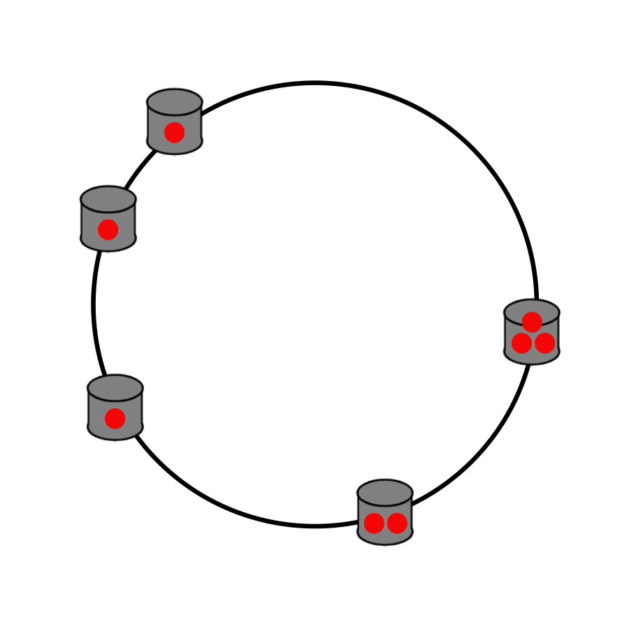
Consistent Hashing (CH) [1] is a widely adopted solution to this problem. In CH, objects and bins are both hashed to random locations on the unit circle. Objects are initially assigned to the closest bin in the clockwise direction (see Figure 1 and Section 2.2). CH is efficient for the dynamic setting because the addition or removal of a bin only affects the objects in the closest clockwise bin.
In practice, we cannot assign an unlimited number of objects to a bin without crashing the corresponding server. In [2], the authors address the problem by setting a maximum bin capacity , where objects are assigned to bins, each with a capacity parameter . Their hashing scheme ensures assigns new objects to the closest non-full bin in the clockwise direction and ensures that the maximum load is bounded by . There are also many hueristics, such as time-based expiry and eviction recommended in ASP.net [10], Microsoft [11], Mozilla [12].
Applications: Dynamic load assignment is a fundamental problem with a variety of concrete, practical applications. CH is a core part of Discord’s 250 million user chat app [13], Amazon’s Dynamo storage system [14] and Apache Cassandra, a distributed database system [15]. Google cloud and Vimeo video streaming both use CH with load bounds [16, 17]. CH is also used for information retrieval [18], distributed databases [19, 20, 21], and cloud systems [22, 23, 24]. Furthermore, CH resolves similar load-balancing issues that arise in peer-to-peer systems [25, 26], and content-addressable networks [27].
Our Contributions: We propose a new dynamic hashing algorithm with superior load balancing behavior. To minimize the risk of overloading a bin, all bins should ideally have approximately the same number of objects at all times. Existing algorithms experience a cascading effect that unevenly loads bins with the clockwise object assignment procedure.
Our algorithm improves upon the load balancing problem both in theory and practice. In our experiments on real user logs from the AOL search dataset and Indiana University Clicks dataset [28], the algorithm reduces cache misses by several orders of magnitude. We prove optimality for several criteria and show that the state-of-the-art method stochastically dominates the proposed method. The experiments and theory show that our algorithm provides the most even distribution of bin loads.
2 Background
2.1 2-Universal Hashing
A hash function is 2-universal if for all with , we have the following property for any ,
2.2 Consistent Hashing
In the CH scheme, objects and bins are hashed to random locations on the unit circle as shown in Figure 1(a). Objects are assigned to the closest bin in the clockwise direction, shown in Figure 1(b), with the final object bin assignment in Figure 1(c).
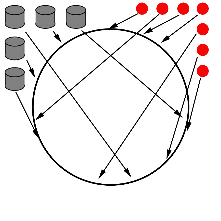
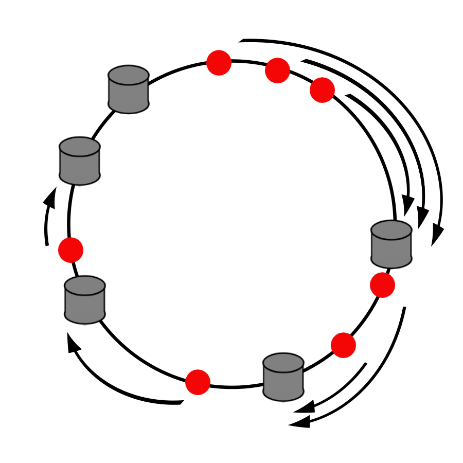
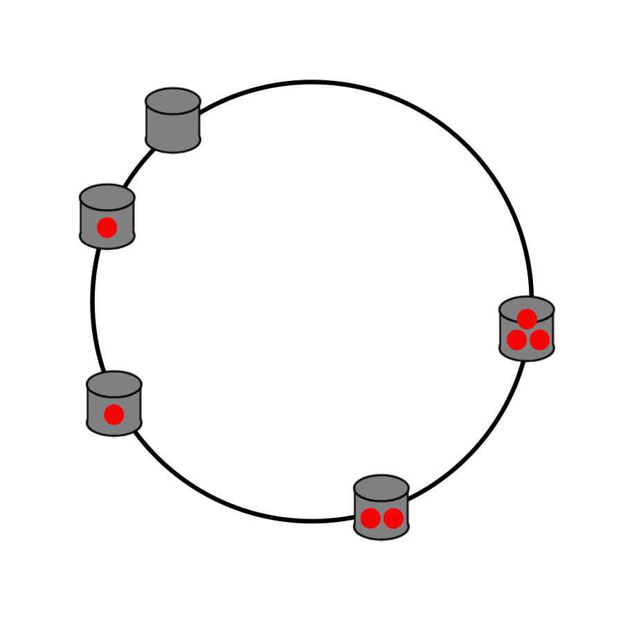
When a bin is removed, its objects are deposited into the next closest bin in the clockwise direction the next time they are requested. When a bin is added, it is used to cache incoming objects. Both procedures only reassign objects from one bin, unlike the naive hashing scheme. The arc length between a bin and its counter-clockwise neighbor determines the fraction of objects assigned to the bin. In expectation, the arc lengths are all the same because the bins are assigned to the circle via a randomized hash function. With equal arc lengths, each bin has the ideal load of . However, CH seldom provides ideal load balancing because the arc lengths have high variance.
2.3 Consistent Hashing with Bounded Loads
Consistent Hashing with Bounded Loads (CH-BL) was proposed by [2] to model bins with finite capacity. CH-BL extends CH with a maximum bin capacity . Here, is the number of objects, is the number of bins, and controls the bin capacity.
In CH-BL, if an object is about to be assigned to a full bin, it overflows or cascades into the nearest available bin in the clockwise direction. Figure 3 uses the bin object assignment from Figure 1 as the initial assignment with a maximum bin capacity of 3. A new object is hashed into the unit circle, but the closest bin in the clockwise direction is unavailable because it is full. Therefore, this object is assigned to the nearest available bin.
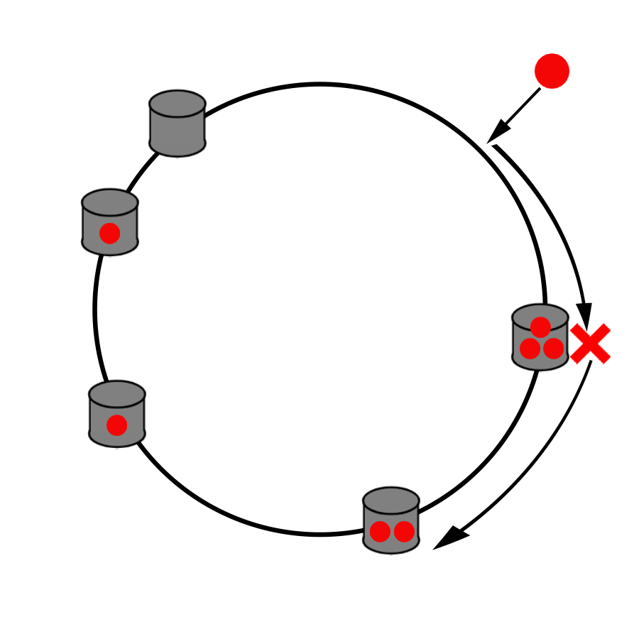

On bin removal, CH-BL performs the same reallocation procedure as CH, but with bounded loads. Objects from a deleted bin are cached in the closest available bin in the clockwise direction the next time the object is requested. Bin addition is handled the same as CH.
2.4 Cascaded Overflow of Consistent Hashing and Variants
CH-BL solves the bin capacity problem but introduces an overflow problem. Recall that the expected number of objects assigned to a particular bin is proportional to the bin’s arc length. As bins fill up in CH-BL, the nearest available (non-full) bin has a longer and longer effective arc length. The arc lengths for consecutive full bins add, causing the nearest available bin to fill faster. We call this phenomenon cascaded overflow.
Figure 3 shows cascaded overflow for the non-full bins in Figure 3 using the final object bin assignment in Figure 3 with a maximum bin capacity of 3. One bin now owns roughly 75% of the arc, so it will fill quickly while other bins are underutilized. The cascading effect creates an avalanche of overflowing bins that progressively cause the next bin to have an even larger arc length.
Cascaded overflow is a liability in practice because overloaded servers often fail and pass their loads to the nearest clockwise server. Cascaded overflow can trigger an avalanche of server failures as an enormous load bounces around the circle, crashing servers wherever it goes. In severe cases, this can bring down the entire service [5].
2.5 Simple Rehashing
At first glance, one reasonable approach is to rehash objects that map to a full bin rather than use the nearest clockwise bin. We reassign an object to bin rather than if bin is full. However, linear probing with random probes fails because it effectively rearranges the unit circle. Bin always overflows into , preserving the cascaded overflow effect.
3 Random Jump Consistent Hashing
Our proposal is motivated by Optimal Densification [29], a technique introduced to quickly compute minwise hashes in information retrieval. We break the cascade effect by introducing Random Jumps for Consistent Hashing (RJ-CH). In practice, the segments of the unit circle are mapped to an array. RJ-CH continuously rehashes objects until they reach an index associated with an available bin. Unlike simple rehashing, the RJ-CH hash function takes two arguments: the object and the failed attempts to find an available bin. The second argument breaks the cascading effect because it ensures that two objects have a low probability of overflowing to the same location. This probability is , where is the length of the array.
Figure 4(a) shows RJ-CH in a situation without full bins, which evolves into Figure 4(b) when a bin becomes full. RJ-CH prevents cascaded overflow because objects are assigned to any of the available bins with uniform probability by the universal hashing property. RJ-CH cannot be implemented with a dynamically changing array size, but this limitation is is common to RJ-CH, CH-BL and CH. We also note that load balancing methods are usually accompanied by hueristics like time-based expiry and eviction of stale objects [10, 11, 12] to evict duplicates and unused objects. Objects are commonly deleted when they are unused for some time. Many implementations, such as [10], impose stringent eviction criteria. It is also common practice to wipe the cache of a failed server and repopulate the cache as needed when the server is back online. RJ-CH is compatible with all such techniques, since deleting an element simply frees space in the bin.


3.1 Discussion: object removal, bin removal and bin addition schemes
When a bin is added, we may encounter a situation where an object is cached in the new bin while also existing somewhere else in the array. In practice, this is not a problem because the system will no longer request the duplicate and it will eventually be evicted by its bin. When a bin is removed, its objects will be cached in the available bin chosen by RJ-CH the next time the objects are requested.
4 Theoretical Analysis
In this section, we prove that the bin load under CH-BL stochastically dominates that of RJ-CH, showing that RJ-CH has lower bin load variance, fewer full bins and other desirable properties. In addition, the variance of CH-BL increases exponentially as bins become full. RJ-CH also achieves an algorithmic improvement over CH-BL for object insertion.
4.1 Bin load following CH-BL stochastically dominates RJ-CH
When reassignments are necessary, RJ-CH reassigns objects uniformly to the available bins, while CH-BL reassigns objects to the nearest clockwise bin. Even before a CH-BL bin fills, the object assignment probabilities are unequal as discussed in sections 4.3 and 4.4. Here, we assume that the CH-BL assignment probabilities are initially equal, corresponding to optimal initial bin placements. Let objects be assigned to bins with a maximum capacity . Our main theoretical result is as follows. It shows that RJ-CH is superior to CH-BL in terms of smaller variance of the number of objects in each bin, and in terms of the mean number of full bins. Detailed proofs are provided in the Appendix. The main result is as follows:
Theorem 1
Let ( ) denote the number of objects in bin when placing objects into a ring of bins with CH-BL or RJ-CH. Then,
| (1) |
Moreover,
| (2) |
where () is the number of full bins following the CH-BL (RJ-CH) method.
Theorem 2
Let be a convex function defined on . Then,
| (3) |
And the symmetry implies
| (4) |
The main idea of the proof of Theorem 2 is to consider a scheme where the first objects are assigned using CH-BL and the rest are assigned using RJ-CH. Such a scheme is worse than, stochastically dominates, a scheme where the first objects are assigned using CH-BL and the rest are assigned using RJ-CH. Only the th object of the two schemes follow a different assignment method. One key difficulty in the analysis lies in the fact that the differing assignment of that th object affects the assignment of the remaining objects. Lemma 1 proves an equivalent assignment method which allows the th object to be assigned last. Therefore, for the two schemes we only need to consider the "badness" of the last object, since all previous objects are assigned the same way. Lemmas 2, 3, 4 give us the assignment probability of that last object and tools to determine the stochastic dominance of the bin load of one scheme over the other. Lemma 5 completes the proof.
Lemma 1
Suppose bin already contains objects, with for . Distribute more objects into the bins in the following scheme indexed by : All objects are assigned uniformly to bins and relocated following RJ-CH, except for the -th object, which is assigned to bin 1, and reassigned following RJ-CH. Then, the final joint distribution of the numbers of objects in the bins will be the same regardless of the value of .
Consider again the scheme in which the first objects are assigned following CH-BL and the remaining objects are assigned following RJ-CH. The implication of Lemma 1 is given that the th object was assigned to a bin , it can equivalently be assigned as the th object to bin . If bin is full, then the object is reassigned using RJ-CH.
Denote the multinomial distribution for the number of objects in bins when assigning objects to bins where each object has probability of being assigned to bin . Let be the constrained multinomial distribution for the number of objects in bins when assigning objects to bins where each object has probability of being assigned to bin under the condition that each bin has at most objects. Let be the random number of objects in bin .
Lemma 2
If , the conditional distribution of subject to is where . Moreover, if , the conditional distribution of subject to is .
Lemma 2 can be understood as the distributions describing the results of assigning objects randomly to bins.
A random variable is stochastically smaller than , denoted as , if for all , or, equivalently, if for any bounded increasing function .
Lemma 3
Let , , be independent random binary random variables taking value 1 with probability and taking value 0 with probability . Assume . Let and . Then,
| (5) |
Moreover,
| (6) |
Consequently, and
| (7) |
If we know the assignment probability of a bin is greater than another, then Lemma 3 can be used to determine the stochastic dominance of the bin load of one bin over the other.
Lemma 4
Place objects into bins following CH-BL. Let be the number of objects in bins , and be the length of cluster of full bins to the right of bin , for . if the bin to the right hand side of bin is non-full. Let be all the non-full bins. Then, conditioning on , , and , follows the constrained multinomial distribution, i.e.,
| (8) |
where for , and .
Lemma 4 proves that in expectation bins on the left of longer clusters of full bins have more objects.
Lemma 5
Assign total objects into bins in a scheme with following three steps:
- 1.
Assign objects following CH-BL. Let denote all the non-full bins, with as the length of the cluster of full bins to the right of bin . For notational simplicity, assume .
- 2.
Assign one object into bins with probability , , such that and , and depends on only.
- 3.
Assign objects into the bins following RJ-CH.
Let be the numbers of objects in bins , and let be any convex function on . Then,
| (9) |
Proof of Theorem 2 In Lemma 5 if all are equal, Steps 1-3 are the same as assigning the first objects following CH-BL and rest objects following RJ-CH. If the first objects are assigned following CH-BL then , and the rest objects are assigned following RJ-CH. For the first scheme, we denote by as the final numbers of objects in bins . With this notation, are the final numbers of objects in bins by the latter method. Then, Lemma 5 proves that
for all . Hence,
| (10) |
Note that are the final numbers of objects in bins when all balls are distributed following RJ-CH, while are the final numbers of objects in bins when all balls are distributed following CH-BL. Therefore (10) implies (3).
4.2 Fewer bin searches
Bin searches are defined as the total number of bins (or servers) that must be searched to assign an object. It should be noted that this is not the total number of indexes in the array searched. We make this distinction because the latter tends to be implementation-specific. We will later provide experimental results for both metrics, but here we analyze object insertion as object removals in practice are taken care of by time-based decay and more stringent measures (Section 3.1). Let the number of bin searches be denoted as . Recall that there are objects, bins and a maximum capacity for some .
When inserting another object, CH-BL achieves the following upper bounds on the expected value of as a function of :
| (11) |
For RJ-CH, we assume a worst case scenario of bins full, and we prove the following theorem.
Theorem 3
Under RJ-CH, the expected value of is upper bounded by .
Observe that,
| (12) |
Setting a maximum capacity has a much greater impact for small and for small , RJ-CH is an order of a magnitude better. For large , RJ-CH is better. For slightly larger than 1, the methods are comparable. In practice, RJ-CH results in significantly fewer percentage of full bins which, in addition to the improved upper bound, results in an even more pronounced improvement in .
4.3 Expected number of objects until first overflow
Stateless addressing is one of the key requirements [5], which is that the assignment process should be independent of the number of objects in the non-full bins. Methods that, for example, always assign new objects to the bin with the least objects are not viable for consistent hashing because keeping track of object distribution in a dynamic environment is too slow and requires costly synchronization.
In this section, we look at the expected number of objects that can be assigned before any bins are full. If all bins have the same capacity, then lower expected number of objects indicates poor load balancing since one of the servers was overloaded prematurely. RJ-CH produces the uniform distribution which is optimal under stateless addressing [5]. Let be the number of objects assigned before any bin is full.
Theorem 4
Both the probability of no full bin and are maximized by the uniform distribution for all stateless addressing, which is achieved by RJ-CH.
4.4 Lower initial bin load variance
In this section we argue that even without the cascading effect, RJ-CH is still superior to the state-of-the-art. Recall that bin load is defined as the number of objects in a bin. Theorem 5 shows that RJ-CH minimizes bin load variance before the first full bin. This result applies over all distributions which satisfies the requirements of stateless addressing. Let be the random number of objects in bins and be the probability of an object being assigned to bin .
Theorem 5
Assume a fixed number of objects are assigned and no bins are full. is minimized by the uniform distribution for all stateless addressing, which is achieved by RJ-CH.
Cascaded overflow starts when we hit the first full bin. Theorem 5 suggests that even before the start of the cascading effect, CH has poor variance compared to RJ-CH. This is important as even heavily loaded servers are undesirable practically.
4.5 Object Assignment Probability Variance
We define the object assignment probability of a bin as the probability that a new object lands in that bin. Note that this probability is dependent on the previous object assignments seen so far, and hence is a random variable. We are concerned with the variance of the object assignment probability for the non-full bins. We will use to refer to the random probability that a new object lands in the non-full bin when there are full bins. It should be noted that when there are full bins and total bins, we have assignment probabilities. The variance of this random variable, or the object assignment probability variance, is a measure of load balancing performance. In the ideal case with perfect load balancing, all assignment probabilities should be the same and the variance should be zero. It follows from universal hashing that RJ-CH has this property, with . Therefore, we claim that RJ-CH is optimal in terms of this load balancing metric. CH-BL, on the other hand, has higher variance as it reassigns objects to the closest non-full bin in the clockwise direction. We obtain the following theorem:
Theorem 6
Assume that each non-full bin has an equal probability of being full. For CH-BL, strictly increases exponentially with rate at least for .
5 Experimental Evaluations
For evaluation, we provide both simulation results and results on real server logs.
5.1 Simulation results
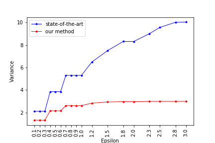
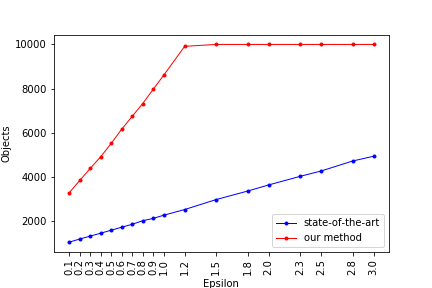
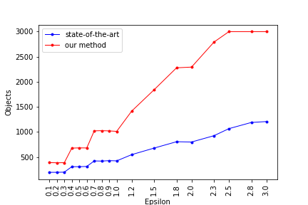
We generate objects and bins where each bin has capacity . We hash each of the bins into a large array, resolving bin collisions by rehashing. Bins are populated according to the two methods of RJ-CH and CH-BL. We sweep finely between 0.1 and 3, performing 1000 trials from scratch for each . We present results on percentage of bins full and wall clock time with 10000 objects and 1000 bins. Other results on variance of bin loads, bin searches, and objects till first full bin are given in Appendix L. Another setting with less load is given in Appendix R, and results are similar. Exact implementation details are given in Appendix M.


Figure 6 shows the percentage of bins that are full. For most , RJ-CH has a 20% - 40% lower percentage of total bins that are full. For the case of , only 25% of bins are full for RJ-CH as opposed to 60% for CH-BL. Clearly, this implies that CH-BL causes servers to overload earlier than required, indicating poor load balancing.
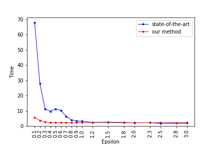
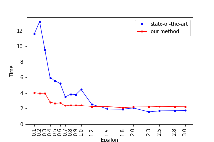
Empirical results on the wall clock time for inserting the th object are given in Figure 6. For wall clock time, RJ-CH attains between a 2x and 7x speedup for small . The speedup results from the fewer number of full bins, practical considerations of hashing, and the cascaded overflow of CH-BL.
5.2 AOL search logs experiments
In this section we present results with real AOL search logs. This is a dataset of user activity with 3,826,181 urls clicked, of which 607,782 are unique. We selected a wide range of configurations, Appendix K (Table 3), used in practice, such as reflecting the 80% of internet usage being video [30].
Definitions:
- •
- •
- •
Results are evaluated in cache misses, given in Table 2. Cache misses are presented as additional cache misses, since there is a large number of unavoidable cache misses for a given eviction time even with no server failures and infinite capacity. In all configurations, RJ-CH significantly decreases the number of cache misses by several orders of magnitude.
| Configuration | CH-BL | RJ-CH |
|---|---|---|
| Config 1 | 35780 | 312 |
| Config 2 | 52403 | 4680 |
| Config 3 | 12223 | 104 |
| Config 4 | 48571 | 9 |
| Configuration | CH-BL | RJ-CH |
|---|---|---|
| Config 1 | 72989 | 5549 |
| Config 2 | 98712 | 9054 |
| Config 3 | 105499 | 8641 |
| Config 4 | 49304 | 3498 |
5.3 Indiana University Clicks search logs experiments
In this section we present results using Indiana University Clicks search logs. This is a dataset of user activity, where we use the first 1,000,000 urls clicked of which 26,062 are unique. For this dataset, we again selected a wide range of configurations used in practice, given in Appendix K (Table 4).
Again, results are evaluated in cache misses, given in Table 2. In all configurations, RJ-CH significantly decreases the number of cache misses by roughly one order of magnitude.
6 Conclusion
From both theoretical and empirical results, RJ-CH significantly improves on the state-of-the-art for dynamic load balancing. With this method, objects are much more evenly distributed across bins and bins rarely hit maximum capacity. In terms of bin load, we also prove the stochastic dominance of CH-BL over RJ-CH and a corollary is RJ-CH has lower expected number of full bins and bin load variance. On the AOL search dataset and Indiana University Clicks dataset with real user data, RJ-CH reduces cache misses by several orders of magnitude.
7 Broader Impacts
CH is widely used in industry including the popular chat app Discord with over 250 million users [13], Amazon’s storage system Dynamo [14], the distributed database system Apache Cassandra [15], Google’s cloud system [16], Vimeo’s video streaming service [17], and many others. Improved CH has a direct and significant impact reducing energy consumption, improving the latency of the services, and reducing server costs due to the popularity and widespread use of the aforementioned services.
References
- [1] David Karger, Eric Lehman, Tom Leighton, Matthew Levine, Daniel Lewin, and Rina Panigraph. Consistent hashing and random trees: Distributed caching protocols for relieving hot spots on the world wide web. In Proceedings of the 29th Annual ACM Symposium on Theory of Computing, 1997.
- [2] Vahab Mirrokni, Mikkel Thorup, and Morteza Zadimoghaddam. Consistent hashing with bounded loads. SODA, 2018.
- [3] Ion Stoica, Robert Morris, David Karger, Frans Kaashoek, and Hari Balakrishnan. Chord: a scalable peer-to-peer lookup protocol for internet applications. ACM SIGCOMM Computer Communication Review, 2001.
- [4] Ion Stoica, Robert Morris, David Liben-Nowell, David Karger, Frans Kaashoek, Frank Dabek, and Hari Balakrishnan. Chord: a scalable peer-to-peer lookup protocol for internet applications. IEEE/ACM Trans. Netw., 2003.
- [5] Anshish Chawla, Benjamin Reed, Karl Juhnke, and Ghousuddin Syed. Semantics of caching with spoca: A stateless, proportional, optimally-consistent addressing algorithm. In USENIX ATM, 2011.
- [6] Dimitris Fotakis, Rasmus Pagh, Peter Sanders, and Paul G. Spirakis. Space efficient hash tables with worst case constant access time. Theory Comput. Syst., 2005.
- [7] Rasmus Pagh and Flemming Friche Rodler. Linear probing with constant independence. SIAM Journal on Computing, 2009.
- [8] Rasmus Pagh and Flemming Friche Rodler. Cuckoo hashing. Springer, 2001.
- [9] Rasmus Pagh and Flemming Friche Rodler. Cuckoo hashing. Journal of Algorithms, 2004.
- [10] Rick Anderson, John Luo, and Steve Smith. Cache in-memory in asp.net core. ASP.NET Core 3.0, 2019.
- [11] Alex Buck, Pedro Wood, Christopher Bennage, Peter Taylor, Tim Reilly, Tim Lovell-Smith, Alexey Sosnin, Nick Schonnig, Chris Voon, Duncan Mackenzie, Andrew Cook, and Marc Wilson. Caching best practices. Microsoft docs, 2017.
- [12] Caching. Mozilla docs, 2020.
- [13] Stanislav Vishnevskiy. How discord scaled elixir to 5,000,000 concurrent users. Discord Blog, 2017.
- [14] Giuseppe DeCandia, Deniz Hastorun, Madan Jampani, Gunavardhan Kakulapati, Avinash Lakshman, Alex Pilchin, Swaminathan Sivasubramanian, Peter Vosshall, and Werner Vogels. Dynamo: Amazon’s highly available key-value store. SOSP, 2007.
- [15] Avinash Lakshman and Prashant Malik. Cassandra: a decentralized structured storage system. ACM SIGOPS Operating Systems Review, 2010.
- [16] Vahab Mirrokni and Morteza Zadimoghaddam. Consistent hashing with bounded loads. Google Research Blog, 2017.
- [17] Andrew Rodland. Improving load balancing with a new consistent-hashing algorithm. Vimeo Engineering Blog, 2016.
- [18] David Grossman and Ophir Frieder. Information retrieval - algorithms and heuristics, second edition, volume 15 of the kluwer international series on information retrieval. Kluwer, 2004.
- [19] Tamer Ozsu and Patrick Valduriez. Principles of distributed database systems, third edition. Springer, 2011.
- [20] Josiah Carlson. Redis in action. Manning Publications Co., 2013.
- [21] Rajesh Nishtala, Hans Fugal, Steven Grimm, Marc Kwiatkowski, Herman Lee, Harry Li, Ryan McElroy, Mike Paleczny, Daniel Peek, Paul Saab, David Stafford, Tony Tung, and Venkateshwaran Venkataramani. Scaling memcache at facebook. In Proceedings of the 10th USENIX Conference on Networked Systems Design and Implementation, 2013.
- [22] David Karger, Alex Sherman, Andy Berkheimer, Bill Bogstad, Rizwan Dhanidina, Ken Iwamoto, Brian Kim, Luke Matkins, and Yoav Yerushalmi. Web caching with consistent hashing. Computer Networks, 1999.
- [23] Mitra Nasri and Mohsen Sharifi. Load balancing using consistent hashing: A real challenge for large scale distributed web crawlers. 23rd International Conference on Advanced Information Networking and Applications, 2009.
- [24] Xiaoming Wang and Dmitri Loguinov. Load-balancing performance of consistent hashing: Asymptotic analysis of random node join. IEEE/ACM Transactions on Networking, 2007.
- [25] Antony Rowstron and Peter Druschel. Pastry: Scalable, decentralized object location, and routing for large-scale peer-to-peer systems. Middleware, 2001.
- [26] Miguel Castro, Peter Druschel, Anne-Marie Kermarrec, and Antony IT Rowstron. Scribe: A large-scale and decentralized application-level multicast infrastructure. Selected Areas in Communications, IEEE, 2002.
- [27] Sylvia Ratnasamy, Paul Francis, Mark Handley, Richard Karp, and Scott Shenker. A scalable content-addressable network. ACM, 2001.
- [28] M. Meiss, F. Menczer, S. Fortunato, A. Flammini, and A. Vespignani. Ranking web sites with real user traffic. In Proc. First ACM International Conference on Web Search and Data Mining (WSDM), pages 65–75, 2008.
- [29] Anshumali Shrivastava. Optimal densification for fast and accurate minwise hashing. In International Conference on Machine Learning, 2017.
- [30] Cisco annual internet report (2018–2023) white paper. Cisco docs, 2020.
- [31] Tejas Karkhanis and J.E. Smith. A day in the life of a data cache miss. Workshop on Memory Performance Issues, 2002.
Appendix A Proof of Theorem 1
Appendix B Proof of Lemma 1
It suffices to show that, for two schemes indexed by and , the final joint distributions of the numbers of objects in the bins are the same. Let be the number of objects in bin 1 before the assignment of the th object. There are three cases.
Case 1. . The two schemes give same distribution of the th object and the th object. One will be assigned to bin 1 and the other uniformly distributed over the non-full bins before the th object has been assigned.
Case 2. . The two schemes give the same distribution of the th and th object. One object is added to bin 1 making it full and the other object is uniformly distributed over the rest of the non-full bins.
Case 3. . As bin 1 is full before the th object has been assigned, both schemes will distribute the th and th objects uniformly to the non-full bins, one after the other.
In summary, the two schemes give same joint distribution of the numbers of objects in bins after the th object has been assigned. Starting from th object, the two schemes are the same. As a result, the final joint distributions of the numbers of objects in bins will be the same for all schemes regardless of the value of the index . The proof is complete.
Appendix C Proof of Lemma 2
The distributions can be understood as the result of dropping objects into bins randomly. We omit the details.
Appendix D Proof of Lemma 3
Appendix E Proof of Lemma 4
For , consider objects been uniformly assigned into a cluster of bins , and reassigned according to the CH-BL. Denote as the probability that no objects are reassigned to beyond bin . In other words, is the probability that all objects are "self-contained" in bins under the CH-BL of relocation.
Fix values such that and . We consider the conditional distribution under the condition for some fixed , . Observe that . Write
The proof is complete.
Appendix F Proof of Lemma 5
There are two key observations. First, (9) is equivalent to minimization of , since the full bins in Step 1 will remain full till the end. Second, if we change Step 3 to "placing balls into bins in following RJ-CH", the distribution of will not change. We next argue that the distribution of will not change, if we change the entire distribution scheme in Steps 1-3 to Steps (a)-(c) in the following:
- 1.
same as Step 1.
- 2.
same as Step 3.
- 3.
same as Step 2, and reassigning following RJ-CH.
Steps (b) and (c) switch Steps 2 and 3. Unlike in Step 2, where the object need not be reassigned, in Step (c), the object may be assigned to a full bin and, in that case, reassigned following RJ-CH.
The equivalence of these two schemes of object assignment, one described in Steps 1-3 and one in Steps (a)-(c), in terms of the distribution of , can be understood by tracking the object in Step 2 and that in Step (c). Suppose in Step 2, the object is assigned to some bin . It follows from Lemma 3 that the final distribution of the numbers of objects in the bins will not change if the object in Step 2 is instead assigned as the last object into bin and reassigned following RJ-CH. Since both happen with same probability , the desired equivalence holds true. As a result, it suffices to prove (9) for the object distribution scheme in Steps (a)-(c).
Recall that are the non-full bins after Step (a). Let be all the non-full bins after Step (b) with denoting the number of objects in bin . Clearly . We show that, conditioning on and ,
| (16) |
where means stochastically smaller. For ease of notation and without loss of generality, let .
For simplicity of exposition, we only show the conditional stochastic dominance: . Let and be two nonnegative integers. Let , , be independent random variables taking values and , with probabilities such that for and for , where . Set and . Since , Lemma 2 implies that,
Now consider the condition that, in Step (a), there are a total of objects in bins and and in Step (b), there are a total of additional objects in bins and . It follows from Lemmas 1 and 4 that, under this condition, the conditional distribution of is the same as the conditional distribution of the above , under the condition that and . As a result, the conditional stochastic dominance of in (16) is proved.
Recall that we set for notational convenience. After Step (c), the number of objects in bin , , is
where and the conditioning is on . Here is the probability the last object is assigned to bin and is the probability the object is assigned to the full bins , with probability , then reassigned to bin .
Observe that, since is convex, is an increasing function of . Hence (16) implies is increasing in . Since , , are monotone increasing in , it follows that
where, in the last inequality, the equality holds when all are equal, i.e., . This inequality holds because the correlation of two sequences of increasing numbers is always nonnegative. Therefore, the conditional mean of is minimized when . Since are the final numbers of the objects in bins and the rest of the bins are already full after Step (b), we conclude that is minimized when are all equal. (9) is proved.
Appendix G Proof of Theorem 3
Recall that there are objects, bins, and capacity for some . Our claim is the RJ-CH method of assigning objects with uniform distribution to the non-full bins is expected to search bins to assign an object to a non-full bin in the worst case scenario. To show the upper bound, we assume the worst case scenario of bins full. Then,
| (17) |
The proof is complete.
Appendix H Proof of Theorem 4
Recall that there are objects, bins, and capacity for some . is the number of objects assigned before any bin is full. Our claim is the RJ-CH method of assigning objects with uniform distribution to the non-full bins maximizes both the probability no bin is full and .
For the binomial case where refers to bin 1 and refers to bin 2, is uniquely maximized by , where .
For the multinomial case, where and bins have probability :
If we consider the term then
with strict inequality when . Thus, for every pair of bin probabilities can be repeatedly replaced by their mean, and is then uniquely maximized by .
Recall that is the number of objects assigned before any bin is full.
Each term is maximized by the uniform distribution and the proof is complete.
Appendix I Proof of Theorem 5
To see that RJ-CH minimizes bin load variance before the first full bin, we only need to show that the conditional second moment of bin load is minimized by RJ-CH since the conditional mean is fixed as for each bin. Consider bins and . Let () be the random number of objects in bins () and () be the probability of objects being assigned to bin (). Assume for any fixed number . Under this condition, the conditional probability of an object assigned to given it is in or , is .
Suppose and are two random variables following binomial distributions with number of trials as and parameter as and respectively. Let and . Then for , and, if is even, . has an identical expression with . A key observation is that the ratio of the probability functions of and is increasing. Namely,
as a function of in the region is convex and increasing. It then follows that is stochastically greater than , i.e., , or, equivalently, for any .
Moreover, the monotone increasing ratio of probability functions of and also implies, for any , the conditional distribution of given and the conditional distribution of given still has a monotone increasing ratio of probability functions. Hence, the conditional distribution of given is still stochastically greater than the conditional distribution of given . As a result, for any increasing function . Choose , which is increasing in on . Then,
The above argument implies, conditioning on bins and having a total of objects, the conditional mean of is minimized by the uniform distribution.
Thus considering all bins, to minimize the bin load variance before the first full bin repeatedly replace every pair of bin probabilities by their mean. The proof is complete.
Appendix J Proof of Theorem 6 and a simulation
Recall that are random variables that represent probabilities where is the probability an object lands in the th non-full bin with full bins. Note that are identically distributed. There are total bins and for RJ-CH . We define the object assignment probability variance as . Clearly, for RJ-CH . The method of CH-BL reassigns objects that attempt to be assigned to a full bin to the closest non-full bin in the clockwise direction.
Let be the random variable that refers to the object assignment probability of the th bin to be full. Consider ,
Observe that,
and
We can write
Since and follow the same distribution, it follows that
As a result,
Therefore, we can see that the V term is given by
The E term is given by
Combining the two terms, we have
For , and for , . Therefore, strictly increases for and increases geometrically with rate at least for . The proof is complete.
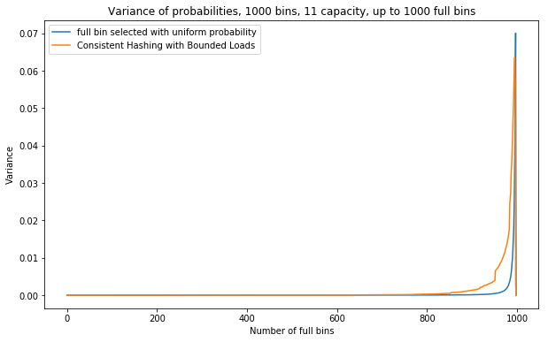
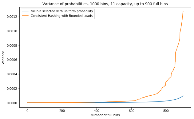
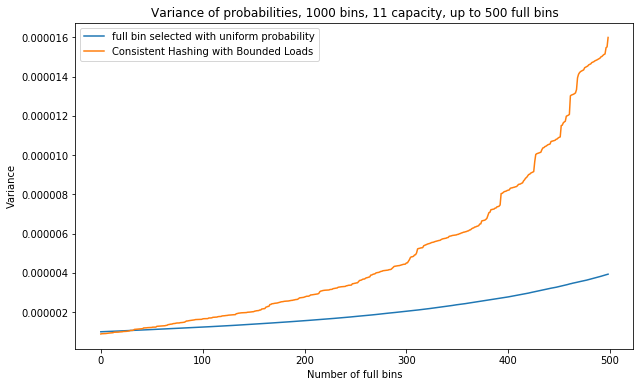
A simulation is given in Figure 7 where we also include CH-BL. The configuration for CH-BL is 1000 bins and capacity 11 (). We run 100 trials and take the mean. CH-BL performs significantly worse without the assumption that each non-full bin has equal probability of being the next full bin.
Appendix K AOL search logs and Indiana University Clicks configurations
Configurations for the AOL search dataset are given in Table 3. Configurations for the Indiana Clicks dataset are given in Table 4.
| Setting | Config 1 | Config 2 | Config 3 | Config 4 |
|---|---|---|---|---|
| Number of servers | 150 | 1000 | 100 | 20 |
| Cache size | 100 | 15 | 100 | 300 |
| Minutes for stale urls to be evicted | 300 | 300 | 120 | 120 |
| Minutes requests are served | 10 | 10 | 5 | 3 |
| Minutes for failed server to recover | 20 | 10 | 10 | 10 |
| Number of concurrent requests till server failure | 50 | 15 | 50 | 500 |
| Setting | Config 1 | Config 2 | Config 3 | Config 4 |
|---|---|---|---|---|
| Number of servers | 500 | 1000 | 800 | 200 |
| Cache size | 500 | 300 | 300 | 3000 |
| Minutes for stale urls to be evicted | 30 | 120 | 15 | 30 |
| Minutes requests are served | 5 | 5 | 5 | 3 |
| Minutes for failed server to recover | 10 | 10 | 7 | 15 |
| Number of concurrent requests till server failure | 2000 | 1000 | 1000 | 5000 |
Appendix L Additional simulation results
We generate objects and bins where each bin has capacity . We hash each of the bins into a large array, resolving bin collisions by rehashing. Bins are populated according to the two methods of RJ-CH and CH-BL.
We present results here with 10000 objects and 1000 bins, and also show results with less load, 3000 objects and 1000 bins, in Appendix R. Results in this different setting are similar. We draw attention to the 10000 objects, 1000 bins case as low object bin ratios tend to be easier in practice. However, even in a 1:1 object to bin ratio, we observe that RJ-CH achieves superior load balance. The larger the object to bin ratio, the better RJ-CH is in comparison.
We also performed the same simulations allowing objects and bins to arrive and leave. After placing all objects, objects and bins arrive and leave at a rate of of objects to bins. We then observe the load balancing metrics after objects have arrived or left. The results with such a methodology are similar to the previously introduced simulation methodology and we omit these results for succinctness. For additional experiments with a variety of combinations of configurations, see Appendix R. For implementation details, see Appendix M.
L.1 Variance of bin loads
| Variance of bin loads | Percentage of bins full | |||||||
| CH-BL mean | std | RJ-CH mean | std | CH-BL mean | std | RJ-CH mean | std | |
| 0.1 | 6.8 | 0.2 | 2.6 | 0.1 | 0.837 | 0.006 | 0.626 | 0.010 |
| 0.3 | 19.1 | 0.4 | 6.6 | 0.2 | 0.602 | 0.009 | 0.250 | 0.010 |
| 1 | 51.9 | 1.2 | 10.0 | 0.4 | 0.224 | 0.009 | 0.003 | 0.002 |
| 3 | 95.0 | 3.6 | 10.0 | 0.5 | 0.024 | 0.004 | 0.000 | 0.000 |
Recall that bin load is defined as the number of objects in a bin. Figure 9 shows the variance of bin loads against for different object bin configurations. A small variance is an indicator of better load balancing. RJ-CH achieves a 3x-10x improvement in bin load variance for small and large , with tabulated data in Table 5.
L.2 Bin searches
Recall that bin search is defined as the number of bins searched. Figure 9 shows the bin searches for the th object to be assigned after objects and bins have already been placed. Large is uninteresting for this case as there will be very few full bins. For interesting , RJ-CH achieves a staggering 10x-25x improvement in bin searches.


L.3 Percentage of bins full
Figure 6 shows the percentage of bins that are full. For most , RJ-CH has a 20% - 40% lower percentage of total bins that are full. For the case of , only 25% of bins are full for RJ-CH as opposed to 60% for CH-BL, given in Table . Clearly, this implies that CH-BL causes servers to overload earlier than required, indicating poor load balancing.
L.4 Objects till first full bin
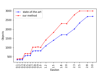
Figure 11 shows the number of objects that are assigned before a bin is full. This number indicates the amount of load the system can tolerate before observing an overloaded server. RJ-CH achieves a 3x-5x improvement in the number of objects until one bin is full for both small and large .

L.5 Steps and wall clock time
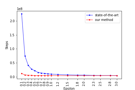
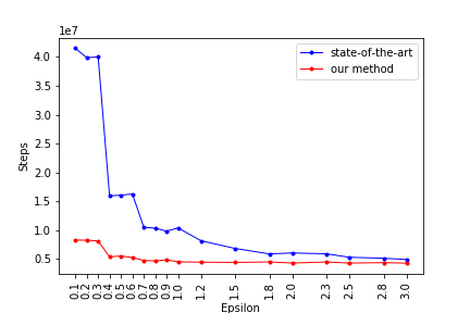
Here we present empirical results on the total steps and wall clock time for inserting the th object. Recall that objects are assigned to bins in a large array. We define two metrics - total number of steps and the total wall clock time. A step is defined as one index search in the array regardless of whether or not a bin exists at that index.
For inserting the th object, RJ-CH achieves as much as 20x speedup in total steps. For wall clock time, RJ-CH attains between a 2x and 7x speedup for smaller values of . The speedup in wall clock time is attributed to the fewer number of full bins, practical considerations of hashing, and the cascaded overflow of CH-BL.

Appendix M Implementation details
We use a roughly 1000 sparse array of size and the hash function Murmurhash. For each trial, we generate a pseudo-random initial string to represent each object and bin. For RJ-CH, whenever an object or bin is hashed into the array, we initialize a new counter with value 0 which is incremented until the object or bin is placed. On each iteration, the counter is converted to a string and concatenated to the pseudo-random initial string as input to Murmurhash, which produces a 128 bit number. The number is split up into four 32 bit numbers to generate the next array indexes. For an array of size , we use the first 20 bits of each 32 bit hash code. For CH-BL, we generate the initial array index using Murmurhash and increment the index to walk along the array. For wall clock time and total steps, we map the array to an array of size before measuring object insertion. A single thread is used for simulations. We note that there may be benefits of running in parallel.
Appendix N Discussion: Biased hash functions
In practice, hash functions do not hash inputs to all possible outputs with equal probability. We can imagine a very biased hash function that outputs a number with 90% probability and all other possible outputs with equal probability. This would clearly be very damaging to CH-BL. After the closest bin in the clockwise direction is full, the cascading effect will be severe. On the other hand, for RJ-CH if a bin exists at that index, after it is full RJ-CH recovers the uniform distribution of assigning objects to bins. In practice, hash functions are not nearly that biased, but we still make the below general observations about robustness against biased hash functions:
1. After the bins in the biased regions of the array are full, RJ-CH recovers the uniform distribution. CH-BL continues to worsen with the cascading effect.
2. Given that no bins are hashed into the biased regions of the array, RJ-CH recovers the uniform distribution. For CH-BL, the closest clockwise bin is severely affected.
Appendix O Tabulated simulation results
Simulation results in the main manuscript in tabulated form in Tables O, O, O, O. A virtual bin is a virtual copy of a bin that is a reference to the bin but is in a different index in the array.
| objects | bins | epsilon | virtual bins | CH-BL mean | std | RJ-CH mean | std |
|---|---|---|---|---|---|---|---|
| 10000 | 1000 | 0.1 | 0 | 6.8 | 0.2 | 2.6 | 0.1 |
| 10000 | 1000 | 0.3 | 0 | 19.1 | 0.4 | 6.6 | 0.2 |
| 10000 | 1000 | 1 | 0 | 51.9 | 1.2 | 10.0 | 0.4 |
| 10000 | 1000 | 3 | 0 | 95.0 | 3.6 | 10.0 | 0.5 |
| 10000 | 1000 | 0.1 | log(k) | 3.6 | 0.14 | 2.6 | 0.10 |
| 10000 | 1000 | 0.3 | log(k) | 10.0 | 0.29 | 6.6 | 0.22 |
| 10000 | 1000 | 1 | log(k) | 21.4 | 0.77 | 10.0 | 0.44 |
| 10000 | 1000 | 3 | log(k) | 24.2 | 1.16 | 10.0 | 0.46 |
| 3000 | 1000 | 0.1 | 0 | 2.1 | 0.04 | 1.3 | 0.04 |
| 3000 | 1000 | 0.3 | 0 | 2.1 | 0.04 | 1.3 | 0.04 |
| 3000 | 1000 | 1 | 0 | 5.3 | 0.11 | 2.6 | 0.09 |
| 3000 | 1000 | 3 | 0 | 10.0 | 0.36 | 3.0 | 0.13 |
| 3000 | 1000 | 0.1 | log(k) | 1.5 | 0.04 | 1.3 | 0.04 |
| 3000 | 1000 | 0.3 | log(k) | 1.5 | 0.04 | 1.3 | 0.04 |
| 3000 | 1000 | 1 | log(k) | 3.2 | 0.10 | 2.6 | 0.09 |
| 3000 | 1000 | 3 | log(k) | 4.3 | 0.20 | 3.0 | 0.13 |
| objects | bins | epsilon | virtual bins | CH-BL mean | std | RJ-CH mean | std |
|---|---|---|---|---|---|---|---|
| 10000 | 1000 | 0.1 | 0 | 51.52 | 68.01 | 2.79 | 2.26 |
| 10000 | 1000 | 0.3 | 0 | 9.31 | 11.34 | 1.31 | 0.65 |
| 10000 | 1000 | 1 | 0 | 2.19 | 1.76 | 1.01 | 0.09 |
| 10000 | 1000 | 3 | 0 | 1.12 | 0.38 | 1.00 | 0.00 |
| 10000 | 1000 | 0.1 | log(k) | 4.00 | 3.44 | 2.66 | 2.21 |
| 10000 | 1000 | 0.3 | log(k) | 1.82 | 1.28 | 1.33 | 0.68 |
| 10000 | 1000 | 1 | log(k) | 1.08 | 0.30 | 1.00 | 0.04 |
| 10000 | 1000 | 3 | log(k) | 1.00 | 0.03 | 1.00 | 0.00 |
| 3000 | 1000 | 0.1 | 0 | 10.34 | 14.06 | 1.95 | 1.36 |
| 3000 | 1000 | 0.3 | 0 | 9.48 | 11.85 | 1.90 | 1.30 |
| 3000 | 1000 | 1 | 0 | 2.35 | 2.13 | 1.08 | 0.30 |
| 3000 | 1000 | 3 | 0 | 1.17 | 0.46 | 1.00 | 0.00 |
| 3000 | 1000 | 0.1 | log(k) | 2.26 | 1.74 | 1.88 | 1.29 |
| 3000 | 1000 | 0.3 | log(k) | 2.32 | 1.71 | 1.90 | 1.31 |
| 3000 | 1000 | 1 | log(k) | 1.24 | 0.52 | 1.10 | 0.33 |
| 3000 | 1000 | 3 | log(k) | 1.00 | 0.05 | 1.00 | 0.00 |
| objects | bins | epsilon | virtual bins | CH-BL mean | std | RJ-CH mean | std |
|---|---|---|---|---|---|---|---|
| 10000 | 1000 | 0.1 | 0 | 1062 | 230 | 3295 | 477 |
| 10000 | 1000 | 0.3 | 0 | 1335 | 227 | 4392 | 579 |
| 10000 | 1000 | 1 | 0 | 2277 | 410 | 8606 | 852 |
| 10000 | 1000 | 3 | 0 | 4945 | 832 | 10000 | nan |
| 10000 | 1000 | 0.1 | log(k) | 2342 | 389 | 3303 | 495 |
| 10000 | 1000 | 0.3 | log(k) | 3027 | 447 | 4371 | 557 |
| 10000 | 1000 | 1 | log(k) | 5480 | 724 | 8638 | 828 |
| 10000 | 1000 | 3 | log(k) | 10000 | nan | 10000 | nan |
| 3000 | 1000 | 0.1 | 0 | 194 | 63 | 388 | 117 |
| 3000 | 1000 | 0.3 | 0 | 197 | 63 | 387 | 116 |
| 3000 | 1000 | 1 | 0 | 422 | 112 | 1011 | 227 |
| 3000 | 1000 | 3 | 0 | 1206 | 238 | 3000 | nan |
| 3000 | 1000 | 0.1 | log(k) | 331 | 104 | 378 | 116 |
| 3000 | 1000 | 0.3 | log(k) | 331 | 102 | 395 | 113 |
| 3000 | 1000 | 1 | log(k) | 816 | 186 | 1006 | 224 |
| 3000 | 1000 | 3 | log(k) | 3000 | nan | 3000 | nan |
| objects | bins | epsilon | virtual bins | CH-BL mean | std | RJ-CH mean | std |
|---|---|---|---|---|---|---|---|
| 10000 | 1000 | 0.1 | 0 | 0.837 | 0.006 | 0.626 | 0.010 |
| 10000 | 1000 | 0.3 | 0 | 0.602 | 0.009 | 0.250 | 0.010 |
| 10000 | 1000 | 1 | 0 | 0.224 | 0.009 | 0.003 | 0.002 |
| 10000 | 1000 | 3 | 0 | 0.024 | 0.004 | 0.000 | 0.000 |
| 10000 | 1000 | 0.1 | log(k) | 0.699 | 0.009 | 0.626 | 0.009 |
| 10000 | 1000 | 0.3 | log(k) | 0.377 | 0.010 | 0.249 | 0.010 |
| 10000 | 1000 | 1 | log(k) | 0.046 | 0.006 | 0.003 | 0.002 |
| 10000 | 1000 | 3 | log(k) | 0.000 | 0.000 | 0.000 | 0.000 |
| 3000 | 1000 | 0.1 | 0 | 0.622 | 0.008 | 0.472 | 0.010 |
| 3000 | 1000 | 0.3 | 0 | 0.622 | 0.008 | 0.473 | 0.009 |
| 3000 | 1000 | 1 | 0 | 0.271 | 0.009 | 0.089 | 0.008 |
| 3000 | 1000 | 3 | 0 | 0.035 | 0.005 | 0.000 | 0.000 |
| 3000 | 1000 | 0.1 | log(k) | 0.506 | 0.009 | 0.473 | 0.009 |
| 3000 | 1000 | 0.3 | log(k) | 0.507 | 0.009 | 0.473 | 0.009 |
| 3000 | 1000 | 1 | log(k) | 0.133 | 0.008 | 0.089 | 0.007 |
| 3000 | 1000 | 3 | log(k) | 0.001 | 0.001 | 0.000 | 0.000 |
Appendix P Tabulated simulation results for dynamic simulation
We performed the same simulations with dynamic objects and bins to compare CH-BL with RJ-CH. After placing all objects, objects and bins arrive and leave at a rate of of objects to bins. We then observe the load balance metrics after objects have arrived or left. Results given in Tables P, P, P. A virtual bin is a virtual copy of a bin that is a reference to the bin but is in a different index in the array.
| objects | bins | rate | epsilon | virtual bins | CH-BL mean | std | RJ-CH mean | std |
|---|---|---|---|---|---|---|---|---|
| 10000 | 1000 | 0.1 | 0 | 7.1 | 1.92 | 2.6 | 0.77 | |
| 10000 | 1000 | 0.3 | 0 | 19.1 | 1.32 | 6.6 | 0.39 | |
| 10000 | 1000 | 1 | 0 | 51.9 | 1.39 | 10.0 | 0.52 | |
| 10000 | 1000 | 3 | 0 | 95.1 | 6.26 | 10.0 | 0.56 | |
| 10000 | 1000 | 0.1 | log(k) | 4.0 | 0.94 | 2.63 | 0.82 | |
| 10000 | 1000 | 0.3 | log(k) | 10.1 | 0.61 | 6.51 | 0.43 | |
| 10000 | 1000 | 1 | log(k) | 21.4 | 1.00 | 9.89 | 0.53 | |
| 10000 | 1000 | 3 | log(k) | 24.3 | 1.66 | 10.07 | 0.47 |
| objects | bins | rate | epsilon | virtual bins | CH-BL mean | std | RJ-CH mean | std |
|---|---|---|---|---|---|---|---|---|
| 10000 | 1000 | 0.1 | 0 | 60.05 | 102.57 | 2.44 | 2.09 | |
| 10000 | 1000 | 0.3 | 0 | 10.45 | 11.94 | 1.31 | 0.59 | |
| 10000 | 1000 | 1 | 0 | 2.17 | 1.65 | 1.00 | 0.00 | |
| 10000 | 1000 | 3 | 0 | 1.23 | 0.53 | 1.00 | 0.00 | |
| 10000 | 1000 | 0.1 | log(k) | 4.17 | 5.26 | 2.96 | 2.89 | |
| 10000 | 1000 | 0.3 | log(k) | 1.87 | 1.55 | 1.32 | 0.68 | |
| 10000 | 1000 | 1 | log(k) | 1.07 | 0.32 | 1.01 | 0.99 | |
| 10000 | 1000 | 3 | log(k) | 1.00 | 0.00 | 1.00 | 0 |
| objects | bins | rate | epsilon | virtual bins | CH-BL mean | std | RJ-CH mean | std |
|---|---|---|---|---|---|---|---|---|
| 10000 | 1000 | 0.1 | 0 | 0.828 | 0.050 | 0.626 | 0.099 | |
| 10000 | 1000 | 0.3 | 0 | 0.601 | 0.041 | 0.249 | 0.046 | |
| 10000 | 1000 | 1 | 0 | 0.224 | 0.021 | 0.004 | 0.002 | |
| 10000 | 1000 | 3 | 0 | 0.025 | 0.005 | 0.000 | 0.000 | |
| 10000 | 1000 | 0.1 | log(k) | 0.688 | 0.072 | 0.630 | 0.106 | |
| 10000 | 1000 | 0.3 | log(k) | 0.378 | 0.045 | 0.250 | 0.047 | |
| 10000 | 1000 | 1 | log(k) | 0.046 | 0.011 | 0.004 | 0.003 | |
| 10000 | 1000 | 3 | log(k) | 0.000 | 0.000 | 0.000 | 0.000 |
Appendix Q Simulation comparison between Consistent Hashing with Bounded Loads with and without re-hashing on every full bin
Here we provide empirical results showing the similar performance between CH-BL and the direct extension of CH-BL where objects are re-hashing upon encountering a full bin. Note that for objects placed until first full bin both methods are equivalent as re-hashing does not occur until there is a full bin. For the other measures, the two methods are comparable.
| objects | bins | epsilon | virtual bins | CH-BL mean | std | re-hashing mean | std |
|---|---|---|---|---|---|---|---|
| 10000 | 1000 | 0.1 | 0 | 6.8 | 0.2 | 6.7 | 0.2 |
| 10000 | 1000 | 0.3 | 0 | 19.1 | 0.4 | 19.2 | 0.4 |
| 10000 | 1000 | 1 | 0 | 51.9 | 1.2 | 52.1 | 1.1 |
| 10000 | 1000 | 3 | 0 | 95.0 | 3.6 | 95.1 | 3.7 |
| 10000 | 1000 | 0.1 | log(k) | 3.6 | 0.14 | 3.8 | 0.15 |
| 10000 | 1000 | 0.3 | log(k) | 10.0 | 0.29 | 10.1 | 0.29 |
| 10000 | 1000 | 1 | log(k) | 21.4 | 0.77 | 21.2 | 0.78 |
| 10000 | 1000 | 3 | log(k) | 24.2 | 1.16 | 24.2 | 1.17 |
| objects | bins | epsilon | virtual bins | CH-BL mean | std | re-hashing mean | std |
|---|---|---|---|---|---|---|---|
| 10000 | 1000 | 0.1 | 0 | 51.52 | 68.01 | 70.55 | 74.24 |
| 10000 | 1000 | 0.3 | 0 | 9.31 | 11.34 | 9.19 | 8.71 |
| 10000 | 1000 | 1 | 0 | 2.19 | 1.76 | 2.21 | 1.57 |
| 10000 | 1000 | 3 | 0 | 1.12 | 0.38 | 1.13 | 0.38 |
| 10000 | 1000 | 0.1 | log(k) | 4.00 | 3.44 | 5.28 | 4.58 |
| 10000 | 1000 | 0.3 | log(k) | 1.82 | 1.28 | 2.08 | 1.52 |
| 10000 | 1000 | 1 | log(k) | 1.08 | 0.30 | 1.09 | 0.29 |
| 10000 | 1000 | 3 | log(k) | 1.00 | 0.03 | 1.00 | 0.00 |
| objects | bins | epsilon | virtual bins | CH-BL mean | std | re-hashing mean | std |
|---|---|---|---|---|---|---|---|
| 10000 | 1000 | 0.1 | 0 | 0.837 | 0.006 | 0.836 | 0.006 |
| 10000 | 1000 | 0.3 | 0 | 0.602 | 0.009 | 0.603 | 0.009 |
| 10000 | 1000 | 1 | 0 | 0.224 | 0.009 | 0.223 | 0.009 |
| 10000 | 1000 | 3 | 0 | 0.024 | 0.004 | 0.024 | 0.004 |
| 10000 | 1000 | 0.1 | log(k) | 0.699 | 0.009 | 0.714 | 0.009 |
| 10000 | 1000 | 0.3 | log(k) | 0.377 | 0.010 | 0.389 | 0.009 |
| 10000 | 1000 | 1 | log(k) | 0.046 | 0.006 | 0.046 | 0.006 |
| 10000 | 1000 | 3 | log(k) | 0.000 | 0.000 | 0.000 | 0.000 |
| objects | bins | epsilon | virtual bins | CH-BL mean | std | re-hashing mean | std |
|---|---|---|---|---|---|---|---|
| 10000 | 1000 | 0.1 | 0 | 230 | 300 | 296 | 300 |
| 10000 | 1000 | 0.3 | 0 | 41 | 60 | 44 | 40 |
| 10000 | 1000 | 1 | 0 | 9.7 | 10 | 9.6 | 10 |
| 10000 | 1000 | 3 | 0 | 4.4 | 5.0 | 4.7 | 6.0 |
| 10000 | 1000 | 0.1 | log(k) | 2.4 | 3.0 | 3.4 | 4.0 |
| 10000 | 1000 | 0.3 | log(k) | 1.1 | 1.0 | 1.2 | 1.0 |
| 10000 | 1000 | 1 | log(k) | 0.7 | 0.7 | 0.7 | 0.7 |
| 10000 | 1000 | 3 | log(k) | 0.6 | 0.6 | 0.6 | 0.7 |
Appendix R Comparison for virtual bins and supplementary figures
We generate objects and bins with virtual copies of each bin where each bin has capacity . A virtual copy of a bin is a reference to the bin that is in a different index in the array. Virtual bins may be used to improve wall clock time. We hash each of the bins into a large array with few collisions. We then populate the bins according to the two methods of RJ-CH and CH-BL. We resolve bin collisions by rehashing. We note here that virtual copies can be undesirable due to bin collisions, especially when the total number of bins is large.
We use the pairs (1000 objects, 1000 bins), and (3000 objects, 1000 bins). For each pair, we use no virtual bins or virtual bins. We try all , and perform 1000 trials for each pair and where we initialize each trial from scratch.