Jeffery orbits in shear-thinning fluids

We consider here a prolate spheroid $\mathcal{B}$ with surface $\partial\mathcal{B}$, whose axis of symmetry is defined by the unit vector $\mathbf{p}$ as shown in Fig. 1. The polar angle of the particle, with respect to a fixed lab frame whose origin is at the particle center, is $\theta$ while $\phi$ is the azimuthal angle. The major (minor) axis length is denoted by $a$ $(b)$ and the aspect ratio is $\lambda=a/b=1/{\sqrt{1-e^{2}}}>1$. The spheroid is immersed in an otherwise linear velocity field defined by $\mathbf{u}^{\infty}=\mathbf{A}^{\infty}\cdot\mathbf{x}$, whose origin is at the center of the particle to eliminate any constant translation. The velocity gradient tensor $\boldsymbol{\nabla}\mathbf{u}^{\infty}=\mathbf{A}^{\infty}$ is constant and may be decomposed in the usual way into symmetric and antisymmetric parts $\mathbf{A}^{\infty}=\mathbf{E}^{\infty}+\mathbf{\Omega}^{\infty}\times\mathbf{I}$ where $\mathbf{\Omega}^{\infty}$ is the angular velocity of the background flow ($\mathbf{I}$ is the identity). The flow-shear plane is defined by the basis $\mathbf{e}_{x}$, and $\mathbf{e}_{y}$.

Given a fluid velocity field $\mathbf{u}$, we define a disturbance velocity field relative to the background as

We assume no slip on the surface of the spheroid and that the disturbance flow is zero far from the spheroid, written in terms of the disturbance quantities the boundary conditions are

where $\mathbf{\Omega}$ is the angular velocity of the spheroid (the translation velocity $\mathbf{U}=\mathbf{0}$ by construction). The difference in the angular velocity of the spheroid and the undisturbed background flow $\mathbf{\Omega}^{\prime}=\mathbf{\Omega}-\mathbf{\Omega}^{\infty}$ is sometimes referred to as the slip angular velocity Einarsson et al. 2015b (although the no-slip condition is indeed satisfied). The evolution of the particle director is

We consider here fluids that shear thin, meaning the viscosity of the fluids, $\eta$, decreases with increasing strain rates, $\dot{\boldsymbol{\gamma}}$. To capture this behavior and its effect on the dynamics of a prolate ellipsoid in shear we use the Carreau model Bird et al. 1987 for a generalized Newtonian fluid with deviatoric stress

where the functional dependence of the viscosity on the strain-rate,

is characterized by a zero-shear viscosity $\eta_{0}$, an infinite-shear viscosity $\eta_{\infty}$, a time constant $\lambda_{t}$, and a power-law index $n<1$. The magnitude of strain-rate is defined $|\dot{\gamma}|=\sqrt{\dot{\boldsymbol{\gamma}}:\dot{\boldsymbol{\gamma}}}$. In this study, we explore only the weakly shear-thinning effects on the dynamics of the particle. In this regard, we always assume that $\lambda_{t}\ll 1/\dot{\gamma}_{c}$, where we define $\dot{\gamma}_{c}\equiv\sqrt{2\mathbf{E}^{\infty}:\mathbf{E}^{\infty}}$ as the characteristic strain rate of the flow defined by the external imposed flow. The deviatoric stress may be conveniently decomposed into Newtonian and non-Newtonian parts, $\boldsymbol{\tau}=\eta_{0}\dot{\boldsymbol{\gamma}}+\boldsymbol{\tau}_{NN}$ where the non-Newtonian part,

is defined as the amount of shear thinning relative to the zero-shear viscosity $\eta_{0}$.

In the absence of inertia, the velocity of a particle in a background flow of a fluid of arbitrary rheology may be written as

where $\mathsf{\mathsfbfit U}=\left[\mathbf{U}\ \mathbf{\Omega}\right]^{\top}$ is a 6-dimensional vectors containing translational and rotational velocities, likewise $\mathsf{\mathsfbfit F}=\left[\mathbf{F}\ \mathbf{L}\right]^{\top}$ represents both force and torque Elfring 2017. We consider here a particle that is neutrally buoyant and that no other external force acts on the particle and thus $\mathsf{\mathsfbfit F}_{ext}=\mathbf{0}$.

The term

is the drag force and torque on a particle held fixed in a background flow $\mathbf{u}^{\infty}$ of a Newtonian fluid of constant viscosity $\eta_{0}$. In a Newtonian fluid this force, along with the rigid-body resistance tensor,

for the particle in the same Newtonian fluid, would entirely determine the dynamics of a freely moving particle $\mathsf{\mathsfbfit U}_{0}=\mathsf{\mathsfbfit{\hat{R}}}_{\mathsf{\mathsfbfit F}\mathsf{\mathsfbfit U}}^{-1}\cdot\mathsf{\mathsfbfit F}_{T}$.

In a non-Newtonian fluid, there is an extra force/torque on the particle due to the extra deviatoric stress $\boldsymbol{\tau}_{NN}$ in the fluid volume $\mathcal{V}$ in which the particle is immersed Leal 1980. This force given by

We may write for simplicity that velocity is composed of a Newtonian part and a non-Newtonian correction $\mathsf{\mathsfbfit U}=\mathsf{\mathsfbfit U}_{0}+\mathsf{\mathsfbfit{\hat{R}}}_{\mathsf{\mathsfbfit F}\mathsf{\mathsfbfit U}}^{-1}\cdot\mathsf{\mathsfbfit F}_{NN}$. A similar approach has also been used for studying the dynamics of active particles in complex fluids (Lauga 2009; Natale et al. 2017; Elfring 2017).

The tensors $\mathsf{\mathsfbfit{\hat{E}}}_{\mathsf{\mathsfbfit U}}$ and $\mathsf{\mathsfbfit{\hat{T}}}_{\mathsf{\mathsfbfit U}}$, in addition to $\mathsf{\mathsfbfit{\hat{R}}}_{\mathsf{\mathsfbfit F}\mathsf{\mathsfbfit U}}$, are linear operators that are calculated from the resistance problem for the same particle in a Newtonian fluid with viscosity $\eta_{0}$. The tensors $\mathsf{\mathsfbfit{\hat{E}}}_{\mathsf{\mathsfbfit U}}$ and $\mathsf{\mathsfbfit{\hat{T}}}_{\mathsf{\mathsfbfit U}}$ are functions of position in space that map the rigid-body motion $\hat{\mathsf{\mathsfbfit U}}$ of a particle to the fluid strain-rate $\hat{{\dot{\boldsymbol{\gamma}}}}=2\mathsf{\mathsfbfit{\hat{E}}}_{\mathsf{\mathsfbfit U}}\cdot\mathsf{\mathsfbfit{\hat{U}}}$ and stress fields $\hat{\boldsymbol{\sigma}}=\mathsf{\mathsfbfit{\hat{T}}}_{\mathsf{\mathsfbfit U}}\cdot\mathsf{\mathsfbfit{\hat{U}}}$, respectively.

In our study the translational velocity of the particle is zero, $\mathbf{U}=\mathbf{0}$, and by symmetry the only relevant component of the hydrodynamic resistance is $\hat{\mathbf{R}}_{\mathbf{L}\mathbf{\Omega}}$. Because of this the above general expressions simplify considerably so that the angular velocity of the particle in a non-Newtonian fluid is

where the angular velocity in a Newtonian fluid

Clearly, the Newtonian dynamics are well known, and to determine the correction we must (only) resolve the integral on the right-hand side of (12). The tensors $\hat{\mathbf{R}}_{\mathbf{L}\mathbf{\Omega}}$, $\hat{\mathbf{E}}_{\mathbf{\Omega}}$, and $\hat{\mathbf{T}}_{\mathbf{\Omega}}$ for prolate spheroids are also well known (see details in appendix C), but to calculate the integral one must also know the non-Newtonian stress $\boldsymbol{\tau}_{NN}$ in the entire fluid domain and thus requires resolution of the non-Newtonian flow field. To bypass this difficulty we employ a perturbative approach wherein the leading-order contributions to the non-Newtonian stress are determined by the flow-field of the Newtonian solution $\boldsymbol{\tau}_{NN}\sim\boldsymbol{\tau}_{NN}(\mathbf{u}_{0})$.

First we non-dimensionlize our equations (denoted by *), lengths are scaled by the major axis length $a$ and stresses by $\eta_{0}\dot{\gamma}_{c}$. The dimensionless non-Newtonian stress is thus

The Carreau number $Cu=\dot{\gamma}_{c}\lambda_{t}$ is the ratio of the characteristic strain rate $\dot{\gamma}_{c}$ to the crossover strain-rate $1/\lambda_{t}$, while the viscosity ratio is $\beta=\eta_{\infty}/\eta_{0}$. We note that when $Cu=0$ or $\beta=1$ the fluid is Newtonian. For weak deviations from Newtonian behaviour one may take as a small parameter $Cu^{2}$ or $1-\beta$ Datt et al. 2015, here we choose $Cu^{2}$ to explore the first effects of shear-thinning as this leads to a much more analytically tractable expression. Thus, flow quantities are expanded in regular perturbation series in powers of $Cu^{2}$, $\mathbf{u}^{*}=\mathbf{u}^{*}_{0}+Cu^{2}\mathbf{u}^{*}_{1}+\mathcal{O}(Cu^{4})$, and $\boldsymbol{\tau}^{*}=\boldsymbol{\tau}^{*}_{0}+Cu^{2}\boldsymbol{\tau}^{*}_{1}+\mathcal{O}(Cu^{4})$ where $\mathbf{u}^{*}$, and $\boldsymbol{\tau}^{*}$ are the dimensionless velocity field, and deviatoric stress fields respectively. In this way, the non-Newtonian deviatoric stress

Writing similarly for the orientational dynamics of the spheroid $\mathbf{\Omega}^{*}=\mathbf{\Omega}_{0}^{*}+Cu^{2}\mathbf{\Omega}_{1}^{*}+\mathcal{O}(Cu^{4})$ we find, by way of equations (12) and (II.4), that

We see that the change in the orientational dynamics depends only on the Newtonian velocity field $\mathbf{u}_{0}^{*}$ to leading order in $Cu$. The main mathematical task of this work is to calculate and integrate the tensor $|\dot{\gamma}^{*}_{0}|^{2}\dot{\boldsymbol{\gamma}}^{*}_{0}:\hat{\mathbf{E}}_{\mathbf{\Omega}}^{*}$ over the entire fluid domain $\mathcal{V}$. This is a rather involved integral and therefore we want to use as amenable a representation of the Newtonian solution as possible. To this end, we use a solution based on an expansion in spheroidal multipoles taken directly from Einarsson et al. 2015b. For completeness we repeat details of that solution in the appendix of this work.

For simplicity we now drop the *’s and use only dimensionless variables from this point on unless explicitly stated otherwise.

The solution to the zeroth order (Newtonian) problem yields the classical Jeffery orbits of an ellipsoidal particle in shear flow. The solution obtained by Jeffery 1922 involved solving for the disturbance flow field, but it can also be found by directly integrating (13). The angular velocity of a prolate ellipsoid in a Newtonian fluid is

where $\Lambda=\frac{\lambda^{2}-1}{\lambda^{2}+1}$, while the evolution of the director is

Jeffery’s results show that, unlike a point particle or a sphere, a prolate spheroid rotates not only with the (constant) local angular velocity of the flow but, given that object is elongated and unevenly samples the velocity field about its center, has a rotational component that depends on the orientation and aspect ratio of the spheroid.

Assuming a background flow field (as we do throughout this paper)

and $\phi=0$ at $t=0$, leads to Jeffery orbits of the form

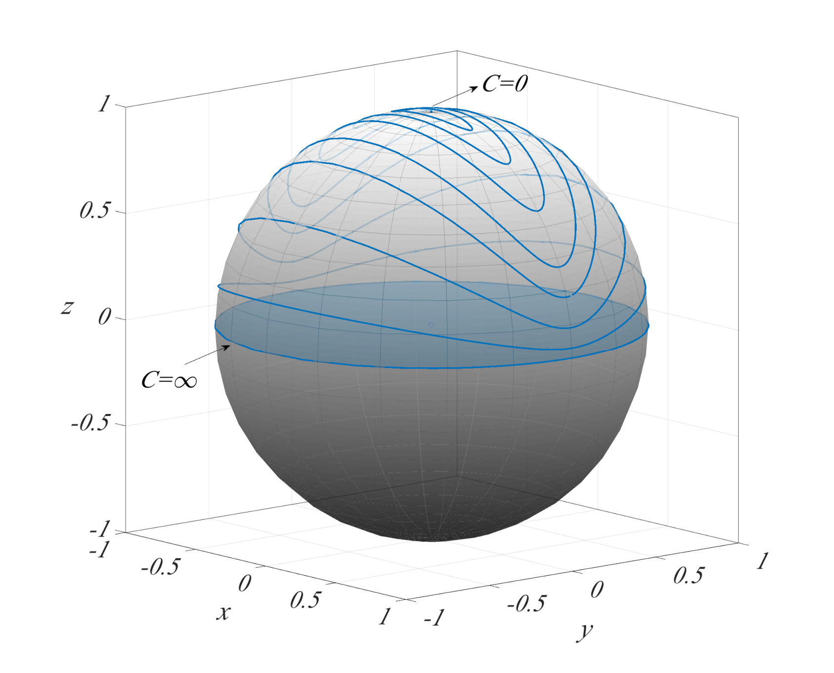
where $C$ is a constant of integration and the axis of revolution rotates in one of infinitely many possible periodic orbits depending on the value of $C$. Fig. 2 shows Jeffery orbits for different values of $C$ on a unit sphere. The Jeffery orbit on the equator of the sphere, $C\to\infty$, is called the tumbling orbit because the vector $\mathbf{p}$ tumbles in the flow-shear plane. The orbit at the pole of the sphere, $C=0$, where $\mathbf{p}$ is aligned with the vorticity direction, is called log-rolling. The period $T_{0}=2\pi(\lambda^{2}+1)/\lambda$ is constant for particles of same aspect ratio and does not depend on the initial orientation of the particle (in dimensional terms the period scales with $1/{\dot{\gamma}}_{c}$). Note that the angular velocity of the particle is not constant in time but that the particle slows down when $\mathbf{p}$ tends to the flow direction D’Avino and Maffettone 2015.

The zeroth order (Newtonian) solution of the flow field is linear, and thus we must be able to write $\dot{\boldsymbol{\gamma}}_{0}=\mathbf{M}:\mathbf{E}^{\infty}$ where $\mathbf{M}$ is a fourth order tensor that depends on the orientation of the particle alone. Substituting into (II.4) we obtain for each component of $\mathbf{\Omega}_{1}$

where repeated indices are summed. Although $\mathbf{M}$ is constructed from a known Newtonian solution the details are quite complicated (as shown in appendix ). This tensor product contains hundreds of terms and analytical evaluation of the integral proves more or less intractable and so this integral is performed numerically. After calculation of all the tensors, a trapezoidal rule in spheroidal coordinates is used for the integration with singular terms evaluated analytically.

Upon resolution of $\mathbf{\Omega}_{1}$ we calculate the periodic orbits of $\mathbf{p}$ in a shear-thinning fluid to leading order in $Cu$, namely we integrate

forward in time. An RK4 method is used for the time derivative of the particle’s orientation, and the orientation is expressed by angles $\theta$ and $\phi$ rather than vector $\mathbf{p}$ to ensure unity of its magnitude.

The dynamics of the spheroid can be divided into a rotation around the vorticity axis, $\phi$ (spinning), and rotation about the velocity axis, $\theta$ (oscillating). While the period in a Newtonian fluid, $T_{0}$, is determined only by the particle shape and shear-rate, the period in a non-Newtonian fluid, $T$, is highly dependent on initial position of the particle and $Cu$ number in shear-thinning fluids.

In Fig. 3 we show Jeffery orbits modified by shear thinning for different situations: a) different initial positions $\theta_{i}$ (for $\phi_{i}=0$), b) different initial positions on a specific Newtonian Jeffery orbit passing $(\theta_{i},\phi_{i})=(5\pi/12,0)$ c) different values of $Cu$, and finally d) different aspect ratios $\lambda$. In these results and all that follow we take values of $\beta=0.5$, and $n=0.5$. We also take $Cu=0.1$, and $\lambda=5$ unless otherwise stated. The first thing to notice in the figures is that shear-thinning rheology does not lift the degeneracy of the Jeffery orbits observed in Newtonian fluids, unlike the effects of fluid elasticity or inertia. There are still infinitely many modified ‘Jeffery’ orbits, selected by the initial condition, that repeat periodically for all time. Indeed this is somewhat expected given that the generalized Newtonian fluid constitutive equation (5), maintains the symmetries of the Stokes equations and so one should not expect a symmetry-breaking drift of the orbits in time. In general we observe that shear thinning tends to narrow the orbits in much the same way that an elongation of the particle aspect ratio does (compare Fig. 3a), c) with d). The change in a particular Newtonian Jeffery orbit due to shear thinning depends on the initial position as shown in Fig.  3b), because of course the orbits are not continuously overlapping.

As the aspect ratio of the particle increases, the particle spends a larger amount of time aligned with the flow as the torque due to the applied background flow is diminished in comparison to the hydrodynamic resistance to rotation, as dictated by (13), and thus the period of rotation increases. Much of the same thing happens with shear thinning , where the torque is reduced due to changes in the viscosity. These changes in the dynamics are illustrated in Fig. 4a) and 4b). In particular, note in Fig. 4b) that the effects of shear thinning on the particle spin ($\dot{\phi}$) are only apparent when the particle is aligned with the flow, $\phi\approx n\pi$, where shear dominates and hence the particle is slowed further due to a reduction of the viscosity. When the (slender) particle is aligned with the velocity gradient, changes in viscosity are less relevant, as the particle is essentially pushed around its orbit . Similar results were given for two-dimensional particles in Férec et al. 2018. We note that while changes in the absolute value of the the rotation rate might be small, the changes in the period of rotation can be dramatic if the angular velocity is close to zero as shown in Fig. 4c); however, while the instantaneous velocity of the particle may be accurate in either the Newtonian case, or the correction we calculate here, neglected effects such as inertia, particle eccentricity and idealizations used in Carreau model, will cumulatively affect the orbit of particle integrated over time.

As shown in Fig. 5, the effect of shear thinning varies quantitatively depending on the particular orbit but the qualitative picture is similar. In particular, the period of each orbit depends on the initial position, unlike in a Newtonian fluid, in a shear-thinning fluid each orbit has a different period.

Different orbits for different aspect ratios, $\lambda$, are shown in Fig. 6. In case of a sphere, $\lambda=1$, the period doesn’t change at all. In other words, the spherical particle is unaffected by shear thinning, as discussed in Datt and Elfring 2018. For higher aspect ratios, the orbit slows when the particle is aligned with the flow as shown in Fig. 6b), and the period $T$ thereby increases, as shown in Fig. 6c). We find that shear-thinning rheology exacerbates this effect, more substantially increasing the period for larger $\lambda$ as the shear stresses, which are needed to rotate a long slender particle aligned with the flow, are reduced by shear thinning.