Hydro+ in Action: Understanding the Out-of-Equilibrium Dynamics Near a Critical Point in the QCD Phase Diagram Preprint: MIT-CTP-5142
Abstract
Upcoming experimental programs, including the Beam Energy Scan at RHIC, will look for signatures of a possible critical point in the QCD phase diagram in fluctuation observables. To understand and predict these signatures, one must account for the fact that the dynamics of any critical fluctuations must be out-of-equilibrium: because of critical slowing down, the fluctuations cannot stay in equilibrium as the droplet of QGP produced in a collision expands and cools. Furthermore, their out-of-equilibrium dynamics must also influence the hydrodynamic evolution of the cooling droplet. The recently developed Hydro+ formalism allows for a consistent description of both the hydrodynamics and the out-of-equilibrium fluctuations, including the feedback between them. We shall provide an explicit demonstration of how this works, setting up a Hydro+ simulation in a simplified setting: a rapidity-independent fireball undergoing radial flow with an equation of state in which we imagine a critical point close to the axis of the phase diagram. Within this setup, we show that we can quantitatively capture non-equilibrium phenomena, including critical fluctuations over a range of scales and memory effects. Furthermore, we illustrate the interplay between the dynamics of the fluctuations and the hydrodynamic flow of the fireball: as the fluid cools and flows, the dynamical fluctuations lag relative to how they would evolve if they stayed in equilibrium; there is then a backreaction on the flow itself due to the out-of-equilibrium fluctuations; and, in addition, the radial flow transports fluctuations outwards by advection. Within our model, we find that the backreaction from the out-of-equilibrium fluctuations does not yield dramatically large effects in the hydrodynamic variables. Further work will be needed in order to check this quantitative conclusion in other settings but, if it persists, this will considerably simplify future modelling.
1 Introduction
Does the rapid but smooth crossover between hadron gas and quark gluon plasma (QGP) at small baryon chemical potential Aoki:2006we; Bazavov:2009zn; Borsanyi:2010cj; Bazavov:2011nk turn into a first order phase transition beyond some critical point at a nonzero ? This is one of the main unanswered questions about the phase structure of QCD matter Berges:1998rc; Halasz:1998qr; Stephanov:1998dy; Stephanov:1999zu; Rajagopal:2000wf; Stephanov:2007fk; Fukushima:2010bq; Luo:2017faz; Busza:2018rrf; Bzdak:2019pkr. To date, because of the fermion sign problem ab initio lattice calculations have proved prohibitively challenging at nonzero except via Taylor expansion in about , analytic continuation from imaginary , or via reweighting, all of which are algorithms that are based upon extracting physics at nonzero from lattice calculations whose intrinsic formulation is at . In contrast, because the ions that collide in heavy ion collisions carry nonzero net baryon number, the QGP produced in these collisions naturally inherits some nonzero – it is produced doped with baryons. At the highest collision energies accessible at the Relativistic Heavy Ion Collider (RHIC) and even more so at the Large Hadron Collider (LHC) most of the net baryon number coming from the incident nuclei ends up at high rapidity and the QGP at mid-rapidity is almost undoped. Studying the properties of QGP as a function of its doping with baryon number, which is to say mapping the phase diagram of QCD at nonzero , requires analyzing heavy ion collisions at lower collision energies where more net baryon number ends up at mid-rapidity and QGP doped to a larger is produced. This is the goal of the ongoing Beam Energy Scan (BES) program at RHIC. Data taking in the second, high statistics, phase of this program began in 2019 and is expected to conclude in 2021. The BES program provides a unique opportunity to detect signatures of the QCD critical point if such a point exists within the region of the phase diagram that is accessible to experiment. This program relies upon the Low Energy RHIC electron Cooling (LEReC) upgrade to the RHIC accelerator which will increase its luminosity at low energies as well as upgrades to the STAR detector — the Inner Time Projection Chamber (iTPC), Event Plane Detector (EPD) and Endcap Time of Flight detector (EToF). These enhancements to RHIC and STAR have been designed, in concert, to bring out fluctuation observables sensitive to the presence of a possible critical point with unprecedented high statistics for collisions with center-of-mass energies ranging between per nucleon and per nucleon, producing droplets of QGP that freezeout with MeV MeV. STAR also plans to do fixed-target collisions that will extend the reach of this program to lower center-of-mass energies, producing QGP at even larger . In addition to the BES program at RHIC, there are a number of other approved experiments anticipated in the coming years, including the Compressed Baryonic Matter (CBM) experiment at the FAIR facility at GSI, the Multi-Purpose-Detector (MPD) at the NICA accelerator in Dubna, and the CSR-External target Experiment (CEE) at the HIAF facility in China.
The anticipated experimental advances motivate a substantial theoretical effort needed to meet the challenges involved in identifying signatures of possible critical fluctuations. To maximize the discovery potential of the experimental efforts, it is crucial to understand signatures originating from the fluctuation of the critical order parameter field. In thermal equilibrium, such fluctuations grow according to universal scaling laws the closer one gets to a critical point, for example as a function of increasing , and then decrease again as the critical point is passed. In particular, therefore, we expect a nonmonotonic dependence on , and hence collision energy, in the fluctuations of the measured multiplicity of various species of hadrons Stephanov:1998dy; Stephanov:1999zu, most notably the non-Gaussian fluctuations in the multiplicity of protons Hatta:2003wn; Stephanov:2008qz; Athanasiou:2010kw; Luo:2017faz. Because also depends on rapidity, it is also of interest to analyze the rapidity dependence of these observables in collisions with a given energy Brewer:2018abr; Shen:2018pty Furthermore, the enhancement of critical fluctuation would induce universal singular behavior in the Equation of State (EoS) and in particular in transport coefficients such as bulk viscosity at and around the hypothesized critical point. See Ref. Parotto:2018pwx for the construction of a family of EoS that incorporate the expected critical behavior as well as what is known about QCD thermodynamics at lower from lattice calculations, and see Refs. Monnai:2016kud; Martinez:2019bsn for discussion of the behavior of bulk viscosity near the critical point. Since the EoS and transport coefficients control the bulk evolution of the QGP droplet produced in a heavy ion collision, signatures of a possible critical point could also manifest themselves in observables which reflect the characteristics of hydrodynamic evolution. These, too, are a focus of the BES program.
However, it has long been understood Berdnikov:1999ph that critical fluctuations cannot possibly stay in thermal equilibrium during a heavy ion collision. If there is a critical point in the equilibrium phase diagram of QCD the droplet of QGP formed in a heavy ion collision may indeed pass near it as it expands and cools. But, because the time that these rapidly cooling droplets of hot matter spend in the vicinity of the critical point is finite, and because long wavelength critical fluctuations are intrinsically slow to equilibrate, with the equilibration timescale diverging near the critical point (a phenomenon called critical slowing down), the critical fluctuations inescapably fall out-of-equilibrium. As was already apparent in the earliest work Berdnikov:1999ph and has been much further understood more recently Mukherjee:2015swa (see Ref. Yin:2018ejt for a brief review) the out-of-equilibrium fluctuations can be quite different from equilibrium expectations, certainly quantitatively and even qualitatively. Furthermore, these out-of-equilibrium fluctuations must also modify the equation of state (EoS), changing it from what it would be in equilibrium11 1 To see why this must be so, let us start by recalling that in equilibrium the correlation length of the critical fluctuations diverges and this affects the EoS, for example causing the specific heat to have a singularity. Critical slowing down means that in reality the fluctuations do not stay in equilibrium and in particular their correlation length does not diverge. This means that the specific heat should not be expected to have a singularity. This is just one example of how the out-of-equilibrium fluctuations must modify the EoS relative to what it would have been if the fluctuations were able to stay in equilibrium., and this means that they must influence the hydrodynamic evolution. The hydrodynamic evolution (expansion and cooling) drives the fluctuations away from equilibrium, and through the EoS this in turn must modify the hydrodynamic evolution.
We will adopt the newly developed Hydro+ framework to study the intertwined dynamics between the evolution of out-of-equilibrium fluctuations and the bulk hydrodynamic evolution Stephanov:2017ghc. In this approach, the dynamics of hydrodynamic variables as well as the long wavelength critical fluctuations are studied self-consistently by solving a set of coupled deterministic equations. The Hydro+ approach can describe nontrivial critical dynamics including critical slowing down, as well as modifications of the sound velocity and bulk viscosity (relative to their equilibrium values) caused by out-of-equilibrium fluctuations Stephanov:2017ghc. Via these modifications, there is a feedback on the bulk flow coming from the out-of-equilibrium critical fluctuations.
Quantitative and self-consistent modelling of the nonequilibrium evolution of critical fluctuations in heavy ion collisions is a central challenge for theoretical physicists at the present time, with the RHIC BES program now underway. This is a core goal of the Beam Energy Scan Theory collaboration, and in its full form this will require understanding of and controlled modelling of the initial stages of the collision and the freezeout dynamics as well as the coupled evolution of hydrodynamics and critical fluctuations that occurs between the early and late stages of the collision and that we shall consider. Without a treatment of the early and late stages of the collision, our study cannot by itself yield predictions to be compared to experiment. However, having the means to follow the out-of-equilibrium evolution of critical fluctuations, quantitatively, in a way that incorporates their influence on the bulk evolution as well as the influence of the bulk evolution on them is a necessary ingredient to any future effort to extract information about the presence and location of a critical point from experimental data.
The Hydro+ formalism is built upon deterministic equations for two-point functions (and, in future, higher-point functions) of the fluctuations. This is not the only possible formalism with which to achieve our goals. See Refs. Kapusta:2012zb; Kapusta:2017hfi; Sakaida:2017rtj; Nahrgang:2018afz for studies using complementary approaches based upon simulating stochastic equations. See also Refs. Akamatsu:2016llw; Murase:2016rhl; Hirano:2018diu; Singh:2018dpk for related developments in the context of fluctuating hydrodynamics away from a critical point and other studies of non-equilibrium effects around the phase transition found in Refs. Nahrgang:2011mv; Nahrgang:2011mg; Herold:2016uvv; Herold:2018ptm, which include studies of the back reaction of the order parameter fluctuations on the (stochastic) hydrodynamic variables.
The quantitative description of the future BESII data requires inputting realistic initial conditions at the relative low beam energy, solving 3d hydro+ equation at finite baryon density, and doing the appropriate freezeout of critical fluctuations. We shall not do such a study here.

Since we are not aiming for a description of BES data in this paper, what is our goal? We want to “exercise Hydro+”; we want to see Hydro+ in action. Our goal is to analyze the interplay between critical fluctuations and hydrodynamics in the simplest possible model that we can set up where the dynamical feedback between the two can be driven, with hydrodynamic expansion and cooling preventing the critical fluctuations from staying in equilibrium, and with the out-of-equilibrium fluctuations driving the bulk dynamics itself out-of-equilibrium also, and with each feeding back upon the other. There is enough complexity in this goal that in many other ways we shall make brutal simplifications. As already noted, we will (i) not attempt to discern or employ realistic initial conditions coming from the early stage dynamics of a heavy ion collision at BES energies. And, also as already noted, we will (ii) make no attempt to describe freezeout and particlization, and hence will make no predictions for experimental observables. Furthermore, instead of doing a 3+1-dimensional hydrodynamic calculation we shall (iii) assume boost-invariant longitudinal expansion and we shall (iv) assume that the expansion in the transverse directions is azimuthally symmetric. That is, we analyze radial expansion dynamics (in the presence of boost invariant longitudinal expansion) with no anisotropies. This means that we must choose initial conditions that are boost invariant and azimuthally symmetric, neither of which is a good representation of what will come from the early stages of a heavy ion collision at BES energies. The final brutal simplification that we make is that we shall (v) use an equilibrium EoS in which we place an imagined critical point near the axis of the phase diagram, as Fig. 1 illustrates. This allows us to do our entire calculation with , a considerable technical simplification. In recent years, very substantial progress has been made in relaxing all the simplifying assumptions (i)(v) in calculations done without critical fluctuations. We anticipate that in future work it will be possible to meld these advances into our own. But that is for the future.
We trust that it is apparent that our goal is not to do phenomenology. We shall provide a demonstration of how Hydro+ works in a setting in which all the physics that is unique to Hydro+ is manifest, and in an environment that is analogous to the experimentally relevant setting modulo all the simplifications. In addition to seeing how Hydro+ works we do expect that, at a qualitative level, our results can provide some guidance for what to expect from future more complete simulations. Features that we see in our results that we expect will generalize include: (a) out-of-equilibrium fluctuations lagging behind what they would be if they were able to stay in equilibrium; this qualitative feature has been expected since Ref. Berdnikov:1999ph and indeed we now see it manifest in this self-consistent setting; (b) nontrivial spatial dependence of the critical fluctuations originating because different regions of the droplet of hot fluid cool near the critical point at different times and subsequently shaped by both critical slowing down and memory effects; (c) advection of the critical fluctuations, with the radial flow in the fluid carrying them outwards; (d) imprints of the out-of-equilibrium fluctuations on the hydrodynamic variables, including the energy density and radial flow. Within our model, we find that the feedback on the hydrodynamic variables does not have dramatically large effects. Further work will be needed in order to check this quantitative conclusion in other settings but, if it persists, this will considerably simplify future modelling.
This paper is organized as follows. In Sec. 2.1, we review the ingredients of Hydro+ which are pertinent to the present study Stephanov:2017ghc, and elaborate on various subtleties and practicalities that must be faced in any explicit implementation of Hydro+ that have not been treated previously. We specify our model setup in Sections 2.2, 2.3, 2.4 and 2.5, in particular describing how we implement Fig. 1 and relate it to the Hydro+ equations in Sections 2.3 and 2.4 and describing how we initialize our calculation in Section 2.5. A reader who is only interested in results, or familiar with the Hydro+ formalism, can jump to Section 3, where we show the results of our simulations of both the out-of-equilibrium critical fluctuations and the out-of-equilibrium bulk dynamics, in the latter case looking at the deviation of the entropy density, energy density and radial flow from their equilibrium values. We conclude and look ahead in Section 4.
2 A review of Hydro+ and our model
2.1 A brief review of Hydro+
The primary goal of Hydro+ is to study the dynamics of critical fluctuations and their influence on the bulk evolution of a fluid near the critical point Stephanov:2017ghc. Specifically, we consider the Wigner transform of the equal-time two point function of the fluctuation of an order parameter field :
| (1) |
where
| (2) |
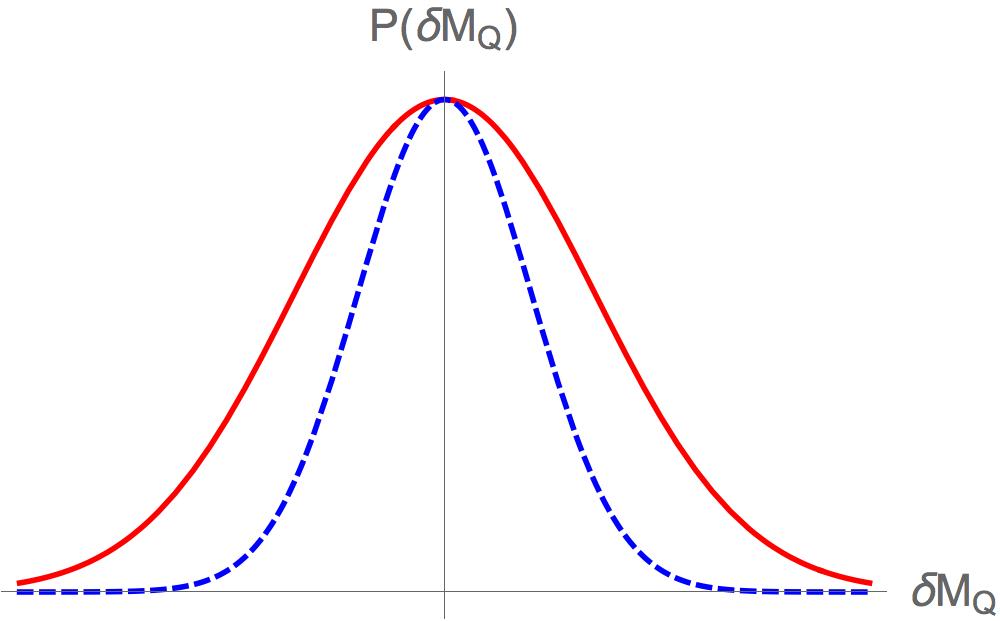
with denoting the ensemble average. describes the width of the probability distribution of at wavelength for a subsystem of a fluid labelled by coordinate at given time , see Fig. 2 for an illustration. We note that in (1) is defined in the local rest frame of the fluid. The subtlety of defining the equal-time correlator in the presence of a nontrivial flow profile was recently discussed in Ref. An:2019osr.
In Hydro+, is treated as a dynamical variable and obeys a relaxation rate equation22 2 The definition of the relaxation rate here differs from that in Ref. Stephanov:2017ghc by a factor of .:
| (3) |
In (3), we have defined33 3 According to Ref. An:2019osr, here has to be defined as the “confluent derivative”, see Ref. An:2019osr for more discussion. We will not consider this refinement here. .
| (4) |
Therefore the evolution of can be influenced by the effect of advection, as we shall illustrate through our simulation later. We will discuss the constraints on the behavior of and coming from the critical universality in Section 2.3.
The conservation laws governing the dynamics of the standard hydrodynamic variables (the energy density), (the fluid four-velocity) and (the baryon number density) take the usual form
| (5) | |||
| (6) |
where is the stress-energy tensor and is the baryon number current, each of which is related to the hydrodynamic variables via a constitutive relation. A central attribute of Hydro+ is that the out-of-equilibrium evolution of will back-react on the bulk evolution. The way that this is described in Hydro+ is that the standard constitutive relation satisfied by the stress-energy tensor is modified and becomes:
| (7) |
where we have defined:
| (8) | |||||
| (9) |
and
| (10) |
The constitutive relation (7) can be obtained from the standard hydrodynamic constitutive relation by replacing the standard pressure with and by replacing the standard shear viscosity and bulk viscosity with and , respectively. Here, the generalized pressure (see more below) depends on the hydrodynamic variables and and on the additional Hydro+ variable , with the back-reaction of the critical fluctuations on the bulk hydrodynamics being described by the dependence of these quantities on . As explained in Ref. Stephanov:2017ghc, and are in general different from their counterparts in the hydrodynamic limit, and . This is because the shear and bulk viscosity receive additional contributions originating from the slow relaxation of . These additional contributions vanish in equilibrium. Note also that the difference between and is suppressed because is a scalar function, but the difference between and is significant Stephanov:2017ghc. Since we shall be working exclusively at , we will not need the constitutive relation for , which can be found in Ref. Stephanov:2017ghc.
Remarkably, the functional dependence of on , and can all be obtained explicitly Stephanov:2017ghc, and this in turn allows for a self-consistent treatment of the back-reaction of on the hydrodynamic evolution. According to Ref. Stephanov:2017ghc, is related to the generalized entropy density by generalized thermodynamic relations, c.f. (12) below. The generalized entropy density can be expressed as , where is the ordinary entropy density and where depends on , and according to Stephanov:2017ghc:
| (11) |
where is the equilibrium value of , and where we have introduced the short-handed notation . We note that if and we also note that is negative at any . These properties are necessary since the entropy has to reach its maximum possible value when the system is in equilibrium. and are then related by the generalized thermodynamic relation Stephanov:2017ghc
| (12) |
where we have set and defined the generalized (inverse) temperature
| (13) |
with
| (14) |
The generalized pressure appearing in (7) is then given by with:
| (15) |
where the enthalpy is defined via as usual. At a formal level, this completes the specification of Hydro+. Our goal in this paper is to flesh this formalism out, turning it into equations that we shall solve, in a model context that we describe over the course of the next four subsections.
Before continuing, let us make one cautionary remark about a sense in which our notation is misleading. The quantity that we have defined describes the modification of the pressure relative to its equilibrium value that is a consequence of the deviation of away from its equilibrium value, but as we shall show in Appendix B it also describes a modification of the bulk viscosity arising from the same dynamics. The actual bulk viscosity, namely the term that multiplies in the stress-energy tensor (7) — we shall refer to it as the effective bulk viscosity — is the sum of the in and the contribution to coming from the out-of-equilibrium dynamics of that is hidden within . We illustrate this explicitly in Appendix B. Note also that in our model calculation we shall choose initial conditions with , which is maintained by the time evolution, meaning that the only source of bulk viscosity in our model calculation will be that described in Appendix B.
2.2 Our model and the Hydro+ equations we solve
Our goal in this paper is to set up a model that illustrates the nontrivial effects originating from the Hydro+ equations in a setting that at least resembles what would be needed to simulate heavy ion collisions, but to retain a level of simplicity that allows us to simplify our numerical calculations and interpret our results in such a way that we can clearly see Hydro+ in action. In the Introduction, we have described the five simplifying assumptions that we shall make in order to achieve these goals. We shall place a critical point near as in Fig. 1 and only consider the dynamics of a cooling droplet of QGP with , namely undoped QGP with zero net baryon number. This allows us to drop baryon density from the list of dynamic variables, and set the net baryon current to zero. We therefore “only” need to solve (3) and (5), which we rewrite here in a more explicit form:
| (16) |
and
| (17a) | |||||
| (17b) | |||||
| (17c) | |||||
In (17) we have introduced one more tensor made from gradients of the fluid velocity :
| (18) |
And, in (17) we have replaced and in the standard Muller-Israel-Stewart second order viscous hydrodynamic equation as considered in Ref. Baier:2006gy by and . Again following the Muller-Israel-Stewart formalism, we have introduced the shear tensor which satisfies and and obeys a relaxation equation (17c) that we shall discuss momentarily. Following Ref. Baier:2006gy, we have introduced the second order transport coefficients which is referred to as the shear relaxation time. In the limit that , we see from (17c) that which means that will approach that given by (7) (with zero bulk viscosity) and the hydrodynamic equations (17) that we use reduce to the equations of first order viscous hydrodynamics. However, as has been understood since the work of Israel and Stewart, even though we are not interested in physics to second order in gradients we must keep finite in order to ensure causality in the numerical evolution of the hydrodynamic equations. We shall use . Note that for a massless Boltzmann gas at vanishing coupling, one calculates Baier:2006um, whereas infinite-coupling calculations in SYM at large give Baier:2007ix. Treating these as respective weak- and strong-coupling estimates for , we have chosen our value to lie between these two. Note that the value of will have little effect on the dynamics; its role is to serve as a causality-preserving regulator for Müller-Israel-Stewart second-order viscous hydrodynamics.
Unfortunately, we encounter a numerical instability in our solution of (17). When we write (17c) for an azimuthally symmetric, boost-invariant system, we find two terms proportional to , and (see Eq. (6) of Ref. Baier:2006um). As in our simulation, we find that these two terms are a source of numerical noise, so we set them to zero when fm. We find that, other than fixing the instability, this procedure leaves our results unaffected.
As we explained earlier in Sec. 2.1, the difference between and is suppressed because is a scalar function. We will take
| (19) |
a reasonable value within the range motivated by comparisons between experimental measurement of, and hydrodynamic simulation of, anisotropic flow; see for example Refs. Bernhard:2016tnd; Romatschke:2017ejr. While we have set , the relaxation of still leads to an effective bulk viscosity, see (72) as discussed in Appendix. B.
As already noted in the Introduction, both to reduce computational cost and because doing so does not compromise any of our goals in this paper we consider a droplet of QGP whose longitudinal expansion is boost invariant and whose radial expansion transverse to the beam direction is azimuthally symmetric. Therefore local variables in our model will not depend on the spacetime rapidity or the azimuthal angle , but will depend on the proper time and the radial coordinate in transverse plane . We solve the Hydro+ equations numerically using a method very similar to that explained in Ref. Baier:2006gy44 4 We have developed our Hydro+ codes based on the VH1+1 hydrodynamic code which was written and made public by Paul Romatschke Baier:2006um; Baier:2006gy; Romatschke:2007jx.
In the Sections that follow, we will specify inputs needed to solve (16) and (17). To study the critical phenomenon, we wish to place a hypothetical critical point near the -axis so that critical fluctuations may grow there, i.e., and would grow around the critical temperature . We implement this in Section 2.3, where we continue the specification of our model by describing how we introduce and parameterize , which describes the critical fluctuations as they would be if they were in equilibrium, as well as the equilibration rate , both of which are needed in (16). Both depend on the equilibrium correlation length , meaning that we will need to specify our model for how depends on temperature. We complete the specification of our model in Sections 2.4 and 2.5. In Section 2.4, we introduce the EoS that we use that incorporates the presence of a critical point near as in Fig. 1, and in particular discuss how the growth of the correlation length would influence the behavior of the EoS near . In Section 2.5, we choose the initial conditions that we shall employ in our Hydro+ calculations. In each of these Sections, we shall make further simplifying assumptions, some of which we have already mentioned in the Introduction. At all stages we will recall that we are trying to achieve a setting in which we can see Hydro+ in action, watch the back-reaction between the critical fluctuations and the hydrodynamic variables that Hydro+ is designed to describe develop and ramify, and understand and assess their qualitative features. The many simplifications that we employ in order to achieve these goals mean that our results cannot be compared to data. The methods that we develop, and the insights that we gain, will become key elements of future larger simulations with fewer simplifying assumptions, and which incorporate treatments of the initial stages of the collision and of freezeout.
2.3 The parameterization of , and the correlation length
The equilibrium value of , , can be written as
| (20) |
where the susceptibility of the order parameter field in the zero momentum limit scales with as
| (21) |
with being the corresponding critical exponent55 5 The critical exponent that we denote is conventionally denoted by in literature on critical phenomena. In this paper, we use to denote the shear viscosity.. (See, for example the textbook onuki2002phase.) Here, is an equilibrium universal scaling function onuki2002phase that we can choose to have unit normalization . takes the asymptotic form onuki2002phase
| (22) |
From these universal considerations, we know the behavior of at both small and large values of :
| (23) |
Next, for simplicity we set the critical exponent to zero, since its numerical value in the 3D Ising model, onuki2002phase, is so small. That is, we simply parametrize as onuki2002phase
| (24) |
While will in general depend on temperature, we treat it as a constant because we assume that it does not vary much in the narrow band of temperatures around that are relevant to our considerations because at those temperatures is enhanced relative to its typical microscopic value, which we shall denote by and which we also take to be temperature-independent. For the same reason, we will also treat defined in (32) below as a constant.
Our results for will all be proportional to , but we shall see later that the contribution of to the Hydro+ entropy density and other thermodynamic quantities is independent of the value of . Also for simplicity, we will use the Ornstein-Zernike (OZ) form for onuki2002phase
| (25) |
which has the proper asymptotic behavior (23). Consequently, the expression that we shall use for in our calculation is
| (26) |
See Ref. Guida:1996ep for a more refined description of . In order to apply this expression in an explicit calculation, we shall need a model for how the correlation length depends on temperature.
Before turning to the correlation length itself, we must specify how the equilibration rate is related to . In general, will depend on and . When approaches its equilibrium value, so does :
| (27) |
Here will only depend on and , and near the critical point it will depend on only via the combination meaning that it can be parameterized as
| (28) |
Here, the characteristic relaxation scales as
| (29) |
with being the dynamical critical exponent. In other words, the equilibration rate for modes with will vanish as approaches infinity. This is the phenomenon of critical slowing down, and is the reason why it is impossible for critical fluctuations to stay in equilibrium arbitrarily near a critical point unless the system spends an arbitrarily long time there, which is certainly not the case in heavy ion collisions. The dynamical universal function takes the asymptotic form
| (30) |
is of order when and, in the universality class that we shall employ (see below), goes to a constant for . Therefore we find that has the following behavior:
| (31) |
For simplicity, and in the absence of any better motivated options, we shall take , which trivially satisfies (27). Next, what value shall we choose for the dynamical critical exponent and what form shall we choose for the dynamical universal scaling function appearing in in (28)? Both depend on the dynamical universality class of the critical point. The QCD critical point is in the dynamical universality class of Model H Son:2004iv; Fujii:2004za, according to the classification of Halperin and Hohenberg RevModPhys.49.435, meaning that it has .66 6 When the critical point lies out in the phase diagram of QCD at a substantial nonzero value of , its order parameter is a linear combination of the chiral condensate and . It is the fact that the order parameter incorporates a chiral condensate component that is most important to understanding the observable consequences of its fluctuations. It is the fact that it incorporates a component that is a conserved density that controls the dynamics of its fluctuations. Its equilibration is eventually determined by the diffusion of baryon density, and it is the fact that this is conserved together with the nonlinear nature of hydrodynamics which are responsible for the dynamical critical exponent taking on a value Son:2004iv. However, for a critical point close to , the critical fluctuations do not involve fluctuations in and the critical order parameter is almost purely the chiral condensate, which is not a conserved density. Since chiral symmetry is explicitly broken in QCD, the order parameter for a hypothetical critical point near may also include small components of energy and entropy density, which we shall neglect. The principal simplifications that assuming a critical point near brings us are that we need not include a mean in our hydrodynamics and that fluctuations in are not enhanced. Making this assumption also means that the critical point is to a good approximation in the dynamical universality class of Halperin and Hohenberg’s Model A and the appropriate dynamical critical exponent is Berdnikov:1999ph. So, we shall use in our calculations, and use the Model A form of RevModPhys.49.435, meaning that we take
| (32) |
Here is a constant, representing the microscopic relaxation rate away from the critical point and our choice of captures the desired asymptotics (30) and (31). (Note that the small asymptotics in (31) is that of Model A, as appropriate in our model calculation. This behavior is different in Model H, where for and for .)
As a consequence of all these considerations, the equation of motion (3) for becomes
| (33) |
where is given by (26). We will examine the dependence of our results on choices of the constant in Section 3.
To close our discussion of the equation of motion (33) for and make it fully specified, we need to parameterize the equilibrium correlation length as a function of or, as we shall choose, . Since we have placed a critical point near at some , as the droplet of plasma cools past the temperature the equilibrium correlation length will first rise will then peak at a large but finite value , and will then fall. When is much larger than the width of the critical regime, which we shall denote by , the equilibrium correlation length falls to some microscopic length ; placing the critical point near means that for a droplet that cools down the axis the equilibrium length peaks at a that is much larger than . We shall describe our choice for in an equation momentarily, but it may be helpful to look ahead to the top-left panel of Fig. 3 to see it plotted. We shall choose a simple ansatz for that approaches away from , that peaks at and, motivated by a mean theory result, that has for small if the critical point is very close to meaning that . We choose:
| (34) |
In our calculations, we shall take
| (35) |
and
| (36) |
In the top-left panel of Fig. 3, we plot as a function of , with these values of and . This expression completes our explicit specification of and the equation of motion (33) for . Our parameterization (34) of will also play into our discussion of the equation of state.
2.4 Construction of the Equation of State
In this Section, we discuss the generalized EoS, , given by (12) which, together with the inverse temperature (13) and (14), yields the expression (15). The only thing that remains in order to turn (15) into an explicit specification of is the explicit specification of the equilibrium equation of state in our model.
We shall provide by starting from a specific , and then determining via the standard thermodynamic relations
| (37) | |||||
| (38) | |||||
| (39) |
From we can also obtain the square of the sound velocity, as it is given by
| (40) |
Finally, we shall also need the standard thermodynamic relation
| (41) |
To proceed, we need an ansatz for , both the contribution associated with the critical point and the non-critical contribution. We start with the critical contribution, and begin from the textbook mean field theory result (e.g. see Ref. kardar2007statistical) that near a critical point . (By “mean field theory result” we mean that we substitute the mean field theory value for the exponent into the hyperscaling relation to obtain for spatial dimension , from which it follows that . As described in Ref. kardar2007statistical, this corresponds to including the effects of Gaussian fluctuations, as in the derivation of the Hydro+ formalism Stephanov:2017ghc.) In our calculations, we shall use the explicit form
| (42) |
and use the parameterization (34) for . The powers of come from dimensional analysis, and although we shall give an argument momentarily for our choice of the prefactor let us start by noting that we do not actually know the value of this constant of order unity. We can argue for our choice as follows. In the Ising model, the analogue of (namely the heat capacity defined upon holding the extensive thermodynamic variable fixed) is and in the mean field theory for the Ising model this is given by kardar2007statistical
| (43) |
where here and are the Ising model correlation length and its microscopic value away from the Ising model critical point. Mapping an expression like this from the Ising model onto an expression for in our model necessarily involves unknown nonuniversal factors of order unity, but there is one contribution to this factor that we can estimate: because involves two derivatives of the free energy with respect to the temperature we can expect that the prefactor that is introduced via the mapping onto our model includes a factor of , which we have set to 25, see (36). We have guessed a value of for the prefactor in the ansatz (42) because . Surely in future it will be possible to much improve on this, but we have made other more brutal simplifying assumptions elsewhere so for our purposes in this paper the ansatz (42) will suffice.
We expect that the contribution of critical fluctuations to will only become important near and that will approach that without a critical point away from . We therefore construct as follows:
| (44) |
where we shall choose to take
| (45) |
with and as in (36). The coefficients are chosen to satisfy matching conditions at the boundaries . Specifically, we will require and its first two derivatives to be continuous at . (The number of derivatives to be matched at each boundary is a matter of choice.) In order to satisfy these six constraints, we fit nonzero values of the six coefficients 77 7 With input parameters specified as we describe below, the fitted values of these parameters that we employ are given by . . In this operational way, we obtain an ansatz for the contribution to near the critical point that comes from all the degrees of freedom other than the critical order parameter. To apply this matching procedure, we first need an ansatz for that we shall use for and . We will use the following ansatz:
| (46) |
This means that in the high and low temperature limits, (and hence ) will approach temperature independent constants and , respectively. The crossover from the low temperature regime to the high temperature regime happens around with the crossover width given by . We shall choose
| (47) |
Note that can in principle be different from — there is no reason why the critical point needs to sit precisely at the midpoint of the crossover — but we use (47) for convenience. The width of the crossover in has to be larger than , and we have chosen it to be larger by a factor of three. To complete our specification of , we choose
| (48) |
with the value of for the non-interacting ideal gas QGP, namely
| (49) |
where and are the number of colors and flavors, respectively. Our choice of is motivated by the lattice QCD calculations which show that of QGP approaches from below very slowly in the high temperature limit and is around 80% of this value over a wide range of temperatures. For real QCD nuclear matter, will vanish exponentially in low temperature limit, for temperatures much below the mass of the lightest hadron. For numerical simplicity it is easier to pick a small nonzero value of as we have done, but none of the results that we shall focus on depend on this choice.


We now pause to compare the magnitude of the critical contribution to at to the non-critical contribution, as one way of checking that all the ansätze we have made look reasonable. From (42), we have , where we have used the ansatz (35), and hence for . We can compare to , as follows. corresponds to 16 bosonic degrees of freedom and 36 fermionic degrees of freedom, whereas comes from a single scalar order parameter degree of freedom whose contribution has been enhanced at by a factor of . If we take this comparison literally, it means that we have slightly underestimated , just slightly. Better to say that it gives us some confidence that the choices we have made are not unreasonable.
We now have all the ingredients we need in order to build our equation of state and all the standard thermodynamic quantities. We start from given by (44) and (42) with given by the ansatz (34) and then use (37), (38), (39) and (40) to obtain , , and the speed of sound . In Fig. 3, we plot as well as , , , , and as functions of as the red solid curves. We also show all of the thermodynamic quantities without any critical contribution as the blue dashed curves. Let us focus on which plays an important role in driving the hydrodynamic expansion. We observe as expected that vs features a minimum around since the equation of state becomes soft near a critical point. We note that also shows a maximum around . To understand this, recall the relation (c.f. (40)). has to decrease rapidly from its peak value to approach around , which in turns leads to a bump in vs .
2.5 Initial conditions
We have now specified all the elements of our model that we need in order to evolve the Hydro+ equations. All that remains in order for us to complete the full specification of our model calculation is choosing the initial conditions for the time evolution.
We shall initialize our model at
| (50) |
with an initial central temperature of 330 MeV, following Ref. Baier:2006gy. In future phenomenological modelling of BES-energy heavy ion collisions, a somewhat lower initial temperature may be appropriate. Although we know these are not realistic assumptions, we shall follow many authors including for example those of Ref. Baier:2006gy in assuming that there is no radial flow and no initially, i.e. at . We will use the standard Glauber model corresponding to a central Au-Au central collision at GeV for vs at Baier:2006gy, and use the results from Section 2.4, see e.g. Fig. 3 to initialize the -dependent values of all the other thermodynamic quantities. For simplicity, we will assume that is in equilibrium initially, i.e., . In at least one respect, this is likely unrealistic. At there will be some range of radii (at a relatively large , near the edge of the fireball) where the QGP initially has a temperature near . Our simplifying choice of initial conditions means that, for some range of , in this shell of radii we will have a large from the start. Although this is almost certainly unrealistic, since there is no reason to assume that will have had time to reach its equilibrium value in this region, it will at the same time be very helpful in exercising the Hydro+ formalism, as we will be able to watch how this feature in evolves with time. Note also that by virtue of our choice of initial conditions in our simulation will depend initially only on the magnitude of , , but not on its direction. And, as one can verify by inspecting (16), this simplification will be maintained by the time evolution.
We close this Section with a further remark about one aspect of our initial conditions that can be improved in future. Let us define and at each given through the conditions and . That is, the QGP within the shell defined by has a temperature that lies within the range . It might be tempting to view the fluid in this shell as critical, with a long correlation length, with somewhere in the shell, as if it were in equilibrium. Indeed, we have initialized as if this were so at . However, this could only make sense if , and this condition is not satisfied at very early times (c.f. Fig. 4 below). This means that a realistic initialization of within this thin shell will require an analysis of finite size effects as well as consideration of the shortness of . We leave this to future work, although we also note that we expect that the observable consequences of the critical fluctuations will be dominated by those throughout the interior of the droplet which develop later, and whose development Hydro+ is designed to describe.
3 Results
The purpose of the present work is to demonstrate the intertwined dynamics among flow and critical fluctuations . We shall present and describe results from our model calculations of the evolution of in Sec. 3.1, and then in Sec. 3.2 we shall focus on the feedback of on the bulk hydrodynamic evolution.
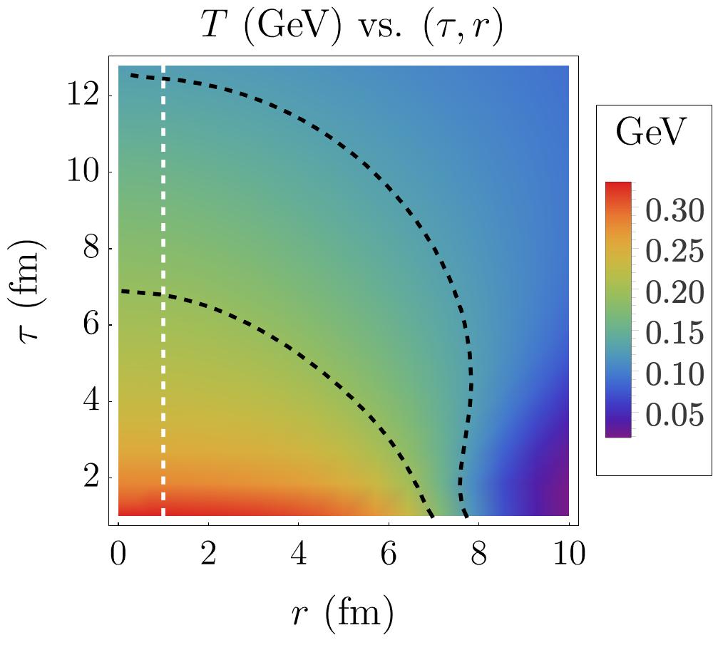
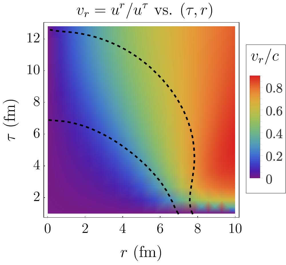
As a preamble to the presentation of our results, however, we begin in Fig. 4 by showing results for the spacetime evolution of the temperature and radial flow obtained by solving standard hydrodynamic equations using our non-critical model equation of state that we have obtained in Section 2.4 by starting from the model (46) for and applying standard thermodynamic relations. Solutions for these bulk variables obtained by using the critical EoS from Section 2.4 are similar because of the relatively small difference between the two equations of state, see Fig. 3. In Fig. 4, we observe familiar behavior of the temporal and spatial dependence of and for a fireball undergoing boost-invariant longitudinal expansion as well as radial flow. At each , the QGP fluid is hotter at smaller . As the system expands and cools, the temperature (and energy density) drops while at the same time, the radial flow starts building up due to pressure gradients. To illustrate the boundary of the critical regime where critical slowing down is expected and the use of Hydro+ is necessary we have shown the contours at which and as black dashed curves in Fig. 4.
3.1 The evolution of


We begin the presentation of the results of our model calculation of by choosing a particular value of that is representative of the interior of the fireball, , and plotting the temporal evolution of the critical fluctuations at this as a function of the momentum in the critical regime. In each of the two panels of Fig. 5, we choose four values of and plot at each , all at . We have set in this calculation. As the fireball cools, the temperature at (see the dashed white line in the left panel of Fig. 4) drops through the critical regime and the equilibrium value of , namely depicted by the dashed curves in Fig. 5, first rises as the temperature approaches from above (left panel of Fig. 5), then reaches a maximum value where passes , and finally falls as the temperature drops farther below (right panel of Fig. 5). In the left panel of Fig. 5, we see , depicted by the solid curves, rising but lagging behind , “trying to catch up”. At it catches up, because at this the equilibrium has already turned around and started coming downward. We show at , when it is at its maximum value, in both panels of Fig. 7. In the right panel of Fig. 5, we see dropping, but again lagging behind which now means that it is higher, again “trying to catch up” as drops. Note that what we have described as the solid curve lagging behind the dashed curve can equally well be described as a memory effect: the solid curve “remembers” where the dashed curve used to be, meaning that as the dashed curve rises the solid curve is below it and later when the dashed curve has dropped the solid curve “remembers” some of its former height. Regardless of the pictorial language that one chooses, the difference between the solid and dashed curves is an illustration of the out-of-equilibrium physics of the critical fluctuations that Hydro+ is designed to describe and is a direct manifestation of critical slowing down.


To complement Fig. 5, in Fig. 6 we show at at two different values of obtained from Hydro+ calculations done using four different values of . In the left panel of Fig. 6 we see that, as expected, the out-of-equilibrium effects become smaller as increases, since larger means more rapid relaxation toward equilibrium and hence the larger the value of the more rapidly the solid curve responds as the dashed curve moves, meaning the less the solid curve lags behind the rising dashed curve. In the right panel of Fig. 6, the dependence of the solid curves on the value of arises from two effects: (i) the smaller the value of the more slowly the solid curve relaxes down toward the dashed , the more the solid curve lags behind the dropping dashed curve, meaning the higher the solid curve is; (ii) for small values of the solid curve never rose as far during the earlier epoch when it was “trying to follow” the rising dashed curve, meaning that during this epoch the solid curve is lower for smaller values of . We see from the solid curves in the right panel of Fig. 6 that the first effect is dominant at larger while the second effect is more significant at the lowest values of , meaning that the solid curves with different values of can cross each other as a function of .
We can also observe, in both Figs. 5 and Fig. 6, that modes with a large enough wave vector are always close to equilibrium, for any value of and under consideration. (The value of that is “large enough” is smaller for larger values of .) In illustrating the out-of-equilibrium dynamics that Hydro+ describes, therefore, we shall henceforth focus more on smaller values of , which is to say on the longer wavelength modes.
The lagging and memory effects that we have described to this point were already present in previous studies of the evolution of critical flucuations in a spatially uniform cooling plasma Berdnikov:1999ph; Mukherjee:2015swa. Our results at the representative value of , , that we have chosen in plotting Figs. 5 and 6 share some of the same qualitative features as theirs. The two important distinctions in the present study are that: (i) we are considering a finite, inhomogeneous, fireball undergoing radial expansion and flow; and (ii) our Hydro+ treatment incorporates the feedback of the critical fluctuations on the hydrodynamic variables. We shall illustrate (i) here, and present results that bear upon (ii) in Section 3.2.


In Fig. 7, we show at two values of the wave vector , and , as functions of at three values of . We show results from Hydro+ calculations done with two values of , namely and . In all four panels, we compare with what it would have been in equilibrium, . We see that the out-of-equilibrium effects are much larger at the smaller value of and we see that the magnitude of as well as the magnitude of the out-of-equilibrium effects are much larger at the smaller value of . In the top-right panel, where and are both larger, the solid curves are close to the dashed curves at all and at all three values of . We see the largest out-of-equilibrium effects in the bottom-left panel, where and are both smaller.
We see two different effects in Fig. 7. First, we see the dynamics of lagging behind those of , remembering where it used to be. This is as we have discussed above, but now we can see the spatial dependence of these phenomena that are direct consequences of critical slowing down. The second effect is visible in all but the top-right panel of Fig. 7, but is most dramatic in the bottom-left panel in which we have chosen a smaller to focus on longer wavelength fluctuations and where we have chosen a smaller to emphasize out-of-equilibrium effects. We see in this panel that the peak in that is present in the initial conditions that we employ in the range of where the temperature of the fluid is in the critical regime when we initialize our model (recall that we assume in our model that when we initialize the dynamics at ) moves outwards at later time. This shows that the critical fluctuations can be carried outwards by advection by the outward radial flow of the bulk hydrodynamic fluid. We can only see this phenomenon, which has not been reported before, if we pick a small enough , since otherwise in this range of relaxes before there is time for it to be carried outwards. This is a particularly nice illustration of the dynamics incorporated within the equations of Hydro+, and shows that including spatial inhomogeneity as well as radial flow is not only necessary but is also interesting and important. We note, however, that the specific consequences of the advection of critical fluctuations by the flowing fluid will likely differ from those we have illustrated in our particular model study of Hydro+ in action because the specific consequence that we have shown is an artifact of our assumption that initially. Given the lumpiness of the initial conditions in realistic modelling of heavy ion collisions, however, we expect that in future Hydro+ modelling that is more realistic than ours advection will play some role, although we believe that the out-of-equilibrium effects originating from lagging behind will be more significant.
We also note that in order to control numerical artifacts (fine-scale oscillations in the solid curves) coming from the spatial lattice spacing, this lattice spacing must be small enough to render the peak in the curve smoothly. In our simulations, we have chosen a lattice spacing of fm, which makes these oscillations almost invisibly small in all the curves we have plotted. Very close inspection shows a small trace of these numerical artifacts remaining in the green and blue curves in the bottom-left panel of Fig. 7, to the left of their peaks.
We close this Section with a speculation about the value of . If there really were a critical point near the axis, as we have assumed for this model study, then for such a critical point it would be reasonable to guess that is of order 1 fm-1. For such a critical point, calculations done with would not likely be relevant. However, if there is a critical point in the QCD phase diagram it is not near . As we discussed in Section 2.3, in this case the order parameter is a linear combination of the conserved baryon number density as well as the chiral condensate, meaning that in this case rather than as in our model calculation. This suggests that if we wish to use Hydro+ calculations done within our model to gain qualitative insights into out-of-equilibrium dynamics near a possible QCD critical point we should use a value of that appears unrealistically small in our model.
3.2 Feedback of critical fluctuations on bulk evolution: qualitative discussion and quantitative results
We turn now to what can be seen as the second half of our study of Hydro+ in action. In Section 3.1 we have focused on the out-of-equilibrium dynamics of . The critical fluctuations described by are driven out of equilibrium by the time-dependence of the bulk evolution described by hydrodynamics, with the effects enhanced by critical slowing down as we have seen. The second half of the Hydro+ story is that the out-of-equilibrium critical fluctuations feedback on, and influence, the equation of state and hence the dynamics of the ordinary hydrodynamic variables that describe the bulk evolution. We turn now to illustrating these effects.

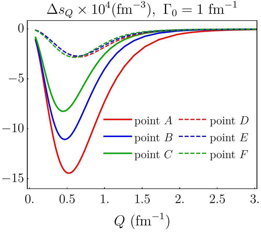
A key ingredient in the Hydro+ formulation is the generalized entropy , or its difference relative to the equilibrium entropy density . describes the modification of the entropy density due to the out-of-equilibrium critical fluctuations described by . It is given explicitly by (11). As we have discussed in Section 2.1, from we can obtain the modified equation of state, namely the modified pressure which influences the evolution of radial flow. In the left panel of Fig. 8, we plot vs . To evaluate using (11), we have taken our results for that we obtained by solving the Hydro+ equations with . We have seen in Fig. 5 that the evolution of goes out of equilibrium in two characteristic stages. First, at earlier times as rises as the cooling plasma approaches from above lags below . At later times, as drops as the plasma cools away from toward lower temperature lags above . We therefore see two bands in the left panel of Fig. 8 where is significant in magnitude. Between these bands, passes through and, at a slightly later time, crosses from below We see from the figure that is larger, meaning that out-of-equilibrium effects are larger, in the lower (hotter) of the two bands, where is approaching from above. This is because here the equilibrium is shooting upwards and can get quite far above whereas in the upper (colder) band where is chasing a falling there is less separation since never drops into negative territory. We also see from the figure that is larger at larger in the lower of the two bands. This is because the fluid at large enters the critical regime earlier in time, when the expansion rate is larger. In addition, we see the effect of the initial peak advecting outwards, which creates the bright band with positive slope in the bottom right corner of Fig. 8. Indeed, the slope of this bright band is very well approximated by the inverse of the local radial fluid velocity, , of the fluid at its location in and .
in (11) is given by an integration over all wave vectors . It is instructive to ask which range of makes the most important contribution to . To answer this question, we pick three representative points in the plane, labelled A, B and C in the left panel of Fig. 8 that lie in the lower band where is significant and three representative points labelled D, E and F that lie in the upper band, and in the right panel of Fig. 8 we plot the integrand in the expression (11) for vs. at all six of these points. Modes with a large wave vector contribute less to the integrand because these modes remain close to their equilibrium values. It is the longer wavelength modes with smaller that are driven farther out-of-equilibrium. On the other hand, the contribution of modes with small wave vectors to the integrand is suppressed just by the smaller phase space volume. So, we see that for each of the three curves in the right panel of Fig. 8 the integrand in the expression (11) is dominated by wave vectors in a range centered around in our Hydro+ calculation with . The modes in this range of wave vectors, which emerges from the dynamical calculation, make the most important contribution to the feedback of the critical fluctuations on the bulk hydrodynamic variables. This is why we have chosen as one of the two wave vectors at which we plotted in Fig. 7.
We learn an important qualitative lesson from the right panel of Fig. 8 that we have taken advantage of in our calculation, as we describe in Appendix A. The dynamical phenomena described by Hydro+ come with a natural UV cut-off in the integration of . This is the reason why need not extend our calculations to modes with arbitrarily high wave vectors in practice, and can focus on the evolution of modes that are out-of-equilibrium.


We are finally ready to look at the effects on the bulk evolution of the energy density and radial flow caused by the feedback from the out-of-equilibrium dynamics of the critical fluctuations, as described by Hydro+. From the and that we have just described we use thermodynamic relations to obtain the equation of state whose gradients drive the radial flow velocity , and in Hydro+ as in ordinary hydrodynamics this radial flow (together with the boost-invariant longitudinal expansion) determines how the droplet of plasma cools and how its energy density drops. In Fig. 9 we plot results showing how the dynamics of and in our Hydro+ calculations differ from those in our starting point, Fig. 4. Recall that in Fig. 4 we solved ordinary hydrodynamic equations, no Hydro+, and used only the non-critical equation of state from our model. We shall make comparisons between three cases:
- 1.
"B.R": solving full Hydro+, i.e. the back-reaction from the slow evolution of onto the evolution of the energy density and radial flow is taken into account.
- 2.
"no B.R.:" solving hydrodynamic equations, no Hydro+, using the critical EoS.
- 3.
"no C.P." solving hydrodynamic equations using only the non-critical EoS, as in Fig. 4.
As we have already noted in Fig. 3, the difference in the sound velocity between our critical EoS and our non-critical EoS is small, because we have assumed that peaks at 3, rather than diverging. Therefore the difference in the bulk evolution for the EoS with and without a critical point is also small. For this reason, we shall plot the differences:
| (51a) | |||
| (51b) | |||
and describe the modification of the bulk evolution due to the growth of critical fluctuations in our model as if they were in equilibrium. The black dashed curves in Fig. 9 show the fractional differences and from (51). Finally, and describe the modification of the bulk evolution in our model due to the growth of critical fluctuations as would actually occur, namely out-of-equilibrium, as described by Hydro+. The colored curves in Fig. 9 show the fractional differences and from (51).
Figure 9 showcases the relative contribution of the cases labeled “B.R.” and “no B.R.” relative to the bulk evolution with no critical point. We see that for reasonable values of the relaxation rate in the range , the effects of the back-reaction from the out-of-equilibrium critical fluctuations are greatest at and , where they amount to a difference in on top of the % difference arising solely from including the critical point in the equation of state. We have also included results with to show that at larger values of , where the critical fluctuations track more closely to their equilibrium behavior, the back-reaction on the hydrodynamic variables coming from the out-of-equilibrium fluctuations is indeed smaller.
We can understand the qualitative shapes of the back-reaction effects depicted by the colored curves in Fig. 9 relative to the black dashed “no B.R.” curves. The largest contribution to the back-reaction on the hydrodynamic variables arises from the modification to the pressure gradient , which is given by first and second derivatives of , see (15). Since pressure gradients drive the radial flow, this translates directly into a modification of . Modifications of yield modifications of the energy density since is diluted more rapidly in places where is greater. Looking at a fixed slice of Fig. 8, we see that at some fixed the quantity should have two positive peaks, meaning that its second derivative should change signs four times. The distortions in the colored “no B.R.” energy density curves indeed changes sign four times. This is most easily visible in the middle panels at fm where we can see that (as a function of increasing ) the energy density is first below the no-back-reaction black dashed curve, then above, then below, then above and finally below again. This is the case also in the upper panels; in the lower panels, the last sign change occurs at larger values of than we have plotted. We also note that whenever the radial velocity distortion is negative, the energy distortion is positive, reflecting the fact that when a portion of the fluid expands relatively slower, it cools less, so its energy density decreases less. For example, the largest distortion in that we see, the downward-going spike at just below 7 fm at fm, corresponds directly to the largest distortion in which is indeed an upward-going spike.
We close by noting that all the effects of the back-reaction of the out-of-equilibrium critical fluctuations on the hydrodynamic variables that we have illustrated in Fig. 9 are sufficiently small that in future more realistic modelling of heavy ion collisions it may suffice for phenomenological purposes to use Hydro+ to describe the growth and out-of-equilibrium dynamics of while neglecting the back-reaction of the critical fluctuations on the hydrodynamic variables and the bulk evolution.
4 Discussion and Outlook
We have successfully exercised the newly developed Hydro+ formalism, testing all of its elements in a concrete model setting where we have been able to see all aspects of the formalism in action. The model that we have used is simplified in a number of ways, meaning that results from this study itself cannot be used to compare to experimental measurements in heavy ion collisions, for example from the Beam Energy Scan program at RHIC. This means that there are opportunities for future extensions of this work, as we discuss below. First, though, some remarks about our results are in order, as at a qualitative level they should provide some guidance as to what phenomena to expect in heavy ion collisions that cool near a critical point in the QCD phase diagram and they should certainly provide qualitative guidance for future quantitative calculations of hydrodynamic evolution near a critical point.
Hydro+ allows us to evolve bulk hydrodynamic variables that describe the expansion and cooling of a droplet of QGP together with critical fluctuations that are necessarily out-of-equilibrium in a self-consistent fashion, including the feedback of each upon the other. In our model we have seen this interplay manifest explicitly.
As the droplet in our model cools and approaches near a critical point, we see the magnitude of the critical fluctuations grow, but lag behind how they would have grown if they were in equilibrium. As the critical point is passed and the droplet cools further, the critical fluctuations decrease in magnitude, but here again they lag – staying larger than they would have if they were in equilibrium. This lag is the central reason why out-of-equilibrium physics is important near a critical point, as has long been realized from more simplified treatments. What we have been able to do for the first time is to watch all of this physics as a function of position in a spatially inhomogeneous model. We have also seen that the fact that the droplet expands radially introduces a further phenomenon: once critical fluctuations have been sourced, they are advected by the flowing fluid, carried outwards to larger radii than where they were born.
A considerable fraction of the technical challenge in implementing Hydro+ comes from calculating the back-reaction that the out-of-equilibrium critical fluctuations exert on the hydrodynamic variables. We have completed this computation explicitly, calculating the back-reaction on the entropy density, pressure, energy density, speed of sound and radial velocity, and plotting the changes induced in the entropy and energy density as well as in the radial velocity. We find that the back-reaction effects are small, in a few cases larger than 1% but often smaller than that. As the model is improved (see below) this should be rechecked but this gives us hope that in future phenenological modelling of heavy ion collisions at BES energies it may suffice to use only the “first half” of Hydro+, namely the calculation of the evolution of critical fluctuations in a dynamical hydrodynamic background, without including the “second half”, namely the calculation of the back-reaction on the hydrodynamics. Note also that, as we explained in Section 2.4, while the critical fluctuations from a single order parameter degree of freedom are enhanced near a critical point, the thermodynamics of the bulk comes from a strongly coupled liquid built from 16 bosonic degrees of freedom and 36 fermionic degrees of freedom. Therefore the influence of critical fluctuations on the entropy density is small if the fluctuations are in equilibrium, as we saw in Fig. 3, and the effects of the back-reaction from the out-of-equilibrium fluctuations on the entropy density which are also small can become comparable in magnitude. The smallness of the effects of the fluctuations on the thermodynamic variables indicates that the observables that will be important in the experimental search for a possible critical point are those sensitive to the direct effects of the fluctuations themselves, rather than modifications to flow observables.
We close by listing some of the many ways in which our simplified model can be extended.
- •
Developing Hydro+ calculations for hydrodynamic backgrounds whose expansion is not boost invariant and not azimuthally symmetric.
- •
Developing Hydro+ calculations in which the critical point is far from , built upon an equilibrium equation of state like that in Ref. Parotto:2018pwx rather than the simplified one that we have employed. Working at nonzero introduces the physics of baryon number diffusion, which will lag due to the enhancement in the baryon susceptibility. It may also enhance some of the effects that we have seen due to the fact that in this case the order parameter includes a conserved component the relaxation time will be somewhat longer than in our calculation. For this reason, the back-reaction of the fluctuations on the hydrodynamics should be analyzed as we have done, but if it is as small as we have found it may suffice to neglect the back-reaction in phenomenological modelling, making it possible to rely upon hydrodynamic modelling as is already being developed in Refs. Denicol:2018wdp; Du:2019obx, together with a Hydro+ analysis of the critical fluctuations without back-reaction.
- •
Quantitative calculations of how the Hydro+ fields, including which describes the magnitude of critical fluctuations (for example in in the mass of the proton) particlize and freeze out are a necessity before phenomenological modelling of experimental observables that are sensitive to the fluctuations can begin.
- •
Much work remains to be done in order to model the initial conditions for Hydro+. Much work is already underway on modelling the initial conditions for hydrodynamics Shen:2017bsr, and one can envision future calculations in which standard (non-critical) event-by-event fluctuations in the initial conditions for the energy density and hydrodynamic flow are implemented in an event-by-event Hydro+ calculation. In addition, our assumption that begins in equilibrium must be revisited. This is perhaps a reasonable assumption deep within the fireball, where the initial temperatures are hot and initializing in equilibrium means initializing it at a small value and watching it grow as the QGP cools, as we have done. Our strict assumption of initial equilibrium for everywhere, though, means that we have initialized it with a large magnitude in an outer shell of radii where the temperatures are near the critical point initially. This is unrealistic and needs to be handled in a more sophisticated fashion in future phenomenological modelling.
Opportunities abound; we look forward to seeing Hydro+ in action in more and more realistic model settings in anticipation of the day when predictions from a simulation framework for BES collisions that incorporates a Hydro+ analysis of critical fluctuations can be compared to experimental data, with the goal of first finding a critical point in the QCD phase diagram or excluding its presence in the regime explored in BES energy collisions and second, if one is found, using the comparison between theory and experiment to learn about the out-of-equilibrium dynamics around it.
Acknowledgements.
We are grateful to Marcus Bluhm, Lipei Du, Ulrich Heinz, Iurii Karpenko, Volker Koch, Marlene Nahrgang, Paul Romatschke, Thomas Schäfer, Chun Shen and Misha Stephanov for helpful conversations. KR gratefully acknowledges the hospitality of the CERN Theory group. GR is supported by a National Science Foundation Graduate Research Fellowship. This work was supported by the U.S. Department of Energy, Office of Science, Office of Nuclear Physics, within the framework of the Beam Energy Scan Theory (BEST) Topical Collaboration and grant DE-SC0011090.Appendix A Some details regarding numerical implementation
It is convenient to regroup quantities into dimensionless combinations for numerical implementation. We measure wavectors in units of
| (52) |
According to (20),(24) and (25), we have
| (53) |
Since only depends on
| (54) |
which is dimensionless, we do our numerical calculations in terms of rescaled and such that
| (55) |
where for later convenience, we have defined a dimensionless quantity
| (56) |
We next rewrite our expression (14) for and (15) for as
| (57) |
and
| (58) | |||||
Likewise, we can write in terms of and , obtaining
| (59) | |||||
Continuing, we define as:
| (60a) | |||||
| (60b) | |||||
And, since
| (61a) | |||||
| (61b) | |||||
we have
| (62a) | |||||
| (62b) | |||||
Here, we will use the expression (25) for the function :
| (63) |
Therefore and in (61) only depend on , We finally have:
| (64a) | |||||
| (64b) | |||||
We use (64a) and (64b) in our numerical implementation of Hydro+, with the expressions for and given by (61).
In our numerical implementation of Hydro+, in order to evaluate the integrals over wave vector we must discretize and we can only keep a finite number of values of . Fortunately, as illustrated in the right panel of Fig. 8 and discussed in the text there, Hydro+ comes with a natural UV cut-off. Very high modes do not contribute much to the Hydro+ integrals that we wish to evaluate because these modes stay close to equilibrium. So, we will perform integrals over by selecting finitely many values , for example writing (11) as
| (65) |
where is the volume element for the ’th mode, whose wave vector is . Due to radial symmetry, we need only specify the magnitude of our wave vectors. Therefore, the volume element satisfies , accounting for the fact that all modes with wave vectors within a shell of thickness and radius contribute to the above integral equally. As we have noted, we choose to discretize unevenly in wave vector. In fact, what we have found convenient is to divide the -integral into three ranges, over each of which we discretize evenly in inverse-wave-vector, which is to say evenly in wavelength, but to choose the spacing between the wavelengths of the modes differently in three ranges. We do so motivated by the right panel of Fig. 8, which tells us that we can choose a coarse spacing of ’s for both the shortest and longest wavelength modes, since neither regime contributes significantly, while choosing a finer spacing of ’s in the regime of wave vectors whose contribution to the integral is most significant. Specifically, in our calculation we use modes with of them coarsely spaced at large and of them coarsely spaced at small and the rest more finely spaced in between, as follows:
| (66) |
where we set fm, and fm, meaning that we have 10 UV modes above fm-1 and 10 IR modes below fm -1, and 100 modes between fm-1 and fm-1. Finally, is the maximum radius of our box, and is 12.5 fm in this paper. (We have doubled the box size to check convergence.) Finally, we define for and .
Appendix B Feedback from on and
In this Appendix, we will provide a qualitative illustration of how effects originating from deviations between and its equilibrium value modify the bulk viscosity and sound velocity, in so doing extending the previous analysis of Ref. Stephanov:2017ghc. Our analytical discussion in this Appendix is intended only as illustrative; all of these out-of-equilibrium effect are taken into account via the full, numerical, Hydro+ calculation of .
In order to pursue this illustration analytically as far as possible, we shall only treat the case where is close to its equilibrium value. That is, recalling the definition (54), we shall consider the limit . By construction, vanishes when is in equilibrium.
We will first assess the contribution to the bulk viscosity in the limit (54) by studying how would react in response to expansion of the medium. We recast the equation of motion (16) for into an equation of motion for and keep only terms that are linear in , obtaining
| (67) |
where we have introduced the abbreviated notation
| (68) |
In addition, we have replaced with in (16), as we did in Section 2.
Since the equilibration rate is an increasing function of , modes with a high enough momentum will always be able to “catch up” with the changing value of the equilibrium as the medium expands, meaning that their values of can be estimated by finding the which makes the RHS of (67) vanish:
| (69) |
where we have used the hydrodynamic equation , and where we have replaced with , which is adequate for the desired accuracy of the present analysis. The expression (69) implies that although as (as happens as ) and tends to zero as these high momentum modes attain their equilibrium values, we see that for large but not infinite the leading correction to is proportional to .
To confirm that the out-of-equilibrium contribution (69) to in turn yields a contribution to that multiplies and hence is in fact a contribution to the bulk viscosity, we substitute (69) into (11), (14) and (15) and obtain:
| (70) |
where we have only kept terms up to linear order in and where we have introduced a lower limit in the integral arising in (70) since (69) is only valid for high momentum modes which are near equilibrium. We note in passing that the dominant contribution in (70) arises from in the numerator of (15). We finally substitute (70) into the constitutive relation (7), and obtain the contribution to the stress-energy tensor driven by the expansion of the medium:
| (71) |
with
| (72) |
where the first term is the contribution originating from the out-of-equilibrium dynamics of that we have estimated in this Appendix. It is evident from (72) that this dynamics induces an effective bulk viscosity even if is zero.
It is worth noting that in the long time limit, or in the limit in which the expansion is so slow that modes at all satisfy (69), and we then have from (72):
| (73) |
The expression (73) describes the contribution from to the bulk viscosity close to equilibrium; this expression has been obtained previously by diagrammatic calculations based on mode-mode coupling theory onuki2002phase or by solving the linearized Hydro+ equations Stephanov:2017ghc.
We also note that since near the critical point, which is the phenomenon of critical slowing down, the expression (73) is only valid near a critical point for very slow expansion. That said, we observe that (73) indicates that when the contribution becomes singular. It is this observation that motivates us to simplify our model calculation by choosing , meaning that the only contributions to the bulk viscosity are those that come from the out-of-equilibrium dynamics of through its contribution to . In any realistic context, because of critical slowing down. Consequently, the ratio
| (74) |
can be of the order unity.
We turn now to looking at how the out-of-equilibrium dynamics of the low momentum modes of contribute to , and through serve to modify the sound velocity. In the remainder of this Appendix, we provide an illustration of this effect.
Let us express in terms of and using (58) and , and take the limit :
| (75) |
To derive (75), we also made the replacement and in (58). We see from the expression (75) that through its contribution to the out-of-equilibrium dynamics of contributes to the square of the sound velocity, , which we shall denote by to distinguish it from the equilibrium . From (75), we have
| (76) | |||||
We have introduced an upper bound in the integration, , in order to focus on far-from-equilibrium modes, and used (62a) to obtain the second line of (76). Note that is the universal scaling function introduced in (20). In the third line of (76), we used the approximation
| (77) |
to simplify the expression. Note that (77) is consistent with our parameterization (34) of , which satisfies around . Note also that (76) is positive definite, meaning that the out-of-equilibrium is larger than , which is to say the out-of-equilibrium pressure is stiffer than the equilibrium .
In order to get a qualitative sense of the importance of the out-of-equilibrium correction to the equation of state, we close this Appendix by comparing in (76) to the difference between the equilibrium for our non-critical equation of state and our critical equation of state:
| (78) |
where we have used the fact , see Sec. 2.4. Since is one of the important parameters that controls the hydrodynamical evolution, this comparison provides qualitative guidance as to whether () is comparable with () (cf. (51)). In particular, if is of the same order as , we also expect () and () to be similar in magnitude.
The explicit ansatz for that we employ in our model is given by (42); we reproduce it here for convenience 88 8 In (42), has been replaced by , the value we have used in our model calculation.:
| (79) |
where (c.f. Ref. kardar2007statistical)
| (80) |
where here and are Ising model quantities. We have used
| (81) |
to evaluate the integration over . Substituting (80) and (79) into (78), we have
| (82) |
Taking the ratio between in (82) with in (76), we finally have:
| (83) |
We note the integration over in (82) will be saturated when . Therefore the ratio in (83) will be of order unity if , a result that seems quite natural indeed.
References
- (1) Y. Aoki, G. Endrodi, Z. Fodor, S. D. Katz and K. K. Szabo, The Order of the quantum chromodynamics transition predicted by the standard model of particle physics, Nature 443 (2006) 675 [hep-lat/0611014].
- (2) A. Bazavov et al., Equation of state and QCD transition at finite temperature, Phys. Rev. D80 (2009) 014504 [0903.4379].
- (3) S. Borsanyi, G. Endrodi, Z. Fodor, A. Jakovac, S. D. Katz, S. Krieg et al., The QCD equation of state with dynamical quarks, JHEP 11 (2010) 077 [1007.2580].
- (4) A. Bazavov et al., The chiral and deconfinement aspects of the QCD transition, Phys. Rev. D85 (2012) 054503 [1111.1710].
- (5) J. Berges and K. Rajagopal, Color superconductivity and chiral symmetry restoration at nonzero baryon density and temperature, Nucl. Phys. B538 (1999) 215 [hep-ph/9804233].
- (6) A. M. Halasz, A. D. Jackson, R. E. Shrock, M. A. Stephanov and J. J. M. Verbaarschot, On the phase diagram of QCD, Phys. Rev. D58 (1998) 096007 [hep-ph/9804290].
- (7) M. A. Stephanov, K. Rajagopal and E. V. Shuryak, Signatures of the tricritical point in QCD, Phys. Rev. Lett. 81 (1998) 4816 [hep-ph/9806219].
- (8) M. A. Stephanov, K. Rajagopal and E. V. Shuryak, Event-by-event fluctuations in heavy ion collisions and the QCD critical point, Phys. Rev. D60 (1999) 114028 [hep-ph/9903292].
- (9) K. Rajagopal and F. Wilczek, The Condensed matter physics of QCD, in At the frontier of particle physics. Handbook of QCD. Vol. 1-3, M. Shifman and B. Ioffe, eds., pp. 2061–2151, (2000), hep-ph/0011333, DOI.
- (10) M. Stephanov, QCD phase diagram: An Overview, PoS LAT2006 (2006) 024 [hep-lat/0701002].
- (11) K. Fukushima and T. Hatsuda, The phase diagram of dense QCD, Rept. Prog. Phys. 74 (2011) 014001 [1005.4814].
- (12) X. Luo and N. Xu, Search for the QCD Critical Point with Fluctuations of Conserved Quantities in Relativistic Heavy-Ion Collisions at RHIC : An Overview, Nucl. Sci. Tech. 28 (2017) 112 [1701.02105].
- (13) W. Busza, K. Rajagopal and W. van der Schee, Heavy Ion Collisions: The Big Picture, and the Big Questions, Ann. Rev. Nucl. Part. Sci. 68 (2018) 339 [1802.04801].
- (14) A. Bzdak, S. Esumi, V. Koch, J. Liao, M. Stephanov and N. Xu, Mapping the Phases of Quantum Chromodynamics with Beam Energy Scan, 1906.00936.
- (15) Y. Hatta and M. A. Stephanov, Proton number fluctuation as a signal of the QCD critical endpoint, Phys. Rev. Lett. 91 (2003) 102003 [hep-ph/0302002].
- (16) M. A. Stephanov, Non-Gaussian fluctuations near the QCD critical point, Phys. Rev. Lett. 102 (2009) 032301 [0809.3450].
- (17) C. Athanasiou, K. Rajagopal and M. Stephanov, Using Higher Moments of Fluctuations and their Ratios in the Search for the QCD Critical Point, Phys.Rev. D82 (2010) 074008 [1006.4636].
- (18) J. Brewer, S. Mukherjee, K. Rajagopal and Y. Yin, Searching for the QCD critical point via the rapidity dependence of cumulants, Phys. Rev. C98 (2018) 061901 [1804.10215].
- (19) C. Shen and B. Schenke, Dynamical initialization and hydrodynamic modeling of relativistic heavy-ion collisions, Nucl. Phys. A982 (2019) 411 [1807.05141].
- (20) P. Parotto, M. Bluhm, D. Mroczek, M. Nahrgang, J. Noronha-Hostler, K. Rajagopal, C. Ratti, T. Schäfer, and M. Stephanov, Lattice-QCD-based equation of state with a critical point, 1805.05249.
- (21) A. Monnai, S. Mukherjee and Y. Yin, Phenomenological Consequences of Enhanced Bulk Viscosity Near the QCD Critical Point, Phys. Rev. C95 (2017) 034902 [1606.00771].
- (22) Martinez, M. and Schäfer, T. and Skokov, V., Critical behavior of the bulk viscosity in QCD, 1906.11306.
- (23) B. Berdnikov and K. Rajagopal, Slowing out-of-equilibrium near the QCD critical point, Phys.Rev. D61 (2000) 105017 [hep-ph/9912274].
- (24) S. Mukherjee, R. Venugopalan and Y. Yin, Real time evolution of non-Gaussian cumulants in the QCD critical regime, Phys. Rev. C92 (2015) 034912 [1506.00645].
- (25) Y. Yin, The QCD critical point hunt: emergent new ideas and new dynamics, 1811.06519.
- (26) M. Stephanov and Y. Yin, Hydrodynamics with parametric slowing down and fluctuations near the critical point, Phys. Rev. D98 (2018) 036006 [1712.10305].
- (27) J. I. Kapusta and J. M. Torres-Rincon, Thermal Conductivity and Chiral Critical Point in Heavy Ion Collisions, Phys. Rev. C86 (2012) 054911 [1209.0675].
- (28) J. I. Kapusta and C. Plumberg, Causal Electric Charge Diffusion and Balance Functions in Relativistic Heavy Ion Collisions, Phys. Rev. C97 (2018) 014906 [1710.03329].
- (29) M. Sakaida, M. Asakawa, H. Fujii and M. Kitazawa, Dynamical evolution of critical fluctuations and its observation in heavy ion collisions, Phys. Rev. C95 (2017) 064905 [1703.08008].
- (30) Nahrgang, Marlene and Bluhm, Marcus and Schäfer, Thomas and Bass, Steffen A., Diffusive dynamics of critical fluctuations near the QCD critical point, Phys. Rev. D99 (2019) 116015 [1804.05728].
- (31) Y. Akamatsu, A. Mazeliauskas and D. Teaney, A kinetic regime of hydrodynamic fluctuations and long time tails for a Bjorken expansion, Phys. Rev. C95 (2017) 014909 [1606.07742].
- (32) K. Murase and T. Hirano, Hydrodynamic fluctuations and dissipation in an integrated dynamical model, Nucl. Phys. A956 (2016) 276 [1601.02260].
- (33) T. Hirano, R. Kurita and K. Murase, Hydrodynamic fluctuations of entropy in one-dimensionally expanding system, Nucl. Phys. A984 (2019) 44 [1809.04773].
- (34) M. Singh, C. Shen, S. McDonald, S. Jeon and C. Gale, Hydrodynamic Fluctuations in Relativistic Heavy-Ion Collisions, Nucl. Phys. A982 (2019) 319 [1807.05451].
- (35) M. Nahrgang, S. Leupold and M. Bleicher, Equilibration and relaxation times at the chiral phase transition including reheating, Phys. Lett. B711 (2012) 109 [1105.1396].
- (36) M. Nahrgang, S. Leupold, C. Herold and M. Bleicher, Nonequilibrium chiral fluid dynamics including dissipation and noise, Phys. Rev. C84 (2011) 024912 [1105.0622].
- (37) C. Herold, M. Nahrgang, Y. Yan and C. Kobdaj, Dynamical net-proton fluctuations near a QCD critical point, Phys. Rev. C93 (2016) 021902 [1601.04839].
- (38) C. Herold, A. Kittiratpattana, C. Kobdaj, A. Limphirat, Y. Yan, M. Nahrgang et al., Entropy production and reheating at the chiral phase transition, Phys. Lett. B790 (2019) 557 [1810.02504].
- (39) X. An, G. Basar, M. Stephanov and H.-U. Yee, Relativistic Hydrodynamic Fluctuations, 1902.09517.
- (40) M. Stephanov, On the sign of kurtosis near the QCD critical point, Phys.Rev.Lett. 107 (2011) 052301 [1104.1627].
- (41) R. Baier and P. Romatschke, Causal viscous hydrodynamics for central heavy-ion collisions, Eur. Phys. J. C51 (2007) 677 [nucl-th/0610108].
- (42) R. Baier, P. Romatschke and U. A. Wiedemann, Dissipative hydrodynamics and heavy ion collisions, Phys. Rev. C73 (2006) 064903 [hep-ph/0602249].
- (43) R. Baier, P. Romatschke, D. T. Son, A. O. Starinets and M. A. Stephanov, Relativistic viscous hydrodynamics, conformal invariance, and holography, JHEP 04 (2008) 100 [0712.2451].
- (44) J. E. Bernhard, J. S. Moreland, S. A. Bass, J. Liu and U. Heinz, Applying Bayesian parameter estimation to relativistic heavy-ion collisions: simultaneous characterization of the initial state and quark-gluon plasma medium, Phys. Rev. C94 (2016) 024907 [1605.03954].
- (45) P. Romatschke and U. Romatschke, Relativistic Fluid Dynamics In and Out of Equilibrium, Cambridge Monographs on Mathematical Physics. Cambridge University Press, 2019, 10.1017/9781108651998, [1712.05815].
- (46) P. Romatschke, Causal viscous hydrodynamics for central heavy-ion collisions. II. Meson spectra and HBT radii, Eur. Phys. J. C52 (2007) 203 [nucl-th/0701032].
- (47) A. Onuki, Phase Transition Dynamics. Cambridge University Press, 2002.
- (48) R. Guida and J. Zinn-Justin, 3-D Ising model: The Scaling equation of state, Nucl. Phys. B489 (1997) 626 [hep-th/9610223].
- (49) D. Son and M. Stephanov, Dynamic universality class of the QCD critical point, Phys.Rev. D70 (2004) 056001 [hep-ph/0401052].
- (50) H. Fujii and M. Ohtani, Soft modes at the critical end point in the chiral effective models, Prog. Theor. Phys. Suppl. 153 (2004) 157 [hep-ph/0401028].
- (51) P. C. Hohenberg and B. I. Halperin, Theory of dynamic critical phenomena, Rev. Mod. Phys. 49 (1977) 435.
- (52) M. Kardar, Statistical Physics of Particles. Cambridge University Press, 2007.
- (53) G. S. Denicol, C. Gale, S. Jeon, A. Monnai, B. Schenke and C. Shen, Net baryon diffusion in fluid dynamic simulations of relativistic heavy-ion collisions, Phys. Rev. C98 (2018) 034916 [1804.10557].
- (54) L. Du and U. Heinz, (3+1)-dimensional dissipative relativistic fluid dynamics at non-zero net baryon density, 1906.11181.
- (55) C. Shen and B. Schenke, Dynamical initial state model for relativistic heavy-ion collisions, Phys. Rev. C97 (2018) 024907 [1710.00881].