Electronic structure of 30° twisted double bilayer graphene
Abstract
In this paper, the electronic properties of 30° twisted double bilayer graphene, which loses the translational symmetry due to the incommensurate twist angle, are studied by means of the tight-binding approximation. We demonstrate the interlayer decoupling in the low-energy region from various electronic properties, such as the density of states, effective band structure, optical conductivity and Landau level spectrum. However, at points, the interlayer coupling results in the appearance of new Van Hove singularities in the density of states, new peaks in the optical conductivity and importantly the 12-fold-symmetry-like electronic states. The k-space tight-binding method is adopted to explain this phenomenon. The electronic states at points show the charge distribution patterns more complex than the 30° twisted bilayer graphene due to the symmetry decrease. These phenomena appear also in the 30° twisted interface between graphene monolayer and AB stacked bilayer.
I Introduction
In theory, a twisted bilayer graphene (TBG) can transform from a crystalline (commensurate configuration) to quasi-crystalline (incommensurate configuration) depending on the twist angleShallcross et al. 2010. At the large twist angle (15°), the TBG has electronic properties very similar to those of two decoupled graphene monolayers.Berger et al. 2006; Hass et al. 2008; Miller et al. 2009; Sadowski et al. 2006; Sprinkle et al. 2009; de Heer et al. 2010; Sprinkle et al. 2010; van Wijk et al. 2015 The Fermi velocity can be reduced by decreasing the twist angle.Suárez Morell et al. 2010a; Yin et al. 2015 At the so-called magic angle ( 1.1°), the Fermi velocity becomes zero and the flat bands appear in the vicinity of the Fermi levelSuárez Morell et al. 2010b; Bistritzer and MacDonald 2011. Accordingly, the TBG at the small twist angle as a model system of strongly correlated electrons has drawn much attention due to the novel electronic properties, such as the unconventional superconductivityCao et al. 2018a; Po et al. 2018; Yankowitz et al. 2019 and correlated insulator phasesCao et al. 2018b.
The 30° TBG, an incommensurate bilayer configuration, has been grown successfully on H-SiC(0001)Ahn et al. 2018, Pt(111)Yao et al. 2018, Cu-Ni(111)Takesaki et al. 2016 and CuPezzini et al. 0; Deng et al. 2020a surfaces. As the first two dimensional quasicrystal based on graphene, 30° TBG has received increasing attention both experimentally and theoreticallyLin et al. 2018; Park et al. 2019; Koren and Duerig 2016; Suzuki et al. 2019; Moon et al. 2019; Yan et al. 2019a; Yu et al. 2019. A method to grow high-quality 30° TBG epitaxially on SiC using borazine as a surfactant has also been proposedLin et al. 2018. The 12-fold rotation symmetry and quasi-periodicity of 30° TBG have been demonstrated by various measurements, such as the Raman spectroscopy, low-energy electron microscopy/diffraction (LEEM/LEED), transmission electron microscopy (TEM) and scanning tunneling microscopy (STM) measurements.Yao et al. 2018; Ahn et al. 2018; Takesaki et al. 2016; Yan et al. 2019b; Lin et al. 2018 A number of Dirac cones, especially the mirror-symmetric ones, have been observed by the angle resolved photoemission spectroscopy (ARPES) measurementsAhn et al. 2018; Yao et al. 2018. The quasicrystalline order in 30° TBG can induce unique localization of electrons without any extrinsic disordersPark et al. 2019; Moon et al. 2019. All these peculiar properties, especially the quasi-periodicity, make 30° TBG much different from graphene monolayer, although it has electronic properties very similar to those of two decoupled graphene monolayers in the vicinity of the Fermi level.Deng et al. 2020b
Recently, the twisted double bilayer graphene (TDBG) consisting of two -stacked bilayers, has received much attention especially on the propertiesLiu et al. 2019; Cao et al. 2019; Scheurer et al. 2019; Shen et al. 2020; Burg et al. 2019 associated with the strongly correlated electrons in the electrically tunable flat bandHaddadi et al. 2020; Chebrolu et al. 2019; Choi and Choi 2019; Koshino 2019, such as the superconductivity, magnetic phase transition and correlated insulating state. Besides, the TDBG under the electric field was found to be a valley Hall insulator.Koshino 2019 A generic twisted multilayer graphene, layers on top of layers with a twist angle, possesses two topologically nontrivial flat bands, which exhibit a Chern-number hierarchy.Liu et al. 2019 Similar to the 30° TBG, the 30° TDBG is expected to possess some striking properties due to the disappearance of the translational symmetry. More importantly, the successful fabrication of 30° TBG and accurate determination of some key structural parameters (such as twist angle, stacking order and interlayer spacing) in experimentBrown et al. 2012; Wu et al. 2016 ensure the realization of 30° TDBG in the near future. Therefore, in this paper, we study the effect of the 30° twisted interface between two AB stacked graphene bilayers. The 30° twisted interface between graphene monolayer and AB stacked bilayer is also discussed.
II methods
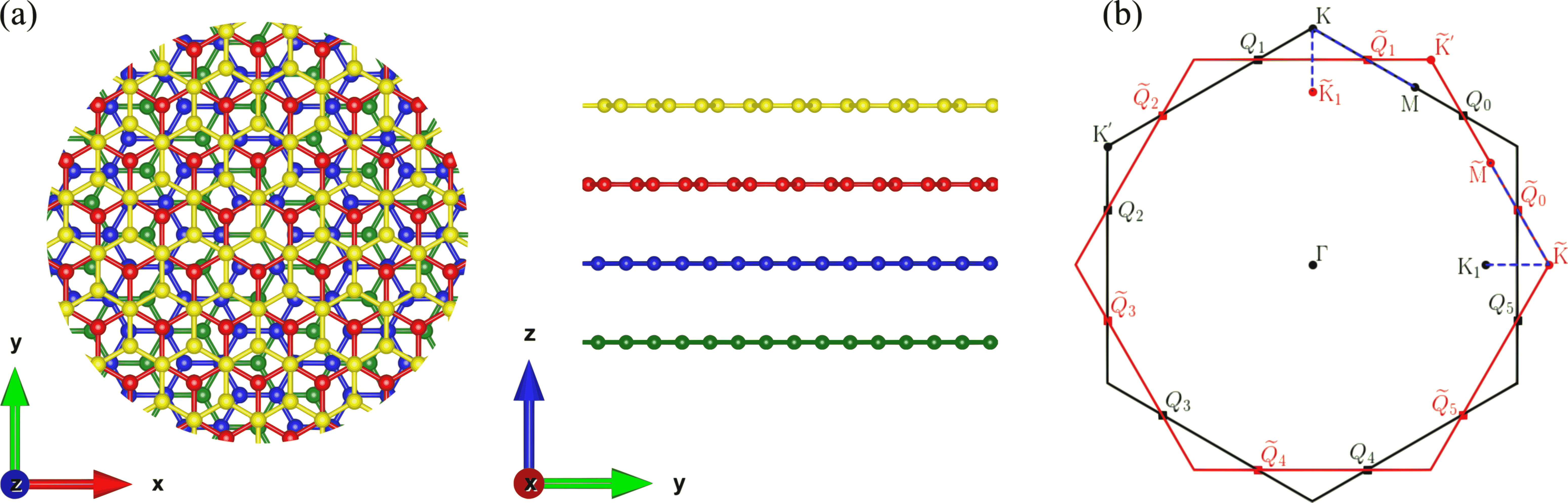
The structure of 30° TDBG is shown in Fig. 1(a). It consists of two AB stacked graphene bilayers with the top bilayer twisted by 30°. The middle two layers form the 30° TBG. So there are two AB stacked interfaces and one 30° twisted interface in 30° TDBG. In this paper, the 30° TDBG is approximated by the 15/26 approximant, which is a periodic Moiré pattern constructed by introducing the slight stress in the top bilayer. The details about the 15/26 approximant are given in Appendix A.

The 30° TDBG and its 15/26 approximant are described by the tight-binding model based on orbitals. The hopping energy between site and is determined bySlater and Koster 1954
| (1) |
where, is the direction cosine of relative position vector with respect to the z axis. The Slater-Koster parameters and have the following forms:
| (2) | |||
| (3) |
The carbon-carbon distance and interlayer distance are chosen to be 3.349 and 1.418 Å, respectively. and are 3.12 and 0.48 eV, respectively. The Fermi velocity and effective band structure calculated using these parameters fit well the experimental results of 30° TBGYu et al. 2019. is a smooth function
| (4) |
This tight-binding model has also been justified by comparing results with several experimentsTrambly de Laissardière et al. 2012; Huder et al. 2018; Shi et al. 2020.
The density of states and optical conductivity are calculated by the tight-binding propagation method (TBPM)Yuan et al. 2010. This method is based on the numerical solution of time-dependent Schrödinger equation without any diagonalization. Both memory and CPU costs scale linearly with the system size. The formula of TBPM are given in Appendix B.
Although the band structure can be derived directly from the periodic 15/26 approximant, its supercell character relative to the primitive unit cell of graphene results in the fold of the bands. So the band structures calculated directly from the 15/26 approximant can not be used to compare with the ARPES measurements. In order to overcome this problem, the band structure of 15/26 approximant is unfolded to the primitive unit cell of graphene. The corresponding formula are given in Appendix C.
III Interlayer decoupling in the low-energy region
First of all, the distributions of the eigenstates in the low energy region are calculated by diagonalizing the Hamiltonian at point and shown in Fig. 2(a). All these states occur inside only the bottom bilayer or top bilayer, which implies the interlayer decoupling between the two bilayer systems in the low energy region. It can be proven further by comparing the band structures and density of states between the 30° TDBG and its subsystem, namely, the AB stacked bilayer graphene (see Fig. 2(b)). Both of them show the parabolic touch point at K point. The good agreement with each other in the vicinity of the Fermi level means that 30° TDBG should has the similar electronic properties to the AB stacked bilayer graphene, such as the optical conductivity shown in Fig. 2(c).
The interlayer decoupling in 30° TDBG can also be proven by checking the Landau levels (see Fig. 3), which is in good agreement with the numerical and analyticalKoshino and Ando 2008 Landau levels of the AB stacked bilayer. In order to compare with the analytical results, a simplified but often used tight-binding approximation is adopted. For the intralayer hoppings, only the nearest-neighbour approximation is adopted. For the interlayer hoppings across the two AB stacked interfaces, only the neighbours stacked vertically are considered. But for the interlayer hoppings across the 30° twisted interface, all the neighbours with the distance less than 5 Å are taken into account. The analytical Landau levels shown in Fig. 3 can be classified into three groups.Koshino and Ando 2008 They are (1) :
| (5) |
(2):
| (6) | ||||
and (3):
| (7) |
In these equations, (labelled by ) stand for the electron and hole bands, respectively. In Fig. 3, only the electron side is shown due to the electron-hole symmetry in this simplified tight-binding model. correspond to the higher and lower subbands in the limit of zero magnetic field, respectively. In the following, we use the notation instead of to avoid the confusion with s = . =0.163 eV (defined by ) is the magnetic energy which corresponds to the Fermi velocity m/s in graphene.
Although the interlayer decoupling dominates the electronic properties in the low-energy region, the obvious interlayer coupling still exist in the high-energy region, especially around point. Actually, 30° TDBG shows the similar electronic structure at all points ( and with i=0, 1, 2, 3, 4 and 5) but deviating from the AB stacked bilayer obviously. It results in the appearance of the new peaks in both density of states and optical conductivity. The origin of the deviation around points will be discussed in the next section.


Similar to 30° TBGYao et al. 2018; Ahn et al. 2018, another important property is the emergence of the energy valley at , which is mirror-symmetric with respect to point (see Fig. 4(a)) because the energy valley at is scattered to with a strong scattering strength . is the interaction between the bottom and top bilayers. and are the Bloch functions of the bottom and top bilayer systems, respectively. The Bloch function of AB stacked bilayer graphene at a general point and sublattice is defined by
| (8) |
Here, is the normalization factor, is the position of sublattice , and is the orbital locating at sublattice in unit cell . The interlayer decoupling and energy valley scattering are robust even an electric field is applied perpendicular to the graphene plane (see Fig. 4(b)).
IV Interlayer coupling at points

The effective band structure of 30° TDBG deviates obviously from the band structure of AB stacked bilayer graphene around points (see Fig. 2(b)), which implies the strong interlayer coupling across the 30° twisted interface. The k-space tight-binding methodMoon et al. 2019 is adopted to understand this phenomenon. In this method, a -related subspace is spanned by Bloch basis functions of both the top and bottom bilayers, namely , and , where () and () are the reciprocal lattice vectors (sublattice) of the bottom and top bilayers, respectively. Actually, only the ’s and ’s with small lengths contribute the Hamiltonian much. In this paper, the 12-wave approximationMoon et al. 2019, namely only considering the ’s and ’s with the length less than , is adopted to construct the Hamiltonian, which has been proven to be accurate enough to simulate the 30° TBG.Moon et al. 2019 The matrix element of the Hamiltonian across the different bilayer systems is
| (9) |
where is the Fourier component of the interlayer hopping function at vector .
Around =0 and under the 12-wave approximation, after folding of the bottom bilayer and of the top bilayer to their corresponding first Brillouin zones, the basis set is just the collection of the Bloch functions of the bottom layer and the Bloch functions of the top bilayer with i=0, 1, 2 3, 4 and 5 (see Fig. 1(b) for their positions). Because there are four sublattices in each bilayer system, the Hamiltonian is a matrix. After the diagonalization of the Hamiltonian, the dispersion relationship between the energy and can be obtained, which is named as quasi-band structure to distinguish the term effective band structure derived by unfolding the band structure of the 15/26 approximant. Due to the energy degeneration of the Bloch states at the 12 points, the strong interactions among them results in the strong deviation of the effective band structure of the 30° TDBG from AB stacked bilayer graphene. In Fig. 5, we plot the quasi-band structure around =0 and compare it with the effective band structure around obtained by band-unfolding method. The good agreement with each other proves the validations of the 12-wave approximation and the 15/26 approximant again. Due to the weaker interaction in the conduction band, we only focus on the electronic structure in the valence band.
At =0, the 24 electronic states in the valence band are labelled by 0, …, 23 (see Fig. 5(a)). Expect for states 0, 11, 12 and 23, the others are all 2-fold degenerate states. The charge distributions of these states are shown in Fig. 6, where (i,j) corresponds to the charge distribution of the 2-fold degenerate states i and j being occupied at the same time. (i,j) or (m,n) means the two charge distributions have the similar pattern and are plotted in the same sub-figure. Comparing with 30° TBG with the symmetry of point group , all the charge distribution patterns in 30° TDBG lose the 12-fold symmetry due to the symmetry decrease to point group . But the corresponding 12-fold-symmetry-like counterparts still exist in 30° TDBG. For example, the occupation number of the charge distribution 0 on the middle two layers is more than 85%. If the occupation on the bottom and top layers is ignored, this charge distribution pattern still possess the 12-fold symmetry, which correspond to the charge distribution or in 30° TBGMoon et al. 2019. Besides, the charge distributions (1,2) and (3,4) have the occupation number on the middle two layers more than 70%, correspond to the cases and in 30° TBGMoon et al. 2019, respectively. The charge distribution (5,6) is similar to the case in 30° TBGMoon et al. 2019, but they show the similar occupation numbers on the four layers. Importantly, all the charge distributions (7,8), (9,10) and 11 show very different charge distribution patterns from the 30° TBG, and these charge distributions have very little occupation number on the middle two layers (less than 20%). These results indicate that the 12-wave interaction results in the strong interlayer coupling between the two bilayer systems at , namely at all points.
V Discussion
During the calculations above, the interlayer distances in both the AB stacked and 30° twisted interfaces are fixed to be 3.349 Å, which may not be their most stable configurations. In order to consider the structure relaxation effect, the interlayer distances in AA, AB stacked and 30° twisted interfaces are determined by classical molucular simulations. The intra- and inter-layer interactions are described by classical REBOBrenner et al. 2002 and Kolmogorov-CrespiKolmogorov and Crespi 2005 potentials, which are implemented in the LAMMPS softwarePlimpton 1995. For a fixed interlayer distance, the atoms are allowed to relax only in plane. The binding energies of the three interfaces at different interlayer distances are given in Fig. 7. At the most stable configurations, the interlayer distances are determined to be 3.61, 3.38 and 3.46 Å for AA, AB stacked and 30° twisted interfaces, respectively, which correspond to the binding energies 13.7, 17.3 and 15.8 meV/atom. Different from the small twist angle, for which the fluctuations of the atoms along the axis introduce the periodic pseudo magnetic field,(Shi et al. 2020) the flatness of the two layers still remains in the 30° twisted interface. After the recalculations by using the relaxed interlayer distances, all the physical conclusions concluded above still be kept.
From the viewpoint of the binding energy, the 30° twisted interface is much more stable than the AA stacked interface and even comparable to the AB stacked one. It means that the 30° twisted interface can be realized easily in experiment. So we also study the effect of the 30° twisted interface between AB stacked bilayer and graphene monolayer (labelled by 30° AB/G), which can be obtained by removing the top layer of the 30° TDBG. Our calculations shown in the Supplemental Materialsm indicate that the interlayer decoupling in the low-energy region and the strong interlayer coupling at points still exist in this system, which implies that it is a general phenomenon in graphene multilayer systems.
VI Conclusion
By means of the tight-binding approximation, we systematically study the electronic properties of 30° TDBG, which are composed of two AB stacked bilayer graphene with top bilayer twisted by 30°. In the low-energy region, the interlayer decoupling across the 30° twisted interface is proven from various electronic properties, such as density of states, effective band structure, optical conductivity and Landau levels. However, the 30° TDBG shows very different effective band structure at points from the AB stacked bilayer due to the 12-wave interaction, which results in the appearance of new van Hove singularities in the density of states and new peaks in the optical conductivity. Importantly, the 12-fold-symmetry-like electronic states, which occur in 30° TBG with exact 12-fold symmetry, can be found in 30° TDBG due to the 12-wave interaction, although its symmetry decreases to point group . Moreover, different from the 30° TBG, some special electronic states appear, which have large occupation number on the top and bottom layers but little occupation nunber on the middle two layers. These results imply that the strong interlayer coupling still exist across the 30° twist in 30° TDBG, especially at points, although it shows interlayer decoupling in the vicinity of the Fermi level.
ACKNOWLEDGEMENTS
This work is supported by the National Science Foundation of China (Grant No. 11774269) and China Postdoctoral Science Foundation (Grant No. 2018M632902). MIK acknowledges a support by the JTC-FLAGERA Project GRANSPORT. Numerical calculations presented in this paper have been partially performed on the supercomputing system in the Supercomputing Center of Wuhan University. Support by the Netherlands National Computing Facilities foundation (NCF), with funding from the Netherlands Organisation for Scientific Research (NWO), is gratefully acknowledged.
Appendix A 15/26 approximant
We follow the procedure proposed for 30° TBGYu et al. 2019 to construct the approximant of 30° TDBG. That is, the bottom bilayer keeps the lattice constant of a pristine graphene Å, but the top bilayer is slightly compressed with the lattice constant changing to be Å, which makes the two bilayers become commensurate. The resulting periodic pattern is used as the approximant, which is named as 15/26 approximant due to the commensurate period along the direction, where and are the basic periods of the bottom and top bilayers, respectively. Accordingly, the elementary unit cell of the 15/26 approximant contains 13502 and 13522 sites in the bottom and top bilayers, respectively. Our results given in the Supplemental Materialsm indicate that the 15/26 approximant can reproduce the density of states and the optical conductivity of 30° TDBG accurately.
Appendix B Tight-binding propagation method
In TBPMYuan et al. 2010, a random superposition of the orbitals at all sites is used as the initial state with . DOS is calculated as Fourier transform of the time-dependent correlation function
| (10) |
The optical conductivity is calculated by using the Kubo formula in TBPMYuan et al. 2010. The real part of the optical conductivity matrix at temperature reads
| (11) | |||
Here, is the area of the unit cell per layer, and wave functions
| (12) | |||
where is the Fermi-Dirac distribution operator, where is the electronic chemical potential.
Appendix C effective band structure
First of all, the spectral function at wavevector and energy can be calculated byNishi et al. 2017
| (13) |
where is the energy for band at wavevector for the approximant. Actually, only one , namely being the reciprocal lattice vector of the approximant, contributes to the spectral function. The spectral weight is defined as
| (14) |
where and are the eigenstates of layer and the approximant, respectively. Under the tight-binding method, the spectral weight contributed from layer can be described by
| (15) |
Here, is the number of primitive unit cell of layer in one elementary unit cell of the approximant. is the projection of (the eigenstate of the approximant) on (the Bloch basis function of approximant). Equation (15) indicates that only the eigenstates of approximant are necessary to obtain the spectral function.
Then, the effective band structure can be obtained byMedeiros et al. 2014
| (16) |
where is the bin width in energy sampling.
References
- Shallcross et al. (2010) S. Shallcross, S. Sharma, E. Kandelaki, and O. A. Pankratov, Phys. Rev. B 81, 165105 (2010).
- Berger et al. (2006) C. Berger, Z. Song, X. Li, X. Wu, N. Brown, C. Naud, D. Mayou, T. Li, J. Hass, A. N. Marchenkov, E. H. Conrad, P. N. First, and W. A. de Heer, Science 312, 1191 (2006).
- Hass et al. (2008) J. Hass, F. Varchon, J. E. Millán-Otoya, M. Sprinkle, N. Sharma, W. A. de Heer, C. Berger, P. N. First, L. Magaud, and E. H. Conrad, Phys. Rev. Lett. 100, 125504 (2008).
- Miller et al. (2009) D. L. Miller, K. D. Kubista, G. M. Rutter, M. Ruan, W. A. de Heer, P. N. First, and J. A. Stroscio, Science 324, 924 (2009).
- Sadowski et al. (2006) M. L. Sadowski, G. Martinez, M. Potemski, C. Berger, and W. A. de Heer, Phys. Rev. Lett. 97, 266405 (2006).
- Sprinkle et al. (2009) M. Sprinkle, D. Siegel, Y. Hu, J. Hicks, A. Tejeda, A. Taleb-Ibrahimi, P. Le Fèvre, F. Bertran, S. Vizzini, H. Enriquez, S. Chiang, P. Soukiassian, C. Berger, W. A. de Heer, A. Lanzara, and E. H. Conrad, Phys. Rev. Lett. 103, 226803 (2009).
- de Heer et al. (2010) W. A. de Heer, C. Berger, X. Wu, M. Sprinkle, Y. Hu, M. Ruan, J. A. Stroscio, P. N. First, R. Haddon, B. Piot, C. Faugeras, M. Potemski, and J.-S. Moon, Journal of Physics D: Applied Physics 43, 374007 (2010).
- Sprinkle et al. (2010) M. Sprinkle, J. Hicks, A. Tejeda, A. Taleb-Ibrahimi, P. L. Fèvre, F. Bertran, H. Tinkey, M. C. Clark, P. Soukiassian, D. Martinotti, J. Hass, and E. H. Conrad, Journal of Physics D: Applied Physics 43, 374006 (2010).
- van Wijk et al. (2015) M. M. van Wijk, A. Schuring, M. I. Katsnelson, and A. Fasolino, 2D Materials 2, 034010 (2015).
- Suárez Morell et al. (2010a) E. Suárez Morell, J. D. Correa, P. Vargas, M. Pacheco, and Z. Barticevic, Phys. Rev. B 82, 121407 (2010a).
- Yin et al. (2015) L.-J. Yin, J.-B. Qiao, W.-X. Wang, W.-J. Zuo, W. Yan, R. Xu, R.-F. Dou, J.-C. Nie, and L. He, Phys. Rev. B 92, 201408 (2015).
- Suárez Morell et al. (2010b) E. Suárez Morell, J. D. Correa, P. Vargas, M. Pacheco, and Z. Barticevic, Phys. Rev. B 82, 121407 (2010b).
- Bistritzer and MacDonald (2011) R. Bistritzer and A. H. MacDonald, Proceedings of the National Academy of Sciences 108, 12233 (2011).
- Cao et al. (2018a) Y. Cao, V. Fatemi, S. Fang, K. Watanabe, T. Taniguchi, E. Kaxiras, and P. Jarillo-Herrero, Nature 556, 43 (2018a), article.
- Po et al. (2018) H. C. Po, L. Zou, A. Vishwanath, and T. Senthil, Phys. Rev. X 8, 031089 (2018).
- Yankowitz et al. (2019) M. Yankowitz, S. Chen, H. Polshyn, Y. Zhang, K. Watanabe, T. Taniguchi, D. Graf, A. F. Young, and C. R. Dean, Science 363, 1059 (2019).
- Cao et al. (2018b) Y. Cao, V. Fatemi, A. Demir, S. Fang, S. L. Tomarken, J. Y. Luo, J. D. Sanchez-Yamagishi, K. Watanabe, T. Taniguchi, E. Kaxiras, R. C. Ashoori, and P. Jarillo-Herrero, Nature 556, 80 (2018b).
- Ahn et al. (2018) S. J. Ahn, P. Moon, T.-H. Kim, H.-W. Kim, H.-C. Shin, E. H. Kim, H. W. Cha, S.-J. Kahng, P. Kim, M. Koshino, Y.-W. Son, C.-W. Yang, and J. R. Ahn, Science 361, 782 (2018).
- Yao et al. (2018) W. Yao, E. Wang, C. Bao, Y. Zhang, K. Zhang, K. Bao, C. K. Chan, C. Chen, J. Avila, M. C. Asensio, J. Zhu, and S. Zhou, Proceedings of the National Academy of Sciences 115, 6928 (2018).
- Takesaki et al. (2016) Y. Takesaki, K. Kawahara, H. Hibino, S. Okada, M. Tsuji, and H. Ago, Chemistry of Materials 28, 4583 (2016).
- Pezzini et al. (0) S. Pezzini, V. Mišeikis, G. Piccinini, S. Forti, S. Pace, R. Engelke, F. Rossella, K. Watanabe, T. Taniguchi, P. Kim, and C. Coletti, Nano Letters 0, null (0), pMID: 32297749, https://doi.org/10.1021/acs.nanolett.0c00172 .
- Deng et al. (2020a) B. Deng, B. Wang, N. Li, R. Li, Y. Wang, J. Tang, Q. Fu, Z. Tian, P. Gao, J. Xue, and H. Peng, ACS Nano 14, 1656 (2020a).
- Lin et al. (2018) Y. R. Lin, N. Samiseresht, M. Franke, S. Parhizkar, S. Soubatch, B. Amorim, T. L. Lee, C. Kumpf, F. S. Tautz, and F. C. Bocquet, arXiv e-prints , arXiv:1809.07958 (2018).
- Park et al. (2019) M. J. Park, H. S. Kim, and S. Lee, Phys. Rev. B 99, 245401 (2019).
- Koren and Duerig (2016) E. Koren and U. Duerig, Phys. Rev. B 93, 201404 (2016).
- Suzuki et al. (2019) T. Suzuki, T. Iimori, S. J. Ahn, Y. Zhao, M. Watanabe, J. Xu, M. Fujisawa, T. Kanai, N. Ishii, J. Itatani, K. Suwa, H. Fukidome, S. Tanaka, J. R. Ahn, K. Okazaki, S. Shin, F. Komori, and I. Matsuda, ACS Nano 13, 11981 (2019).
- Moon et al. (2019) P. Moon, M. Koshino, and Y.-W. Son, Phys. Rev. B 99, 165430 (2019).
- Yan et al. (2019a) C. Yan, D. Ma, J. Qiao, H. Zhong, L. Yang, S.-Y. Li, Z. Fu, Y. Zhang, and L. He, 2D Materials (2019a).
- Yu et al. (2019) G. Yu, Z. Wu, Z. Zhan, M. I. Katsnelson, and S. Yuan, npj Computational Materials 5, 122 (2019).
- Yan et al. (2019b) C. Yan, D.-L. Ma, J.-B. Qiao, H.-Y. Zhong, L. Yang, S.-Y. Li, Z.-Q. Fu, Y. Zhang, and L. He, 2D Materials 6, 045041 (2019b).
- Deng et al. (2020b) B. Deng, B. Wang, N. Li, R. Li, Y. Wang, J. Tang, Q. Fu, Z. Tian, P. Gao, J. Xue, and H. Peng, ACS Nano 14, 1656 (2020b).
- Liu et al. (2019) X. Liu, Z. Hao, E. Khalaf, J. Y. Lee, K. Watanabe, T. Taniguchi, A. Vishwanath, and P. Kim, arXiv e-prints , arXiv:1903.08130 (2019).
- Cao et al. (2019) Y. Cao, D. Rodan-Legrain, O. Rubies-Bigordà, J. M. Park, K. Watanabe, T. Taniguchi, and P. Jarillo-Herrero, arXiv e-prints , arXiv:1903.08596 (2019).
- Scheurer et al. (2019) M. S. Scheurer, R. Samajdar, and S. Sachdev, arXiv e-prints , arXiv:1906.03258 (2019).
- Shen et al. (2020) C. Shen, Y. Chu, Q. Wu, N. Li, S. Wang, Y. Zhao, J. Tang, J. Liu, J. Tian, K. Watanabe, T. Taniguchi, R. Yang, Z. Y. Meng, D. Shi, O. V. Yazyev, and G. Zhang, Nature Physics (2020), 10.1038/s41567-020-0825-9.
- Burg et al. (2019) G. W. Burg, J. Zhu, T. Taniguchi, K. Watanabe, A. H. MacDonald, and E. Tutuc, Phys. Rev. Lett. 123, 197702 (2019).
- Haddadi et al. (2020) F. Haddadi, Q. Wu, A. J. Kruchkov, and O. V. Yazyev, Nano Letters 20, 2410 (2020).
- Chebrolu et al. (2019) N. R. Chebrolu, B. L. Chittari, and J. Jung, Phys. Rev. B 99, 235417 (2019).
- Choi and Choi (2019) Y. W. Choi and H. J. Choi, Phys. Rev. B 100, 201402 (2019).
- Koshino (2019) M. Koshino, Phys. Rev. B 99, 235406 (2019).
- Liu et al. (2019) J. Liu, Z. Ma, J. Gao, and X. Dai, Phys. Rev. X 9, 031021 (2019).
- Brown et al. (2012) L. Brown, R. Hovden, P. Huang, M. Wojcik, D. A. Muller, and J. Park, Nano Letters 12, 1609 (2012).
- Wu et al. (2016) J.-B. Wu, H. Wang, X.-L. Li, H. Peng, and P.-H. Tan, Carbon 110, 225 (2016).
- Slater and Koster (1954) J. C. Slater and G. F. Koster, Phys. Rev. 94, 1498 (1954).
- Trambly de Laissardière et al. (2012) G. Trambly de Laissardière, D. Mayou, and L. Magaud, Phys. Rev. B 86, 125413 (2012).
- Huder et al. (2018) L. Huder, A. Artaud, T. Le Quang, G. T. de Laissardière, A. G. M. Jansen, G. Lapertot, C. Chapelier, and V. T. Renard, Phys. Rev. Lett. 120, 156405 (2018).
- Shi et al. (2020) H. Shi, Z. Zhan, Z. Qi, K. Huang, E. v. Veen, J. Á. Silva-Guillén, R. Zhang, P. Li, K. Xie, H. Ji, M. I. Katsnelson, S. Yuan, S. Qin, and Z. Zhang, Nature Communications 11, 371 (2020).
- Yuan et al. (2010) S. Yuan, H. De Raedt, and M. I. Katsnelson, Phys. Rev. B 82, 115448 (2010).
- Koshino and Ando (2008) M. Koshino and T. Ando, Phys. Rev. B 77, 115313 (2008).
- Brenner et al. (2002) D. W. Brenner, O. A. Shenderova, J. A. Harrison, S. J. Stuart, B. Ni, and S. B. Sinnott, Journal of Physics: Condensed Matter 14, 783 (2002).
- Kolmogorov and Crespi (2005) A. N. Kolmogorov and V. H. Crespi, Phys. Rev. B 71, 235415 (2005).
- Plimpton (1995) S. Plimpton, Journal of Computational Physics 117, 1 (1995).
- (53) See Supplemental Material at link for SI. The validation of 15/26 approximant. SII. The interlayer decoupling in 30° AB/G. SIII. The interlayer coupling at Q points in 30° AB/G.
- Nishi et al. (2017) H. Nishi, Y.-i. Matsushita, and A. Oshiyama, Phys. Rev. B 95, 085420 (2017).
- Medeiros et al. (2014) P. V. C. Medeiros, S. Stafström, and J. Björk, Phys. Rev. B 89, 041407 (2014).