Multi-messenger tests of cosmic-ray acceleration
in radiatively inefficient accretion flows
Abstract
The cores of active galactic nuclei (AGNs) have been suggested as the sources of IceCube neutrinos, and recent numerical simulations have indicated that hot AGN coronae of Seyfert galaxies and radiatively inefficient accretion flows (RIAFs) of low-luminosity AGNs (LLAGNs) may be promising sites of ion acceleration. We present detailed studies on detection prospects of high-energy multi-messenger emissions from RIAFs in nearby LLAGNs. We construct a model of RIAFs that can reproduce the observational features of the current X-ray observations of nearby LLAGNs. We then calculate the high-energy particle emissions from nearby individual LLAGNs, including MeV gamma rays from thermal electrons, TeV–PeV neutrinos produced by non-thermal protons, and sub-GeV to sub-TeV gamma rays from proton-induced electromagnetic cascades. We find that, although these are beyond the reach of current facilities, proposed future experiments such as e-ASTROGAM and IceCube-Gen2 should be able to detect the MeV gamma rays and the neutrinos, respectively, or else they can place meaningful constraints on the parameter space of the model. On the other hand, the detection of high-energy gamma rays due to the electromagnetic cascades will be challenging with the current and near-future experiments, such as Fermi and Cherenkov Telescope Array. In an accompanying paper, we demonstrate that LLAGNs can be a source of the diffuse soft gamma-ray and TeV–PeV neutrino backgrounds, whereas in the present paper, we focus on the prospects for multi-messenger tests which can be applied to reveal the nature of the high-energy neutrinos and photons from LLAGNs.
I Introduction
The IceCube Collaboration reported the detection of extraterrestrial neutrinos in 2013 Aartsen et al. 2013; IceCube Collaboration 2013 and provided the details of the diffuse neutrino background intensity Aartsen et al. 2014; Aartsen et al. 2015a; Aartsen et al. 2015b. The origin of the astrophysical neutrino background has yet to be confirmed (see Ref. Ahlers and Halzen 2017 for a review). Gamma-ray bursts (GRBs) were expected to be a promising neutrino source Waxman and Bahcall 1997; Mészáros and Waxman 2001; Dermer and Atoyan 2003; Guetta et al. 2004; Murase and Nagataki 2006a. However, stacking analyses using the information of the observed GRBs detect no associated neutrinos, which puts an upper limit on the GRB contribution to the neutrino intensity of % Aartsen et al. 2016; Aartsen et al. 2017. Note that these analyses focus on the prompt emission from bright GRBs, while neutrinos produced in the afterglow phase Waxman and Bahcall 2000; Murase and Nagataki 2006b; Murase 2007; Kimura et al. 2017, by low-luminosity GRBs and engine-driven supernovae Murase et al. 2006; Senno et al. 2016; Zhang et al. 2018; Boncioli et al. 2019; Zhang and Murase 2018, or by failed GRBs (also known as choked jets; Mészáros and Waxman 2001; Razzaque et al. 2003; Ando and Beacom 2005; Horiuchi and Ando 2008; Murase and Ioka 2013; He et al. 2018; Denton and Tamborra 2018; Kimura et al. 2018) are not very constrained.
Blazars are also believed to be capable of strong neutrino emission Mannheim et al. 1992; Halzen and Zas 1997; Atoyan and Dermer 2001. Recently, IceCube reported the detection of a high-energy neutrino coincident with a flaring activity of a blazar, TXS 0506+056 IceCube-Collaboration et al. 2018. Thanks to the ensuing multi-messenger followup campaign (see Aartsen et al. 2017a), the broad-band spectral energy distribution during the flaring period has been determined, which enables one to model the neutrino emission in detail Keivani et al. 2018; Murase et al. 2018; Liu et al. 2018; Cerruti et al. 2019; Gao et al. 2019. The IceCube Collaboration also found a neutrino flare from this object during 2014 – 2015, by re-analyzing their archival data IceCube-Collaboration 2018. However, this neutrino flare is not accompanied by a corresponding GeV gamma-ray flaring activity Garrappa et al. 2019, which challenges the theoretical modeling of the neutrino emission Murase et al. 2018; Reimer et al. 2018; Rodrigues et al. 2018; Wang et al. 2018. Note that the coincident detection and the archival neutrino flare do not, however, mean that the blazars are the dominant source of the diffuse neutrinos. The stacking analyses of the blazars detected by Fermi result in a non-detection Aartsen et al. 2017b; Neronov et al. 2017; Yuan et al. 2019; Hooper et al. 2019, which implies that their contribution is less than % of the total astrophysical neutrinos. Also, the absence of event clustering in the arrival distribution of neutrinos indicates that the contributions from flaring blazars should be less than % Murase and Waxman 2016; Murase et al. 2018.
Another constraint is provided by the extragalactic gamma-ray background detected by Fermi Ackermann et al. 2015. When astrophysical neutrinos are produced through pion decay, gamma rays are also produced simultaneously. The generated gamma-ray luminosity is comparable to the neutrino luminosity, and the TeV–PeV gamma rays are cascaded down to the GeV–TeV energy range during their propagation towards Earth. In order to avoid overproducing the observed extragalactic gamma-ray background, the neutrino spectral index should be smaller than Murase et al. 2013, which is in tension with the best-fit spectrum of the observed neutrinos in the shower analyses Aartsen et al. 2015b; Aartsen et al. 2015a; Aartsen et al. 2015; Aartsen et al. 2017c. Also, the neutrino flux at 1–100 TeV is higher than that above 100 TeV Aartsen et al. 2015a; Aartsen et al. 2015b, although this might be due to the strong atmospheric background Palladino and Winter 2018. If such a “medium-energy excess” is real, the serious tension with the gamma-ray background is unavoidable, suggesting that the main sources are opaque and hidden in high-energy gamma rays Murase et al. 2016. This argument disfavors many astrophysical scenarios as the origin of these neutrinos, including starburst galaxies Loeb and Waxman 2006; Murase et al. 2013; He et al. 2013; Anchordoqui et al. 2014; Liu et al. 2014; Tamborra et al. 2014; Senno et al. 2015; Xiao et al. 2016; Bechtol et al. 2017; Sudoh et al. 2018, galaxy clusters Murase et al. 2008; Kotera et al. 2009; Murase et al. 2013; Zandanel et al. 2015; Fang and Olinto 2016; Fang and Murase 2018, and radio-galaxies Becker Tjus et al. 2014; Hooper 2016.
We consider high-energy neutrino emission from the vicinity of supermassive black holes (SMBHs) in active galactic nuclei (AGNs) Berezinskii and Ginzburg 1981; Kazanas and Ellison 1986; Zdziarski 1986; Begelman et al. 1990; Stecker et al. 1991; Bednarek and Protheroe 1999; Alvarez-Muñiz and Mészáros 2004. A luminous AGN hosts a geometrically thin, optically thick accretion disk that produces copious UV photons Shakura and Sunyaev 1973; Malkan 1983; Czerny and Elvis 1987, and the ratio of the observed UV to X-ray luminosity is very high Marconi et al. 2004; Hopkins et al. 2007; Lusso et al. 2012. Such target photon fields lead to a hard neutrino spectrum at PeV energies Kalashev et al. 2015; Inoue et al. 2019. The accretion shock has been considered, but the existence of such a shock has not been supported by numerical simulations so far. On the other hand, recent studies on magnetorotational instabilities suggest that particle acceleration via magnetic reconnections and turbulence is promising in AGN coronae, and Ref. Murase et al. 2019a showed that the mysterious 10 – 100 TeV component in the diffuse neutrino flux can be explained by the AGN core model of radio-quiet AGNs. It was found that the Bethe-Heitler process is critically important, which led to robust predictions of MeV gamma rays via proton-induced cascades.
Low-luminosity AGNs (LLAGNs), however, have different spectral energy distributions, in which an UV bump is absent Ho 2008. This indicates that there is an optically thin, hot accretion flow instead of an optically thick disk. Remarkably, plasma properties of hot AGN coronae and radiatively inefficient accretion flows (RIAF; Narayan and Yi 1994; Yuan and Narayan 2014) in LLAGNs seem similar in the sense that the plasmas are expected to be collisionless for ions. It is natural to consider the same type of proton acceleration in both Seyfert galaxies and LLAGNs. Ref. Kimura et al. 2015 considered the stochastic acceleration expected in such RIAFs of LLAGNs, and showed that the neutrinos produced by the accelerated protons can account for the diffuse astrophysical neutrino background (see also Refs. Khiali and de Gouveia Dal Pino 2016; Righi et al. 2019 for neutrino emissions from LLAGNs). The LLAGN model can avoid the gamma-ray and the point-source constraints, thanks to its compact emission region and high number density, although Ref. Kimura et al. 2015 did not provide details of the resulting gamma-ray spectra.
In this paper, we describe a refined LLAGN model, and show how multi-messenger information on neutrinos and gamma rays can be used as a test of the proposed LLAGN model. We estimate the physical quantities in the RIAFs of several nearby LLAGNs including the photons from the thermal electrons in Section II. We then estimate the high-energy proton spectra in Section III, and calculate the high-energy neutrino spectra and their detectability in Section IV. We calculate the gamma rays from proton-induced electromagnetic cascades in Section V. Finally, we summarize the results and discuss their implications in Section VI. We note that our refined model can reproduce the diffuse MeV gamma-ray and the TeV – PeV neutrino backgrounds simultaneously without overshooting the Fermi data, which is shown in an accompanying paper. In this paper, we focus on the detection prospects of individual nearby LLAGNs.
II Physical quantities in RIAFs
We consider a RIAF of size and mass accretion rate around a SMBH of mass . We use the notation in cgs units, unless otherwise noted. To represent the physical quantities in the RIAF, it is convenient to normalize by the Schwarzschild radius: , where is the Schwarzschild radius, is the gravitational constant, and is the speed of light. The mass accretion rate is normalized by the Eddington accretion rate: , where is the Eddington luminosity.
According to recent magnetohydrodynamic (MHD) simulations (see e.g., Refs. Machida and Matsumoto 2003; McKinney 2006; Ohsuga and Mineshige 2011; Narayan et al. 2012; Penna et al. 2013; Kimura et al. 2019), the radial velocity, the sound velocity, the scale height, the number density, the magnetic field, and the Alfven velocity in the RIAF are estimated to be
where is the Keplerian velocity, is the viscous parameter Shakura and Sunyaev 1973, is the proton mass, is the plasma beta, and is the gas pressure. We assume pure proton composition for simplicity. The magnetic field strength in the hot accretion flows depends on the configuration of the magnetic field: for standard and normal evolution (SANE) flows, whereas for magnetically arrested disks (e.g., McKinney 2006; Narayan et al. 2012; Ressler et al. 2017; Chael et al. 2018). We use as a reference value because lower plasma are suitable for producing non-thermal particles Ball et al. 2018. For the viscous parameter , SANE models tend to give a lower value, Penna et al. 2013; Kimura et al. 2019, while observations of X-ray binaries and dwarf novae suggest (see Ref. Martin et al. 2019 and references therein). Here, we set as a reference value.
Although cooling processes have little influence on the dynamical structure in the RIAF, the thermal electrons supply target photons for photohadronic interactions and two-photon annihilation. We calculate the characteristics of the target photons in the RIAF using a method similar to Ref. Kimura et al. 2015. We consider synchrotron, bremsstrahlung, and inverse Compton emission processes. The calculation method of the emission spectrum due to each process was discussed in the Appendix of Ref. Kimura et al. 2015. Note that this treatment is valid only for flows with Thomson optical depths , where is the Thomson cross section.
As long as , the balance between the cooling rate and heating rate of the thermal electrons determines the electron temperature, , where is the electron mass and is the Boltzmann constant Xie and Yuan 2012; Yuan and Narayan 2014. Then, the electron heating rate is equal to the bolometric luminosity from the thermal electrons. If the Coulomb collisions with the thermal protons are the dominant heating process, the heating rate is proportional to , which leads to . Then, the bolometric luminosity is phenomenologically given by (see, e.g., Ref. Mahadevan and Quataert 1997; Kato et al. 2008)
| (1) |
where is the normalized critical accretion rate above which the RIAF solution no longer exists Narayan and Yi 1995; Abramowicz et al. 1995 and is the radiation efficiency of the standard thin disk. The critical accretion rate can be expressed as a function of Mahadevan 1997; Xie and Yuan 2012. Following Ref. Mahadevan 1997, we represent . Note that the dissipation processes in collisionless accretion flows are still controversial. If the electrons are directly heated by plasma dissipation processes induced by kinetic instabilities Quataert and Gruzinov 1999; Sharma et al. 2007; Riquelme et al. 2012; Kunz et al. 2014; Hoshino 2013; Hoshino 2015; Sironi and Narayan 2015; Sironi 2015; Zhdankin et al. 2018, the electron heating rate may be proportional to , leading to as assumed in Ref. Kimura et al. 2015. In reality, the scaling relation may be located between the two regimes. In this paper, we use Equation (1) for simplicity.
Observations give us the X-ray luminosity, , which is connected to in our model. Using the bolometric correction factor, , the X-ray luminosity is related to the bolometric luminosity as
| (2) |
According to the X-ray surveys, is higher for a higher or , where is the Eddington ratio. At the low-luminosity end, becomes almost constant, Wang et al. 2004; Lusso et al. 2012; Liu et al. 2016. Using Equations (1) and (2) with a constant , we can write as a function of observables:
| (3) |
where we use and . This is less than . Hence, typical LLAGNs with can host RIAFs.
We calculate spectral energy distributions of nearby LLAGNs listed in Table A.3 of Ref. Saikia et al. 2018, which provides , , luminosity distance (), and declination angle () for 70 LLAGNs. The mass accretion rate of the listed LLAGNs is estimated using Equation (3) with . We find that 7 of them have standard disks, i.e., , while the others host RIAFs. Figure 1 shows the target photon spectra from 4 LLAGNs whose parameters and resulting physical quantities are tabulated in Table 1 and 2, respectively. The values of the other parameters are tabulated in Table 3. The four LLAGNs differ in and . NGC 3516, NGC 4203, and NGC 5866 have close to , while NGC 3998 hosts a SMBH of . is close to the critical accretion rate for NGC 3516, for NGC 4203 and NGC 3998, and for NGC 5866. For all the LLAGNs, the synchrotron emission peaks in the radio band. For LLAGNs with , the inverse Compton emission of the synchrotron photons produces infrared to MeV photons. For lower cases, the bremsstrahlung emits MeV photons due to inefficient Comptonization. The inverse Compton emission spectrum is hard and smooth for higher , while it is soft and bumpy for lower due to a high value of electron temperature and a low value of Compton- parameter, (see Table 1 for the values of , , and ). A high value of with fixed lowers the peak frequency of the synchrotron emission due to the weak magnetic field, and increases the entire luminosity because of a high net accretion luminosity, .
Next, we compare the X-ray luminosities obtained by our calculations and observations. Figure 2 shows the relation between the observed keV X-ray luminosity, , and the X-ray luminosity calculated by our model, in the same band. Intriguingly, our simple model is in a good agreement with the observations for . The two luminosities match within a factor of 1.7 in this sample. We stress that we do not adjust the X-ray luminosity but we calculate photon spectra with the one-zone model using estimated by Equations (2) and (3). For a lower value of , the synchrotron emission is more efficient than the inverse Compton emission. This causes a higher value of , resulting in as seen in the figure. For nearby low-ionization nuclear emission-like regions (LINERs), the bolometric correction factor is estimated to be Eracleous et al. 2010. is higher with such a higher value of , since it leads to a higher value of . Hence, a higher value of is more consistent with our model with . Nevertheless, we use because LLAGNs with do not affect the detectability of high-energy neutrinos as shown in Section IV.
The bright LLAGNs are detected by the Swift BAT, most of which show hard X-ray spectra. Thus, very interestingly, our model is consistent with the BAT data in terms of luminosity. In addition, RIAF models generally predict that a higher object has a harder photon spectrum in the X-ray band owing to a higher value of the Compton- parameter, which is consistent with the observed anti-correlation between the X-ray spectral index and the Eddington ratio Gu and Cao 2009; She et al. 2018.
Recently, Ref. Younes et al. 2019 estimated the cutoff energy in X-ray spectrum in NGC 3998 to be around 100 keV using the NuSTAR and XMM-Newton data. However, they just measured a slight softening of the spectrum, which can be reconciled by our RIAF model. The Compton scattering makes a few bumps in the broad-band spectrum, which causes a softening in the X-ray band for NGC 3998 as seen in Figure 1. Here, we do not compare our model to observations in detail, because they are beyond the scope of this paper.
In order to obtain the electron temperature more concretely, we need to detect a clear cutoff feature above 100 keV. We plot the photon spectra due to thermal electrons above 10 keV with the sensitivity curve of the proposed future satellite, e-ASTROGAM De Angelis et al. 2017 in Figure 3. The MeV gamma rays will be easily detected for NGC 3516 and NGC 4258, although it is not expected for NGC 3031. The other proposed MeV gamma-ray satellites, AMEGO Moiseev and Amego Team 2017 and GRAMS Aramaki et al. 2020, have similar or better sensitivity in this range. The MeV observations of nearby LLAGNs will provide not only the electron temperature in RIAFs for the first time, but also the crucial test for the LLAGN contribution to the MeV gamma-ray background (see the accompanying paper).
| ID | Type | |||||
|---|---|---|---|---|---|---|
| NGC | [erg s-1 cm-2] | [erg s-1] | [] | [Mpc] | [deg] | |
| 4565 | S1.9 | -10.73 | 41.32 | 7.43 | 9.7 | 26.0 |
| 3516 | S1.2 | -10.84 | 42.42 | 8.07 | 38.9 | 72.6 |
| 4258 | S1.9 | -10.84 | 40.90 | 7.62 | 6.8 | 47.3 |
| 3227 | S1.5 | -11.06 | 41.64 | 7.43 | 20.6 | 19.9 |
| 4138 | S1.9 | -11.26 | 41.28 | 7.17 | 17.0 | 43.7 |
| 3169 | L2 | -11.32 | 41.35 | 8.16 | 19.7 | 3.5 |
| 4579 | S1.9/L | -11.36 | 41.17 | 7.86 | 16.8 | 11.8 |
| 3998 | L1.2 | -11.43 | 41.32 | 9.23 | 21.6 | 55.5 |
| 3718 | L1.9 | -11.48 | 41.06 | 7.77 | 17.0 | 53.1 |
| 4203 | L1.9 | -11.68 | 40.37 | 7.89 | 9.7 | 33.2 |
| 4486 | L2 | -11.71 | 40.82 | 9.42 | 16.8 | 12.4 |
| 3031 | S1.5 | -11.71 | 39.48 | 7.82 | 3.6 | 69.1 |
| 5866 | T2 | -14.16 | 38.29 | 7.92 | 15.3 | 55.8 |
| ID | |||||||||
|---|---|---|---|---|---|---|---|---|---|
| NGC | [cm] | [cm-3] | [G] | [MeV] | [erg s-1] | [%] | |||
| 4565 | -1.78 | 13.90 | 9.45 | 2.81 | -0.83 | 1.09 | 2.78 | 41.23/41.05/41.74 | 10/6/37 |
| 3516 | -1.55 | 14.54 | 9.04 | 2.61 | -0.60 | 0.93 | 2.22 | 42.10/41.92/42.61 | 8/4/29 |
| 4258 | -2.08 | 14.09 | 8.96 | 2.57 | -1.13 | 1.39 | 3.50 | 41.11/40.94/41.63 | 12/8/44 |
| 3227 | -1.62 | 13.90 | 9.61 | 2.89 | -0.67 | 0.96 | 2.39 | 41.39/41.21/41.90 | 9/5/32 |
| 4138 | -1.67 | 13.64 | 9.82 | 3.00 | -0.72 | 0.99 | 2.51 | 41.08/40.90/41.59 | 9/6/34 |
| 3169 | -2.13 | 14.63 | 8.37 | 2.27 | -1.18 | 1.47 | 3.63 | 41.61/41.43/42.13 | 12/8/44 |
| 4579 | -2.07 | 14.33 | 8.73 | 2.45 | -1.12 | 1.39 | 3.48 | 41.37/41.19/41.89 | 12/8/43 |
| 3998 | -2.68 | 15.70 | 6.75 | 1.46 | -1.73 | 2.25 | 4.52 | 42.13/41.95/42.65 | 14/10/50 |
| 3718 | -2.08 | 14.24 | 8.81 | 2.49 | -1.13 | 1.39 | 3.50 | 41.27/41.09/41.79 | 12/8/43 |
| 4203 | -2.48 | 14.36 | 8.29 | 2.23 | -1.53 | 1.84 | 4.12 | 40.98/40.81/41.51 | 14/9/49 |
| 4486 | -3.02 | 15.89 | 6.22 | 1.20 | -2.07 | 2.74 | 5.56 | 41.97/41.80/42.50 | 15/10/52 |
| 3031 | -2.89 | 14.29 | 7.95 | 2.06 | -1.94 | 2.30 | 5.14 | 40.50/40.33/41.03 | 15/10/52 |
| 5866 | -3.54 | 14.39 | 7.20 | 1.69 | -2.59 | 2.85 | 5.89 | 39.96/39.82/40.58 | 16/12/66 |
Common parameters
| 0.1 | 3.2 | 10 | 15 | 0.1 |
Model-dependent parameters and quantities Parameters Model A 3.0 7.5 1.666 - - Model B 2.0 - - 1.0 Model C 0.010 - - 2.0


III Non-thermal Protons in RIAFs
High-energy protons may be accelerated and injected into RIAFs by magnetic reconnections Zenitani and Hoshino 2001; Kowal et al. 2012; Sironi and Spitkovsky 2014; Hoshino 2015; Kunz et al. 2016; Ball et al. 2018, stochastic acceleration via MHD turbulence Kimura et al. 2016; Comisso and Sironi 2018; Kimura et al. 2019; Wong et al. 2019, or electric potential gaps in the black hole magnetosphere Chen et al. 2018; Levinson and Cerutti 2018. We examine three cases of non-thermal proton spectra. One is the stochastic acceleration model (model A), in which we solve the diffusion equation in momentum space. The others are the power-law injection models (models B and C) in which we consider an injection term with a single power-law with an exponential cutoff. Such a power-law model mimics a generic acceleration process.
III.1 Plasma condition
For stochastic acceleration via turbulence to work, the relaxation time in the RIAF needs to be longer than the dissipation time, i.e., the plasma is collisionless. The relaxation time due to Coulomb collisions is estimated to be (e.g. Refs. Takahara and Kusunose 1985; Kimura et al. 2014)
| (4) | |||
| (5) |
where is the Coulomb logarithm. Interestingly, the relaxation time is independent of the normalized radius, . The dissipation time in the accretion flow is represented as Pringle 1981; Kato et al. 2008. In the RIAF, this timescale is of the order of the infall time:
| (6) |
Equating these two timescales, we obtain the critical radius within which the flow becomes collisionless (see also Ref. Mahadevan and Quataert 1997):
| (7) |
As long as with a fixed value of , the RIAF consists of collisionless plasma at . Hence, one may naturally expect non-thermal particle production there. On the other hand, another accretion regime with a higher luminosity, such as the standard disk Shakura and Sunyaev 1973 and the slim disk Abramowicz et al. 1988, are made up of collisional plasma because the density and temperature there are orders of magnitude higher and lower than that in the RIAF, respectively. Therefore, particle acceleration is not guaranteed due to the thermalization via Coulomb collisions.
III.2 Stochastic acceleration model (A)
In the stochastic acceleration model, protons are accelerated through scatterings with the MHD turbulence. The proton spectrum is obtained by solving the diffusion equation in momentum space (e.g., Refs. Blandford and Eichler 1987; Petrosian 2012):
| (8) |
where is the momentum distribution function (), is the diffusion coefficient, is the cooling time, is the escape time, and is the injection term to the stochastic acceleration. Considering resonant scatterings with Alfven waves, the diffusion coefficient is represented as Dermer et al. 1996; Stawarz and Petrosian 2008; Kakuwa 2016
| (9) |
where is the Larmor radius, is the turbulent strength parameter, and is the power-law index of the turbulence power spectrum. The acceleration time is given by . We use a delta-function injection: , where is normalization factor. We normalize the luminosity of the non-thermal protons so that the proton luminosity is a constant fraction of the accretion luminosity:
| (10) |
where is the differential proton luminosity ( is the total loss rate) and is the non-thermal proton production efficiency. We use the Chang & Cooper method to solve the equation Chang and Cooper 1970; Park and Petrosian 1996, and calculate the time evolution until steady state is achieved. Note that the normalization is different from that used in Ref. Murase et al. 2019a, where we normalized the injection such that . Here, is the efficiency of the injection to the stochastic acceleration, and needs to be much smaller than .
III.3 Power-law injection models (B and C)
For models B and C, we consider a generic acceleration mechanism, and the steady-state proton spectrum, , is obtained by solving the transport equation:
| (11) |
where is the injection function. We consider a power-law injection with an exponential cutoff:
| (12) |
where is the normalization factor, is the injection spectral index, and is the cutoff energy. We normalize the injection by
| (13) |
We can get an analytic solution of the transport equation (cf., Ref. Dermer and Menon 2009):
| (14) |
| (15) |
This solution includes exponential term, so we need to carefully treat the numerical integration. In the rest of this paper, we show the results using Simpson’s rule and 115 grid points per energy decade. We computed the numerical integration with the trapezoidal rule and/or with 50-200 grid points per decade, and confirmed that the error is reduced to less than 30% using Simpson’s rule with 100 grid points per energy decade.
The maximum achievable energy of protons is determined by the balance between acceleration and loss. We phenomenologically write the acceleration time as
| (16) |
where is a parameter for the acceleration timescale. Since the infall is the most efficient loss process for majority of the LLAGNs, we estimate the cutoff energy by . This treatment approximates the cutoff energy within an error of a factor of a few.
III.4 Escape and cooling timescales
High-energy protons escape from the RIAF via advection or diffusion. The advective escape time is equal to the infall time given by Equation (6). The diffusive escape time depends on the magnetic field configuration. According to MHD simulations, the magnetic fields in RIAFs are stretched to the azimuthal direction. The non-thermal protons’ mean free path perpendicular to the magnetic field is much shorter than that along the field line (e.g., Refs. Kimura et al. 2016; Kimura et al. 2019). In the turbulence with a power spectrum of , the parallel mean free path and the perpendicular diffusion coefficient are estimated to be (e.g., Refs. Giacalone and Jokipii 1999; Casse et al. 2002; Stawarz and Petrosian 2008; Kakuwa 2016)
| (17) | |||
| (18) |
The Larmor radius in the RIAF is estimated to be
| (19) |
with our fiducial parameter set (see Table 3) and . Then, we obtain , leading to . Hence, we ignore the diffusive escape process in this paper, i.e., we use . The value of could be larger due to possible cross-field diffusion. To understand the behavior of high-energy protons in configuration space, much more elaborate calculations would be required, which are beyond the scope of this paper (see Ref. Kimura et al. 2019 for related discussion).
As the proton cooling processes, we take into account inelastic collisions, photomeson production, proton synchrotron processes, and the Bethe-Heitler process. The cooling rate is
| (20) |
where and are the cross section and inelasticity for interactions, respectively. was given in Ref. Kafexhiu et al. 2014, and is set to be 0.5. The photomeson production rate is
| (21) |
where , MeV is the threshold energy for the photomeson production, is the photon energy in the proton rest frame, and and are the cross section and inelasticity for photomeson production, respectively. We use fitting formulas based on GEANT4 for and (see Ref. Murase and Nagataki 2006a). The Bethe-Heitler cooling rate is also estimated by Equation (21) using and instead of and , respectively. We use the fitting formulas given in Refs. Stepney and Guilbert 1983 and Chodorowski et al. 1992 for and , respectively. The synchrotron cooling rate is estimated to be
| (22) |
The total cooling rate is given by the sum of all the cooling rates.
Figure 4 shows the loss and acceleration rates as a function of proton energy for NGC 3516, NGC 4258, and NGC3031, which have , , and respectively. For NGC 3516, and are comparable in the entire energy range. The photomeson production is effective above PeV. The synchrotron and Bethe-Heitler losses are always subdominant in the range of our interest. On the other hand, for NGC 4258 and NGC 3031, the infall timescale is always dominant below the cutoff energy due to lower . Note that the critical energy at which is very low for model A, compare to the other models. Such a lower critical energy is required to achieve a cutoff energy similar to the other models (see Figure 3) because the stochastic acceleration results in a hard spectrum with a gradual cutoff (cf. Refs. Becker et al. 2006; Kimura et al. 2015).
To understand the parameter dependences of each timescale, we write , where is the differential photon number density and is the differential photon luminosity. Then, if we fix the parameters in Table 3, the parameter dependence of the loss rates are , , , and . Interestingly, all the loss rates are proportional to , while they have a different dependence. For the case with as in NGC 3516, and below the cutoff energy. Since a lower value of makes shorter and longer relative to , we can approximately use as the energy loss timescale, and collisions are the main channel of neutrino production for . We describe analytic estimates with this approximation in Section IV.
Figure 3 shows the resulting proton spectrum, , and the injection proton spectrum, , where is the energy in the observer’s frame. Since we focus on the very nearby objects, we ignore the effect of redshift, i.e., . The parameter sets are tabulated in Tables 1 and 3. We choose these parameter sets so that our model can reproduce the diffuse MeV gamma-ray and TeV–PeV neutrino intensities (see the accompanying paper). We also tabulate the total proton luminosity, , and pressure ratio of the non-thermal to thermal components, . To achieve the observed diffuse neutrino intensity, we need for models A and B, while for model C.
In model A, the stochastic acceleration model leads to a hard spectrum below the critical energy, which is . Above the critical energy, the spectrum gradually becomes softer. For NGC 3516, the photomeson production is efficient above GeV, which makes a sharp cutoff. For NGC 4258 and NGC 3031, the cooling processes are inefficient. This leads to a more gradual cutoff, resulting in a higher peak energy than that for NGC 3516. In models B and C, the resulting spectra are very similar to the injection spectra, because the infall is the dominant loss process. In this case, the proton number spectrum in the RIAF is written as , leading to . For NGC 3516, we can see a slight difference between the two spectra due to the cooling. Note that we cannot observe this flux of protons on Earth because of the energy loss processes and deflection by interstellar and intergalactic magnetic fields.

IV High-energy Neutrinos
IV.1 Meson cooling
We numerically calculate the neutrino production through both photomeson and hadronuclear interactions. The neutrinos are produced by decay of pions and muons. In general the high-energy neutrinos can be suppressed by meson and muon cooling, when their lifetimes are longer than the cooling time. Here, we estimate the hadronic cooling time for pions and synchrotron cooling for pions and muons. The hadronic cooling rate for pions is estimated to be , where mb and are the pion-proton interaction cross section and inelasticity, respectively. The critical energy above which the pion hadronic cooling is efficient is eV, where and are the mass and decay time of pions, respectively. Thus, we can safely ignore the pion hadronic cooling.
The synchrotron cooling time for a particle is written as , where and are the mass and energy of the particle. Equating the lifetime and synchrotron cooling time, we can estimate the critical energies above which the synchrotron cooling is effective to be eV for pions and eV for muons. Here, and are the mass and decay time of muons, respectively. Since we are interested in TeV – PeV neutrinos, we will ignore the cooling effect by mesons and muons.
IV.2 Neutrino spectrum
To calculate high-energy neutrino spectra from interactions, we use the method given by Ref. Kelner et al. 2006, where the -neutrino spectrum, , is given by
| (23) |
where is the spectral shape of the neutrinos from mono-energetic protons of (see Ref. Kelner et al. 2006 for details). This method is valid only for GeV. Since our scope is to discuss the detection prospects by IceCube-like detectors, we focus on neutrinos above 100 GeV. For neutrinos, we approximately calculate the spectrum using the semi-analytic formalism of Refs. Kimura et al. 2017; Kimura et al. 2018, including the physical processes described in the previous section. Ignoring the effects of the meson cooling, the -neutrino spectrum is given by
| (24) |
where and . The neutrino flavor ratio at the sources is owing to the inefficient muon and pion cooling. The neutrinos change their flavors to during the propagation to the Earth through neutrino oscillation, and thus, the muon neutrino flux is a factor of 3 lower than the total neutrino flux.
Figure 3 shows the resulting muon neutrino fluxes,
| (25) |
where . Since the neutrino decay spectrum is softer than the parent proton spectrum for models A and B, these two models give similar neutrino spectral shapes. The neutrinos produced by interaction are dominant for the low energy range, but the photomeson production gives a comparable contribution around the cutoff energy for the cases with (NGC 3516 and NGC 4258). For NGC 3031, is too low to effectively create neutrinos via photomeson production.
IV.3 Analytic estimate
We can approximately derive analytic estimates of the neutrino flux from LLAGNs for the power-law injection cases. When infall is the dominant loss process, we can write , as discussed in the previous section. Then, the proton luminosity is approximated to be
| (26) |
and the normalization is determined by . The neutrino production efficiency is given by
| (27) |
where we use mb and for the estimate, which corresponds to the values for PeV. becomes unity around the saturation accretion rate,
| (28) |
With our reference parameters, this accretion rate is very close to the critical accretion rate, . The all-flavor differential neutrino luminosity is approximated to be
| (29) |
where . Interestingly, the neutrino luminosity is proportional to and , and independent of the other parameters. The differential muon neutrino energy flux is computed using Equations (12), (25), (26), (27), and (29). This method approximates the peak -neutrino flux within an error of factors of 2 and 1.3 for and 2.0, respectively.
IV.4 Detectability of neutrinos from nearby LLAGNs
We evaluate the number of through-going muon track events following Refs. Laha et al. 2013; Murase and Waxman 2016. We estimate the differential detection rate of through-going tracks:
| (30) |
where is the incoming neutrino energy, is the muon energy, is the Avogadro number, is the muon effective area, is the charged-current cross section, is the optical depth to neutrino-nucleon scatterings in the Earth, and the denominator in the right-hand side indicates the muon energy loss rate (see Ref. Murase and Waxman 2016 and references therein). This method can reproduce the effective area reported by Ref. Aartsen et al. 2014. We evaluate the background including both the conventional and the prompt atmospheric muon neutrinos.
We plot in Figure 5 for a ten-year operation with IceCube and IceCube-Gen2 for NGC 3516, NGC 4258, and NGC 3031. IceCube cannot detect signals from individual objects due to lower effective area. IceCube-Gen2 can detect the signals from NGC 4258, while it is challenging to detect NGC 3516. Although NGC 3516 has a neutrino flux comparable to that of NGC 4258, the higher declination causes the lower due to the Earth attenuation, especially in Model B. The neutrino emission from NGC 3031 is too faint to be detected even with IceCube-Gen2.
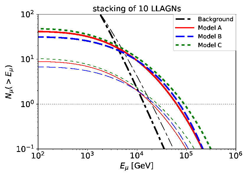
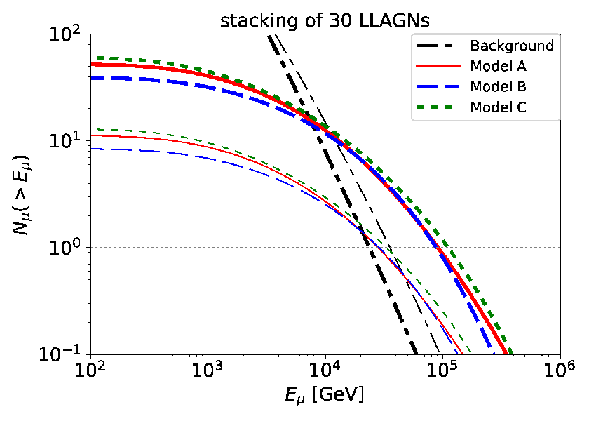
Since the neutrino flux is roughly proportional to the X-ray flux, we place the LLAGNs listed in Ref. Saikia et al. 2018 in order of the X-ray flux, as shown in Table 1, and estimate the number of track events above by stacking them. Figure 6 shows the resulting event number for a 10-year operation with IceCube-Gen2 and IceCube by stacking 10 LLAGNs and 30 LLAGNs. With IceCube-Gen2, we expect 3 – 7 events above 30 TeV where the background is negligible. Interestingly, the neutrinos from the ten brightest LLAGNs will be sufficient for the detection, because stacking more LLAGNs leads to an increase of the atmospheric background. With the current IceCube experiment, the effective area and angular resolution are times smaller and 3 – 5 times larger than those of IceCube-Gen2, respectively. Then, the event number is about 4 – 5 times lower and the background rate is 10 – 30 times higher, making the detection of neutrinos more challenging, as seen in the figures.

V Cascade gamma-ray emission
Hadronuclear and photohadronic processes produce very-high-energy (VHE) gamma rays through neutral pion decay and high-energy electron/positron pairs through charged pion decay and the Bethe-Heitler process. The VHE gamma rays are absorbed by soft photons through the process in the RIAF, and produce additional high-energy electron/positron pairs. The high-energy pairs also emit gamma-rays through synchrotron, inverse Compton scattering, and bremsstrahlung, leading to electromagnetic cascades. We calculate the cascade emission by solving the kinetic equations of photons and electron/positron pairs (see Refs. Murase 2018; Murase et al. 2019b; Murase et al. 2019a):
| (31) |
| (32) |
where is the differential number density ( or ), is the particle source term from the process ( (inverse Compton scattering), ( pair production), syn (synchrotron), or ff (bremsstrahlung)), is the injection term from the hadronic interaction, and is the energy loss rate for the electrons from the process ( (inverse Compton scattering), syn (synchrotron), ff (bremsstrahlung), or Cou (Coulomb collision)). We calculate the cascade spectra using spherical coordinates, while the other calculations are made in cylindrical coordinates. The effect of geometry has little influence on our results.
Here, we approximately treat the injection terms of photons and pairs from hadronic interactions. The injection terms for photons and pairs consist of the sum of the relevant processes: and . We approximate the terms due to Bethe-Heitler and processes to be
| (33) | |||
| (34) | |||
| (35) |
where and for photomeson production, and for Bethe-Heitler process. For the injection terms from interactions, see Ref. Murase et al. 2019b.
We plot proton-induced cascade gamma-ray spectra in Figure 3. A sufficiently developed cascade emission generates a flat spectrum below the critical energy at which attenuation becomes ineffective. The optical depth to the electron-positron pair production is estimated to be
| (36) |
where is the gamma-ray energy, , , and is the Heaviside step function Coppi and Blandford 1990. We tabulate the values of the critical energy, , at which in Table 2. We can see flat spectra below the critical energy. Note that the tabulated values are approximately calculated using a fitting formula, while the cascade calculations are performed with the exact cross section. We overplot the Fermi LAT sensitivity curve in the high galactic latitude region with a 10-year exposure obtained from Ref. De Angelis et al. 2017. The predicted fluxes are lower than the sensitivity curve for all the cases. The Cherenkov Telescope Array (CTA) has a better sensitivity above 30 GeV than LAT, but the cascade gamma-ray flux is considerably suppressed in the VHE range due to the attenuation. For a lower object that has a higher value of , such as NGC 5866, the cascade flux is too low to be detected by CTA. Therefore, it would be challenging to detect the cascade gamma rays with current and near-future instruments, except for Sgr A*.
Sgr A* has two distinct emission phases: the quiescent and flaring states (see Ref. Genzel et al. 2010 for review). The X-ray emission from the quiescent state of Sgr A* is spatially extended to 1”, which corresponds to for a black hole of Baganoff et al. 2003. Hence, our model is not applicable to the quiescent state. On the other hand, the flaring state of Sgr A* shows times higher flux than the quiescent state with the time variability of h Porquet et al. 2003. This variability timescale implies that the emission region should be . However, the value of for the brightest flare estimated by Equation (3) is less than . Since our model is not applicable to such a low-accretion-rate system (see Section II), we avoid discussing it in detail. The detailed estimate should be made in the future (see Ref. Rodríguez-Ramírez et al. 2019 for related discussion).
VI Summary
We have investigated high-energy multi-messenger emissions, including the MeV gamma-rays, high-energy gamma-rays, and neutrinos, from nearby individual LLAGNs, focusing on their multi-messenger detection prospects. We have refined the RIAF model of LLAGNs, referring to recent simulation results. Our one-zone model is roughly consistent with the observed X-ray features, such as an anti-correlation between the Eddington ratio and the spectral index. RIAFs with emit strong MeV gamma rays through Comptonization, which will be detected by the future MeV satellites such as e-ASTROGAM, AMEGO, and GRAMS.
We have also calculated the neutrino and cascade gamma-ray spectra from accelerated protons. We considered three models for the proton spectrum. In model A, we considered stochastic acceleration by turbulence and solve the diffusion equation in momentum space. In models B and C, we do not specify the acceleration mechanism and assumed an injection term with a power-law and an exponential cutoff. Using such proton spectra, we have numerically calculated the neutrino spectra, taking account of the relevant cooling processes and the decay spectra. Since inelastic collisions provide the main channel for high-energy neutrino production, the neutrino spectrum follows the proton spectrum. Close to the cutoff energy, TeV, the photomeson production is as efficient as interactions, leading to a comparable contribution to the neutrino flux. With a few to 10 LLAGNs stacked, a 10-year operation of IceCube-Gen2 will enable us to detect a few to several neutrinos from LLAGNs, otherwise they will put meaningful constraints on the parameter space. On the other hand, the cascade emission is difficult to detect with Fermi or CTA. Bright objects have a lower cutoff energy, while objects with a higher value of the cutoff energy are too dim to produce a detectable signal.
AGN coronae and RIAFs are thought to be promising sites of particle acceleration, and accompanying papers suggest the AGN cores as the main origin of the mysterious 10 – 100 TeV component in the diffuse neutrino flux observed in IceCube Murase et al. 2019a. The model predicts that both Seyfert galaxies and LLAGNs are promising sources of high-energy neutrinos and MeV gamma rays. Our studies suggest the relevance of multi-messenger searches for LLAGNs whether the 10 – 100 TeV neutrinos mainly come from Seyfert galaxies or LLAGNs.
Acknowledgements.
This work is supported in part by JSPS Oversea Research Fellowship, JSPS Postdoctral Fellowship, the IGC postdoctoral fellowship program (S.S.K.), the Alfred P. Sloan Foundation, NSF Grant No. PHY-1620777 (K.M.), and the Eberly Foundation (P.M.).References
- Aartsen et al. (2013) M. G. Aartsen, R. Abbasi, Y. Abdou, M. Ackermann, J. Adams, J. A. Aguilar, M. Ahlers, D. Altmann, J. Auffenberg, X. Bai, and et al., Physical Review Letters 111, 021103 (2013), arXiv:1304.5356 [astro-ph.HE] .
- IceCube Collaboration (2013) IceCube Collaboration, Science 342, 1242856 (2013), arXiv:1311.5238 [astro-ph.HE] .
- Aartsen et al. (2014) M. G. Aartsen, M. Ackermann, J. Adams, J. A. Aguilar, M. Ahlers, M. Ahrens, D. Altmann, T. Anderson, C. Arguelles, T. C. Arlen, and et al., Physical Review Letters 113, 101101 (2014), arXiv:1405.5303 [astro-ph.HE] .
- Aartsen et al. (2015a) M. G. Aartsen, M. Ackermann, J. Adams, J. A. Aguilar, M. Ahlers, M. Ahrens, D. Altmann, T. Anderson, C. Arguelles, T. C. Arlen, and et al., Phys. Rev. D 91, 022001 (2015a), arXiv:1410.1749 [astro-ph.HE] .
- Aartsen et al. (2015b) M. G. Aartsen, K. Abraham, M. Ackermann, J. Adams, J. A. Aguilar, M. Ahlers, M. Ahrens, D. Altmann, T. Anderson, M. Archinger, and et al., ApJ 809, 98 (2015b), arXiv:1507.03991 [astro-ph.HE] .
- Ahlers and Halzen (2017) M. Ahlers and F. Halzen, Progress of Theoretical and Experimental Physics 2017, 12A105 (2017).
- Waxman and Bahcall (1997) E. Waxman and J. Bahcall, Physical Review Letters 78, 2292 (1997), astro-ph/9701231 .
- Mészáros and Waxman (2001) P. Mészáros and E. Waxman, Physical Review Letters 87, 171102 (2001), astro-ph/0103275 .
- Dermer and Atoyan (2003) C. D. Dermer and A. Atoyan, Phys. Rev. Lett. 91, 071102 (2003), arXiv:astro-ph/0301030 [astro-ph] .
- Guetta et al. (2004) D. Guetta, D. Hooper, J. Alvarez-Mun˜Iz, F. Halzen, and E. Reuveni, Astroparticle Physics 20, 429 (2004), astro-ph/0302524 .
- Murase and Nagataki (2006a) K. Murase and S. Nagataki, Phys. Rev. D 73, 063002 (2006a), astro-ph/0512275 .
- Aartsen et al. (2016) M. G. Aartsen, K. Abraham, M. Ackermann, J. Adams, J. A. Aguilar, M. Ahlers, M. Ahrens, D. Altmann, T. Anderson, I. Ansseau, and et al., ApJ 824, 115 (2016), arXiv:1601.06484 [astro-ph.HE] .
- Aartsen et al. (2017) M. G. Aartsen, M. Ackermann, J. Adams, J. A. Aguilar, M. Ahlers, M. Ahrens, I. A. Samarai, D. Altmann, K. Andeen, T. Anderson, and et al., ApJ 843, 112 (2017), arXiv:1702.06868 [astro-ph.HE] .
- Waxman and Bahcall (2000) E. Waxman and J. N. Bahcall, ApJ 541, 707 (2000), hep-ph/9909286 .
- Murase and Nagataki (2006b) K. Murase and S. Nagataki, Physical Review Letters 97, 051101 (2006b), astro-ph/0604437 .
- Murase (2007) K. Murase, Phys. Rev. D 76, 123001 (2007), arXiv:0707.1140 .
- Kimura et al. (2017) S. S. Kimura, K. Murase, P. Mészáros, and K. Kiuchi, ApJ 848, L4 (2017), arXiv:1708.07075 [astro-ph.HE] .
- Murase et al. (2006) K. Murase, K. Ioka, S. Nagataki, and T. Nakamura, ApJ 651, L5 (2006), astro-ph/0607104 .
- Senno et al. (2016) N. Senno, K. Murase, and P. Mészáros, Phys. Rev. D 93, 083003 (2016), arXiv:1512.08513 [astro-ph.HE] .
- Zhang et al. (2018) B. T. Zhang, K. Murase, S. S. Kimura, S. Horiuchi, and P. Mészáros, Phys. Rev. D 97, 083010 (2018), arXiv:1712.09984 [astro-ph.HE] .
- Boncioli et al. (2019) D. Boncioli, D. Biehl, and W. Winter, ApJ 872, 110 (2019), arXiv:1808.07481 [astro-ph.HE] .
- Zhang and Murase (2018) B. T. Zhang and K. Murase, arXiv e-prints , arXiv:1812.10289 (2018), arXiv:1812.10289 [astro-ph.HE] .
- Razzaque et al. (2003) S. Razzaque, P. Mészáros, and E. Waxman, Phys. Rev. D 68, 083001 (2003), arXiv:astro-ph/0303505 [astro-ph] .
- Ando and Beacom (2005) S. Ando and J. F. Beacom, Phys. Rev. Lett. 95, 061103 (2005), arXiv:astro-ph/0502521 [astro-ph] .
- Horiuchi and Ando (2008) S. Horiuchi and S. Ando, Phys. Rev. D 77, 063007 (2008), arXiv:0711.2580 .
- Murase and Ioka (2013) K. Murase and K. Ioka, Physical Review Letters 111, 121102 (2013), arXiv:1306.2274 [astro-ph.HE] .
- He et al. (2018) H.-N. He, A. Kusenko, S. Nagataki, Y.-Z. Fan, and D.-M. Wei, ApJ 856, 119 (2018), arXiv:1803.07478 [astro-ph.HE] .
- Denton and Tamborra (2018) P. B. Denton and I. Tamborra, ApJ 855, 37 (2018), arXiv:1711.00470 [astro-ph.HE] .
- Kimura et al. (2018) S. S. Kimura, K. Murase, I. Bartos, K. Ioka, I. S. Heng, and P. Mészáros, Phys. Rev. D 98, 043020 (2018), arXiv:1805.11613 [astro-ph.HE] .
- Mannheim et al. (1992) K. Mannheim, T. Stanev, and P. L. Biermann, A&A 260, L1 (1992).
- Halzen and Zas (1997) F. Halzen and E. Zas, ApJ 488, 669 (1997), arXiv:astro-ph/9702193 [astro-ph] .
- Atoyan and Dermer (2001) A. Atoyan and C. D. Dermer, Physical Review Letters 87, 221102 (2001), astro-ph/0108053 .
- IceCube-Collaboration et al. (2018) IceCube-Collaboration, Fermi-LAT, MAGIC, AGILE, ASAS-SN, HAWC, H.E.S.S, INTEGRAL, Kanata, Kiso, Kapteyn, L. Telescope, Subaru, Swift/NuSTAR, VERITAS, V.-. teams, et al. (IceCube Collaboration), Science 361, 146 (2018), arXiv:1807.xxxxx [astro-ph.HE] .
- Aartsen et al. (2017a) M. G. Aartsen et al. (IceCube), Astropart. Phys. 92, 30 (2017a), arXiv:1612.06028 [astro-ph.HE] .
- Keivani et al. (2018) A. Keivani, K. Murase, M. Petropoulou, D. B. Fox, S. B. Cenko, S. Chaty, A. Coleiro, J. J. DeLaunay, S. Dimitrakoudis, P. A. Evans, J. A. Kennea, F. E. Marshall, A. Mastichiadis, J. P. Osborne, M. Santand er, A. Tohuvavohu, and C. F. Turley, ApJ 864, 84 (2018), arXiv:1807.04537 [astro-ph.HE] .
- Murase et al. (2018) K. Murase, F. Oikonomou, and M. Petropoulou, ApJ 865, 124 (2018), arXiv:1807.04748 [astro-ph.HE] .
- Liu et al. (2018) R.-Y. Liu, K. Wang, R. Xue, A. M. Taylor, X.-Y. Wang, Z. Li, and H. Yan, arXiv e-prints , arXiv:1807.05113 (2018), arXiv:1807.05113 [astro-ph.HE] .
- Cerruti et al. (2019) M. Cerruti, A. Zech, C. Boisson, G. Emery, S. Inoue, and J. P. Lenain, MNRAS 483, L12 (2019), arXiv:1807.04335 [astro-ph.HE] .
- Gao et al. (2019) S. Gao, A. Fedynitch, W. Winter, and M. Pohl, Nature Astronomy 3, 88 (2019), arXiv:1807.04275 [astro-ph.HE] .
- IceCube-Collaboration (2018) IceCube-Collaboration (IceCube Collaboration), Science 361, 147 (2018), arXiv:1807.xxxxx [astro-ph.HE] .
- Garrappa et al. (2019) S. Garrappa et al. (Fermi-LAT, ASAS-SN, IceCube), (2019), arXiv:1901.10806 [astro-ph.HE] .
- Reimer et al. (2018) A. Reimer, M. Boettcher, and S. Buson, arXiv e-prints , arXiv:1812.05654 (2018), arXiv:1812.05654 [astro-ph.HE] .
- Rodrigues et al. (2018) X. Rodrigues, S. Gao, A. Fedynitch, A. Palladino, and W. Winter, arXiv e-prints , arXiv:1812.05939 (2018), arXiv:1812.05939 [astro-ph.HE] .
- Wang et al. (2018) K. Wang, R.-Y. Liu, Z. Li, X.-Y. Wang, and Z.-G. Dai, arXiv e-prints , arXiv:1809.00601 (2018), arXiv:1809.00601 [astro-ph.HE] .
- Aartsen et al. (2017b) M. G. Aartsen et al. (IceCube), Astrophys. J. 835, 45 (2017b), arXiv:1611.03874 [astro-ph.HE] .
- Neronov et al. (2017) A. Neronov, D. V. Semikoz, and K. Ptitsyna, Astron. Astrophys. 603, A135 (2017), arXiv:1611.06338 [astro-ph.HE] .
- Yuan et al. (2019) C. Yuan, K. Murase, and P. Mészáros, arXiv e-prints , arXiv:1904.06371 (2019), arXiv:1904.06371 [astro-ph.HE] .
- Hooper et al. (2019) D. Hooper, T. Linden, and A. Vieregg, J. Cosmology Astropart. Phys 2019, 012 (2019), arXiv:1810.02823 [astro-ph.HE] .
- Murase and Waxman (2016) K. Murase and E. Waxman, Phys. Rev. D94, 103006 (2016), arXiv:1607.01601 [astro-ph.HE] .
- Ackermann et al. (2015) M. Ackermann et al. (Fermi-LAT), Astrophys. J. 799, 86 (2015), arXiv:1410.3696 [astro-ph.HE] .
- Murase et al. (2013) K. Murase, M. Ahlers, and B. C. Lacki, Phys. Rev. D 88, 121301 (2013), arXiv:1306.3417 [astro-ph.HE] .
- Aartsen et al. (2015) M. G. Aartsen et al. (IceCube), Phys. Rev. Lett. 115, 081102 (2015), arXiv:1507.04005 [astro-ph.HE] .
- Aartsen et al. (2017c) M. G. Aartsen et al. (IceCube Collaboration), (2017c), arXiv:1710.01179 [astro-ph.HE] .
- Palladino and Winter (2018) A. Palladino and W. Winter, A&A 615, A168 (2018), arXiv:1801.07277 [astro-ph.HE] .
- Murase et al. (2016) K. Murase, D. Guetta, and M. Ahlers, Phys. Rev. Lett. 116, 071101 (2016), arXiv:1509.00805 [astro-ph.HE] .
- Loeb and Waxman (2006) A. Loeb and E. Waxman, J. Cosmology Astropart. Phys 5, 003 (2006), astro-ph/0601695 .
- He et al. (2013) H.-N. He, T. Wang, Y.-Z. Fan, S.-M. Liu, and D.-M. Wei, Phys. Rev. D 87, 063011 (2013), arXiv:1303.1253 [astro-ph.HE] .
- Anchordoqui et al. (2014) L. A. Anchordoqui, T. C. Paul, L. H. M. da Silva, D. F. Torres, and B. J. Vlcek, Phys. Rev. D 89, 127304 (2014), arXiv:1405.7648 [astro-ph.HE] .
- Liu et al. (2014) R.-Y. Liu, X.-Y. Wang, S. Inoue, R. Crocker, and F. Aharonian, Phys. Rev. D 89, 083004 (2014), arXiv:1310.1263 [astro-ph.HE] .
- Tamborra et al. (2014) I. Tamborra, S. Ando, and K. Murase, J. Cosmology Astropart. Phys 9, 043 (2014), arXiv:1404.1189 [astro-ph.HE] .
- Senno et al. (2015) N. Senno, P. Mészáros, K. Murase, P. Baerwald, and M. J. Rees, ArXiv e-prints (2015), arXiv:1501.04934 [astro-ph.HE] .
- Xiao et al. (2016) D. Xiao, P. Mészáros, K. Murase, and Z.-G. Dai, ApJ 826, 133 (2016), arXiv:1604.08131 [astro-ph.HE] .
- Bechtol et al. (2017) K. Bechtol, M. Ahlers, M. Di Mauro, M. Ajello, and J. Vandenbroucke, ApJ 836, 47 (2017), arXiv:1511.00688 [astro-ph.HE] .
- Sudoh et al. (2018) T. Sudoh, T. Totani, and N. Kawanaka, Publications of the Astronomical Society of Japan 70, 49 (2018), arXiv:1801.09683 [astro-ph.HE] .
- Murase et al. (2008) K. Murase, S. Inoue, and S. Nagataki, ApJ 689, L105 (2008), arXiv:0805.0104 .
- Kotera et al. (2009) K. Kotera, D. Allard, K. Murase, J. Aoi, Y. Dubois, T. Pierog, and S. Nagataki, ApJ 707, 370 (2009), arXiv:0907.2433 [astro-ph.HE] .
- Zandanel et al. (2015) F. Zandanel, I. Tamborra, S. Gabici, and S. Ando, A&A 578, A32 (2015), arXiv:1410.8697 [astro-ph.HE] .
- Fang and Olinto (2016) K. Fang and A. V. Olinto, ApJ 828, 37 (2016), arXiv:1607.00380 [astro-ph.HE] .
- Fang and Murase (2018) K. Fang and K. Murase, Nature Physics 14, 396 (2018), arXiv:1704.00015 [astro-ph.HE] .
- Becker Tjus et al. (2014) J. Becker Tjus, B. Eichmann, F. Halzen, A. Kheirandish, and S. M. Saba, Phys. Rev. D 89, 123005 (2014), arXiv:1406.0506 [astro-ph.HE] .
- Hooper (2016) D. Hooper, Journal of Cosmology and Astro-Particle Physics 2016, 002 (2016), arXiv:1605.06504 [astro-ph.HE] .
- Berezinskii and Ginzburg (1981) V. S. Berezinskii and V. L. Ginzburg, MNRAS 194, 3 (1981).
- Kazanas and Ellison (1986) D. Kazanas and D. C. Ellison, ApJ 304, 178 (1986).
- Zdziarski (1986) A. A. Zdziarski, ApJ 305, 45 (1986).
- Begelman et al. (1990) M. C. Begelman, B. Rudak, and M. Sikora, ApJ 362, 38 (1990).
- Stecker et al. (1991) F. W. Stecker, C. Done, M. H. Salamon, and P. Sommers, Physical Review Letters 66, 2697 (1991).
- Bednarek and Protheroe (1999) W. Bednarek and R. J. Protheroe, MNRAS 302, 373 (1999), arXiv:astro-ph/9802288 [astro-ph] .
- Alvarez-Muñiz and Mészáros (2004) J. Alvarez-Muñiz and P. Mészáros, Phys. Rev. D 70, 123001 (2004), astro-ph/0409034 .
- Shakura and Sunyaev (1973) N. I. Shakura and R. A. Sunyaev, A&A 24, 337 (1973).
- Malkan (1983) M. A. Malkan, ApJ 268, 582 (1983).
- Czerny and Elvis (1987) B. Czerny and M. Elvis, ApJ 321, 305 (1987).
- Marconi et al. (2004) A. Marconi, G. Risaliti, R. Gilli, L. K. Hunt, R. Maiolino, and M. Salvati, MNRAS 351, 169 (2004), astro-ph/0311619 .
- Hopkins et al. (2007) P. F. Hopkins, G. T. Richards, and L. Hernquist, ApJ 654, 731 (2007), arXiv:astro-ph/0605678 [astro-ph] .
- Lusso et al. (2012) E. Lusso, A. Comastri, B. D. Simmons, M. Mignoli, G. Zamorani, C. Vignali, M. Brusa, F. Shankar, D. Lutz, J. R. Trump, R. Maiolino, R. Gilli, M. Bolzonella, S. Puccetti, M. Salvato, C. D. Impey, F. Civano, M. Elvis, V. Mainieri, J. D. Silverman, A. M. Koekemoer, A. Bongiorno, A. Merloni, S. Berta, E. Le Floc’h, B. Magnelli, F. Pozzi, and L. Riguccini, MNRAS 425, 623 (2012), arXiv:1206.2642 [astro-ph.CO] .
- Kalashev et al. (2015) O. Kalashev, D. Semikoz, and I. Tkachev, Soviet Journal of Experimental and Theoretical Physics 120, 541 (2015), arXiv:1410.8124 [astro-ph.HE] .
- Inoue et al. (2019) Y. Inoue, D. Khangulyan, S. Inoue, and A. Doi, arXiv e-prints , arXiv:1904.00554 (2019), arXiv:1904.00554 [astro-ph.HE] .
- Murase et al. (2019a) K. Murase, S. S. Kimura, and P. Meszaros, arXiv e-prints , arXiv:1904.04226 (2019a), arXiv:1904.04226 [astro-ph.HE] .
- Ho (2008) L. C. Ho, ARA&A 46, 475 (2008), arXiv:0803.2268 .
- Narayan and Yi (1994) R. Narayan and I. Yi, ApJ 428, L13 (1994), astro-ph/9403052 .
- Yuan and Narayan (2014) F. Yuan and R. Narayan, ARA&A 52, 529 (2014), arXiv:1401.0586 [astro-ph.HE] .
- Kimura et al. (2015) S. S. Kimura, K. Murase, and K. Toma, ApJ 806, 159 (2015), arXiv:1411.3588 [astro-ph.HE] .
- Khiali and de Gouveia Dal Pino (2016) B. Khiali and E. M. de Gouveia Dal Pino, MNRAS 455, 838 (2016), arXiv:1506.01063 [astro-ph.HE] .
- Righi et al. (2019) C. Righi, F. Tavecchio, and S. Inoue, MNRAS 483, L127 (2019), arXiv:1807.10506 [astro-ph.HE] .
- Machida and Matsumoto (2003) M. Machida and R. Matsumoto, ApJ 585, 429 (2003), astro-ph/0211240 .
- McKinney (2006) J. C. McKinney, MNRAS 368, 1561 (2006), astro-ph/0603045 .
- Ohsuga and Mineshige (2011) K. Ohsuga and S. Mineshige, ApJ 736, 2 (2011), arXiv:1105.5474 [astro-ph.HE] .
- Narayan et al. (2012) R. Narayan, A. SÄ dowski, R. F. Penna, and A. K. Kulkarni, MNRAS 426, 3241 (2012), arXiv:1206.1213 [astro-ph.HE] .
- Penna et al. (2013) R. F. Penna, A. Sadowski, A. K. Kulkarni, and R. Narayan, MNRAS 428, 2255 (2013), arXiv:1211.0526 [astro-ph.HE] .
- Kimura et al. (2019) S. S. Kimura, K. Tomida, and K. Murase, MNRAS 485, 163 (2019), arXiv:1812.03901 [astro-ph.HE] .
- Ressler et al. (2017) S. M. Ressler, A. Tchekhovskoy, E. Quataert, and C. F. Gammie, MNRAS 467, 3604 (2017), arXiv:1611.09365 [astro-ph.HE] .
- Chael et al. (2018) A. Chael, M. Rowan, R. Narayan, M. Johnson, and L. Sironi, MNRAS 478, 5209 (2018), arXiv:1804.06416 [astro-ph.HE] .
- Ball et al. (2018) D. Ball, L. Sironi, and F. Özel, ApJ 862, 80 (2018), arXiv:1803.05556 [astro-ph.HE] .
- Martin et al. (2019) R. G. Martin, C. J. Nixon, J. E. Pringle, and M. Livio, arXiv e-prints , arXiv:1901.01580 (2019), arXiv:1901.01580 [astro-ph.HE] .
- Xie and Yuan (2012) F.-G. Xie and F. Yuan, MNRAS 427, 1580 (2012), arXiv:1207.3113 [astro-ph.HE] .
- Mahadevan and Quataert (1997) R. Mahadevan and E. Quataert, ApJ 490, 605 (1997), astro-ph/9705067 .
- Kato et al. (2008) S. Kato, J. Fukue, and S. Mineshige, Black-Hole Accretion Disks — Towards a New Paradigm —, 549 pages, including 12 Chapters, 9 Appendices, ISBN 978-4-87698-740-5, Kyoto University Press (Kyoto, Japan), 2008. (Kyoto University Press, 2008).
- Narayan and Yi (1995) R. Narayan and I. Yi, ApJ 452, 710 (1995), astro-ph/9411059 .
- Abramowicz et al. (1995) M. A. Abramowicz, X. Chen, S. Kato, J.-P. Lasota, and O. Regev, ApJ 438, L37 (1995), astro-ph/9409018 .
- Mahadevan (1997) R. Mahadevan, ApJ 477, 585 (1997), astro-ph/9609107 .
- Quataert and Gruzinov (1999) E. Quataert and A. Gruzinov, ApJ 520, 248 (1999), astro-ph/9803112 .
- Sharma et al. (2007) P. Sharma, E. Quataert, G. W. Hammett, and J. M. Stone, ApJ 667, 714 (2007), astro-ph/0703572 .
- Riquelme et al. (2012) M. A. Riquelme, E. Quataert, P. Sharma, and A. Spitkovsky, ApJ 755, 50 (2012), arXiv:1201.6407 [astro-ph.HE] .
- Kunz et al. (2014) M. W. Kunz, A. A. Schekochihin, and J. M. Stone, Physical Review Letters 112, 205003 (2014), arXiv:1402.0010 [astro-ph.HE] .
- Hoshino (2013) M. Hoshino, ApJ 773, 118 (2013), arXiv:1306.6720 [astro-ph.HE] .
- Hoshino (2015) M. Hoshino, Physical Review Letters 114, 061101 (2015), arXiv:1502.02452 [astro-ph.HE] .
- Sironi and Narayan (2015) L. Sironi and R. Narayan, ApJ 800, 88 (2015), arXiv:1411.5685 [astro-ph.HE] .
- Sironi (2015) L. Sironi, ApJ 800, 89 (2015), arXiv:1411.6014 [astro-ph.HE] .
- Zhdankin et al. (2018) V. Zhdankin, D. A. Uzdensky, G. R. Werner, and M. C. Begelman, arXiv e-prints , arXiv:1809.01966 (2018), arXiv:1809.01966 [astro-ph.HE] .
- Wang et al. (2004) J.-M. Wang, K.-Y. Watarai, and S. Mineshige, ApJ 607, L107 (2004), arXiv:astro-ph/0407160 [astro-ph] .
- Liu et al. (2016) Z. Liu, A. Merloni, A. Georgakakis, M.-L. Menzel, J. Buchner, K. Nandra, M. Salvato, Y. Shen, M. Brusa, and A. Streblyanska, MNRAS 459, 1602 (2016), arXiv:1605.00207 [astro-ph.HE] .
- Saikia et al. (2018) P. Saikia, E. Körding, D. L. Coppejans, H. Falcke, D. Williams, R. D. Baldi, I. Mchardy, and R. Beswick, A&A 616, A152 (2018), arXiv:1805.06696 [astro-ph.HE] .
- Eracleous et al. (2010) M. Eracleous, J. A. Hwang, and H. M. L. G. Flohic, ApJS 187, 135 (2010), arXiv:1001.2924 [astro-ph.GA] .
- Gu and Cao (2009) M. Gu and X. Cao, MNRAS 399, 349 (2009), arXiv:0906.3560 [astro-ph.GA] .
- She et al. (2018) R. She, L. C. Ho, H. Feng, and C. Cui, ApJ 859, 152 (2018), arXiv:1804.07482 [astro-ph.HE] .
- Younes et al. (2019) G. Younes, A. Ptak, L. C. Ho, F.-G. Xie, Y. Terasima, F. Yuan, D. Huppenkothen, and M. Yukita, ApJ 870, 73 (2019), arXiv:1811.10657 [astro-ph.GA] .
- De Angelis et al. (2017) A. De Angelis, V. Tatischeff, M. Tavani, U. Oberlack, I. Grenier, L. Hanlon, R. Walter, A. Argan, P. von Ballmoos, and A. Bulgarelli, Experimental Astronomy 44, 25 (2017), arXiv:1611.02232 [astro-ph.HE] .
- Moiseev and Amego Team (2017) A. Moiseev and Amego Team, International Cosmic Ray Conference 301, 798 (2017).
- Aramaki et al. (2020) T. Aramaki, P. O. H. Adrian, G. Karagiorgi, and H. Odaka, Astroparticle Physics 114, 107 (2020), arXiv:1901.03430 [astro-ph.HE] .
- Zenitani and Hoshino (2001) S. Zenitani and M. Hoshino, ApJ 562, L63 (2001), arXiv:1402.7139 [astro-ph.HE] .
- Kowal et al. (2012) G. Kowal, E. M. de Gouveia Dal Pino, and A. Lazarian, Physical Review Letters 108, 241102 (2012), arXiv:1202.5256 [astro-ph.HE] .
- Sironi and Spitkovsky (2014) L. Sironi and A. Spitkovsky, ApJ 783, L21 (2014), arXiv:1401.5471 [astro-ph.HE] .
- Kunz et al. (2016) M. W. Kunz, J. M. Stone, and E. Quataert, Physical Review Letters 117, 235101 (2016), arXiv:1608.07911 [astro-ph.HE] .
- Kimura et al. (2016) S. S. Kimura, K. Toma, T. K. Suzuki, and S.-i. Inutsuka, ApJ 822, 88 (2016), arXiv:1602.07773 [astro-ph.HE] .
- Comisso and Sironi (2018) L. Comisso and L. Sironi, Phys. Rev. Lett. 121, 255101 (2018), arXiv:1809.01168 [astro-ph.HE] .
- Wong et al. (2019) K. Wong, V. Zhdankin, D. A. Uzdensky, G. R. Werner, and M. C. Begelman, arXiv e-prints , arXiv:1901.03439 (2019), arXiv:1901.03439 [astro-ph.HE] .
- Chen et al. (2018) A. Y. Chen, Y. Yuan, and H. Yang, ApJ 863, L31 (2018), arXiv:1805.11039 [astro-ph.HE] .
- Levinson and Cerutti (2018) A. Levinson and B. Cerutti, A&A 616, A184 (2018), arXiv:1803.04427 [astro-ph.HE] .
- Takahara and Kusunose (1985) F. Takahara and M. Kusunose, Progress of Theoretical Physics 73, 1390 (1985).
- Kimura et al. (2014) S. S. Kimura, K. Toma, and F. Takahara, ApJ 791, 100 (2014), arXiv:1407.0115 [astro-ph.HE] .
- Pringle (1981) J. E. Pringle, ARA&A 19, 137 (1981).
- Abramowicz et al. (1988) M. A. Abramowicz, B. Czerny, J. P. Lasota, and E. Szuszkiewicz, ApJ 332, 646 (1988).
- Blandford and Eichler (1987) R. Blandford and D. Eichler, Phys. Rep. 154, 1 (1987).
- Petrosian (2012) V. Petrosian, Space Sci. Rev. 173, 535 (2012), arXiv:1205.2136 [astro-ph.HE] .
- Dermer et al. (1996) C. D. Dermer, J. A. Miller, and H. Li, ApJ 456, 106 (1996), astro-ph/9508069 .
- Stawarz and Petrosian (2008) Ł. Stawarz and V. Petrosian, ApJ 681, 1725 (2008), arXiv:0803.0989 .
- Kakuwa (2016) J. Kakuwa, ApJ 816, 24 (2016), arXiv:1511.07738 [astro-ph.HE] .
- Chang and Cooper (1970) J. S. Chang and G. Cooper, Journal of Computational Physics 6, 1 (1970).
- Park and Petrosian (1996) B. T. Park and V. Petrosian, The Astrophysical Journal Supplement Series 103, 255 (1996).
- Dermer and Menon (2009) C. D. Dermer and G. Menon, High Energy Radiation from Black Holes: Gamma Rays, Cosmic Rays, and Neutrinos (2009).
- Giacalone and Jokipii (1999) J. Giacalone and J. R. Jokipii, ApJ 520, 204 (1999).
- Casse et al. (2002) F. Casse, M. Lemoine, and G. Pelletier, Phys. Rev. D 65, 023002 (2002), astro-ph/0109223 .
- Kafexhiu et al. (2014) E. Kafexhiu, F. Aharonian, A. M. Taylor, and G. S. Vila, Phys. Rev. D 90, 123014 (2014), arXiv:1406.7369 [astro-ph.HE] .
- Stepney and Guilbert (1983) S. Stepney and P. W. Guilbert, MNRAS 204, 1269 (1983).
- Chodorowski et al. (1992) M. J. Chodorowski, A. A. Zdziarski, and M. Sikora, ApJ 400, 181 (1992).
- Becker et al. (2006) P. A. Becker, T. Le, and C. D. Dermer, ApJ 647, 539 (2006), astro-ph/0604504 .
- Kelner et al. (2006) S. R. Kelner, F. A. Aharonian, and V. V. Bugayov, Phys. Rev. D 74, 034018 (2006), astro-ph/0606058 .
- Laha et al. (2013) R. Laha, J. F. Beacom, B. Dasgupta, S. Horiuchi, and K. Murase, Phys. Rev. D88, 043009 (2013), arXiv:1306.2309 [astro-ph.HE] .
- Aartsen et al. (2014) M. G. Aartsen et al. (IceCube), Astrophys. J. 796, 109 (2014), arXiv:1406.6757 [astro-ph.HE] .
- Murase (2018) K. Murase, Phys. Rev. D 97, 081301 (2018), arXiv:1705.04750 [astro-ph.HE] .
- Murase et al. (2019b) K. Murase, A. Franckowiak, K. Maeda, R. Margutti, and J. F. Beacom, ApJ 874, 80 (2019b), arXiv:1807.01460 [astro-ph.HE] .
- Coppi and Blandford (1990) P. S. Coppi and R. D. Blandford, MNRAS 245, 453 (1990).
- Genzel et al. (2010) R. Genzel, F. Eisenhauer, and S. Gillessen, Reviews of Modern Physics 82, 3121 (2010), arXiv:1006.0064 [astro-ph.GA] .
- Baganoff et al. (2003) F. K. Baganoff, Y. Maeda, M. Morris, M. W. Bautz, W. N. Brandt, W. Cui, J. P. Doty, E. D. Feigelson, G. P. Garmire, S. H. Pravdo, G. R. Ricker, and L. K. Townsley, ApJ 591, 891 (2003), arXiv:astro-ph/0102151 [astro-ph] .
- Porquet et al. (2003) D. Porquet, P. Predehl, B. Aschenbach, N. Grosso, A. Goldwurm, P. Goldoni, R. S. Warwick, and A. Decourchelle, A&A 407, L17 (2003), arXiv:astro-ph/0307110 [astro-ph] .
- Rodríguez-Ramírez et al. (2019) J. C. Rodríguez-Ramírez, E. M. de Gouveia Dal Pino, and R. Alves Batista, ApJ 879, 6 (2019), arXiv:1904.05765 [astro-ph.HE] .