Modelling physical limits of migration by a kinetic model with non-local sensing

During their motion, cells sense the external environment thanks to their protrusions which may extend up to several cell diameters. The captured chemical or mechanical signals activate transduction pathways inside the cell leading to the cell response which consists in $(i)$ the formation of a “head” and a “tail”, $(ii)$ in the triggering of actin polimerization at the front edge and depolarization at the rear of the cell, and $(iii)$ in the activation of adhesion molecules and traction forces leading eventually to motion (Abercrombie and Heaysman, 1953; Adler, 1966; Block et al., 1983). The above steps can be somewhat distinguished in polarization and mobility mechanisms. For instance, Devreotes and Janetopoulos, 2003 showed that D. Discoideum cells polarize in response to cAMP even when treated with inhibitors of the cytoskeleton, such as latrunculin A, that inhibit cell motion.

After external stimuli determine the preferential direction of a cell, in addition to internal causes, other environmental cues may promote or hamper the movement in that direction, such as the cell density. For instance, the presence of other cells influences cell migration in a two-fold way. On one hand cells may be attracted due to the mutual interaction of transmembrane adhesion molecules (${\it e.g.}$, cadherin complexes). On the other hand, cells may stay away from too crowded regions or just lean on their boundaries. Another important migration determinant is the extra-cellular matrix (ECM), ${\it i.e.}$ the network of macro-molecules (such as proteoglycans, collagene, fibronectin, and elastin) representing one of the main non-cellular component of all tissues and organs. In fact, it provides cells with a physical scaffold. Its density, stiffness, and microstructure highly influence the behaviour of cells and in particular their migration mode (te Boekhorst et al., 2016). Again, the presence of ECM is necessary to form focal adhesion sites through the activation of integrins that are used by the cell to exert traction forces, but if it is too dense it might represent a steric obstacle to cell motion.

In particular, experiments (see, for instance, Schoumacher et al., 2010; Shankar et al., 2010) show that while the cytoplasm is very flexible and able to accommodate nearly any pore size (including $1\mu m^{2}$ gaps in collagen gels and $0.8\mu m^{2}$ pores of polycarbonate membranes), the cell nucleus is five- to ten-fold stiffer than the surrounding cytoplasm and, with a typical diameter of $3-10\mu m$, might be larger than the ECM fiber spacing (Davidson et al., 2014). During MMP-independent migration (${\it i.e.}$, when the proteolytic machinery is inhibited) and in spite of cell cytoplasm protrusions into the ECM trying to pull the nucleus inside, the stiff nucleus may be unable to squeeze through narrow pores, setting a critical pore size below which MMP-inhibited cells remain trapped (Wolf et al., 2013). This phenomenon is named physical limit of migration and it has been recently studied from the modelling point of view by Scianna et al., 2013; Scianna and Preziosi, 2013; Scianna and Preziosi, 2014 using cellular Potts models and by Arduino and Preziosi, 2015; Giverso et al., 2014; Giverso et al., 2017 using continuum mechanics methods.

The aim of this article is to include such effects extending the kinetic model developed by Loy and Preziosi, 2019, where possibly independent cues are sensed by cells in a non-local way and used to determine respectively cell polarization and speed. The transport kinetic equation implements then a velocity jump process that describes the movement performed by the cell as an alternation of runs over straight lines and re-orientations (also called tumbles or turnings) (Stroock, 1974), also considering the bias induced by external stimuli, as done by Alt, 1980 and Othmer et al., 1988. Such an equation describes the evolution of a single-particle density distribution like in the Boltzmann equation (Cercignani, 1987). The main elements of the velocity-jump process are the tumbling frequency, the mean speed, and the transition (also called turning or tumbling) probability that describes the probability of choosing a certain velocity after re-orientation. The mean speed, mean runtime (which is the inverse of the frequency), and the tumbling probability may be measured from individual patterns of members of the population.

In the literature many models considered different sensing strategies and their relation to the determination of cell re-orientation and speed. Focusing on non-local aspects, tipically in position jump processes the transition probabilities depend on the acquisition of information sensed at a certain location (${\it e.g.}$ at the target or at the present location) or by averaging the signal over a certain neighborhood as done by Othmer and Stevens, 2001 and by Painter and Sherratt, 2003.

In general, a way of including cell sensing is to consider a non-local average of the external fields. Othmer and Hillen, 2002 and Hillen et al., 2007 introduced a finite sensing radius and defined a non-local gradient as the average of the external field on a surface which represents the membrane of the cell. This idea was also used for cell adhesion and haptotaxis by Armstrong et al., 2006 yielding a macroscopic integro-differential equation. Buttenschön et al., 2018 recently derived this type of models from a space jump process. Other macroscopic models describing cell migration with non-local measures of the environment were proposed by Painter et al., 2010; Painter et al., 2015; Painter and Hillen, 2002. Schmeiser and Nouri, 2017 considered a kinetic model with velocity jumps biased towards the chemical concentration gradient. Similar equations were also proposed in 2D set-ups by Colombi et al., 2015; Colombi et al., 2017, and applied to model crowd dynamics and traffic flow for instance by Tosin and Frasca, 2011. Eftimie, 2012 and Carrillo et al., 2015 also proposed a non-local kinetic models including repulsion, alignement and attraction and used it for modelling tumor dynamics (Eftimie et al., 2017) and cell polarisation in heterogeneous cancer cell populations (Bitsouni and Eftimie, 2018).

In Loy and Preziosi, 2019 the transition probability of the transport equation models the probability of choosing a certain velocity direction and speed according to an environmental sensing over a finite neighbourhood of the cell, giving the kinetic model a non-local character. In particular, a double bias is considered, as cells perform a double sensing both of a tactic cue influencing the probability of polarizing in a certain direction and of an environmental cue, usually of mechanical origins, affecting its speed in the polarization direction. For instance, in presence of a chemoattractant giving a preferential direction of motion, a volume filling effect can hamper the motion in a certain direction due to cell overcrowding.

In the present work, then, the focus is on how to include in kinetic models the effect of physical limits of migration. These include the dependence of the sensing radius on physical characteristics of the environment or on the omotypic or heterotypic cell distributions, that might even hamper the real possibility of cells of measuring in a certain region. In particular, this means that the interval with valuable information to determine cell motion, depends on space, time and direction of sensing. We also discuss how limiting the sampling volume determines the type of macroscopic limit that can be performed.

With this aim in mind, the plan of the article is then the following. In Section 2 the kinetic modelling framework is introduced and then specialised to the case of physical limits of migration in Section 3. In particular, the concept of limitation of sensing radius and its effect on motility is qualitatively described. Section 4 focuses on deducing the appropriated macroscopic limit of the kinetic model showing that in presence of physical limits of migration the macroscopic speed does not vanish in general and therefore the appropriate limit is hyperbolic. Section 5 starts analysing the model from a simpler case in which there is no cue determining a preferred polarization in space, ${\it e.g.}$, no chemotaxis, but only mechanical cues influencing cell speed. Simulations of the kinetic model are performed focusing on volume filling effects in Section 5.1 and on cell-ECM interactions in Section 5.2. A particular attention is paid to pointing out what is the effect of different modelling assumptions and how some choices might lead to non-physical results. Then, in Section 6 chemotaxis and cell-cell adhesion are added as mechanisms influencing cell polarization in order to consider the simultaneous presence of physical limits of migration and cell polarization. A final section draws some conclusions pointing out to other open issues.

Let us describe the cell population through the distribution density $p=p(t,{\bf x},v,\hat{\bf v})$ parametrized by the time $t>0$, the position ${\bf x}\in\Omega\subseteq\mathbb{R}^{d}$, the speed $v\in[0,U]$, where $U$ is the maximal speed a cell can achieve, and the polarization direction $\hat{\bf v}\in\mathbb{S}^{d-1}$ where $\mathbb{S}^{d-1}$ is the unit sphere boundary in $\mathbb{R}^{d}$. The choice of representing the distribution function $p$ depending on velocity modulus and direction, instead of the velocity vector ${\bf v}=v\hat{\bf v}$, lies in the need of separating the mechanisms governing cell polarization and motility, for instance in response of chemotaxis and in presence of other factors, typically of mechanical origins, influencing cell speed.

The mesoscopic model consists in the transport equation for the cell distribution

$$\dfrac{\partial p}{\partial t}(t,{\bf x},v,\hat{\bf v})+{\bf v}\cdot\nabla p(t,{\bf x},v,\hat{\bf v})=\mathcal{J}[p](t,{\bf x},v,\hat{\bf v})$$

(1)

where the operator $\nabla$ denotes the spatial gradient. The term $\mathcal{J}[p](t,{\bf x},v,\hat{\bf v})$, named turning operator, is an integral operator that describes the change in velocity which is not due to free-particle transport. It may describe the classical run and tumble behaviors, contact guidance phenomena, or cell-cell interactions. For the moment we will consider the classical run and tumble, ${\it e.g.}$, random re-orientations, which, however, may be biased by external cues. Therefore, our turning operator will be the implementation of a velocity-jump process in a kinetic transport equation as introduced by Stroock, 1974 and then by Othmer et al., 1988.

Defining $V_{p}=[0,U]\times\mathbb{S}^{d-1}$, a macroscopic description for the cell population can be classically recovered through the definition of moments of the distribution function $p$ as follows

We remark that, because of the definition of $V_{p}$, the integrals over the velocity space are a simple double integral. In particular, if the dependence of $f$ on $v$ and $\hat{\bf v}$ can be factorized, ${\it i.e.}\ f(t,{\bf x},v,\hat{\bf v})=f^{1}(t,{\bf x},v)f^{2}(t,{\bf x},\hat{\bf v})$, we have that

$$\int_{V_{p}}f(t,{\bf x},v,\hat{\bf v})\,dv\,d\hat{\bf v}=\int_{0}^{U}f^{1}(t,{\bf x},v)\,dv\int_{\mathbb{S}^{d-1}}f^{2}(t,{\bf x},\hat{\bf v})\,d\hat{\bf v},$$

(6)

where the integral over the boundary of the unit sphere $\mathbb{S}^{d-1}$ is not a surface integral, but has to be interpreted as

$$\int_{\mathbb{S}^{d-1}}f^{2}(t,{\bf x},\hat{\bf v})\,d\hat{\bf v}=\int_{0}^{2\pi}f^{2}(t,{\bf x},\cos\theta,\sin\theta)\,d\theta\,$$

in 2D and similarly in 3D.

The general form of the turning operator which implements a velocity jump processes is

	$\displaystyle\mathcal{J}[p](t,{\bf x},v,\hat{\bf v})$	$\displaystyle=\int_{V_{p}}\mu({\bf x},^{\prime}\!v,^{\prime}\!\hat{\bf v})T({\bf x},v,\hat{\bf v}|^{\prime}\!v,^{\prime}\!\hat{\bf v})p(t,{\bf x},^{\prime}\!\!v,^{\prime}\!\hat{\bf v})\,d^{\prime}\!v\,d^{\prime}\!\hat{\bf v}$		(7)
		$\displaystyle-\int_{V_{p}}\mu({\bf x},v,\hat{\bf v})T({\bf x},v^{\prime},\hat{\bf v}^{\prime}|v,\hat{\bf v})p(t,{\bf x},v,\hat{\bf v})\,dv^{\prime}d\hat{\bf v}^{\prime},$

where ${}^{\prime}\!{\bf v}=\,^{\prime}\!v^{\prime}\!\hat{\bf v}$ is the pre-turning velocity of the gain term and ${\bf v}^{\prime}=v^{\prime}\hat{\bf v}^{\prime}$ is the post-turning velocity of the loss term. The so-called turning kernel $T({\bf x},v,\hat{\bf v}|^{\prime}\!v,^{\prime}\!\hat{\bf v})$ is the probability for a cell in ${\bf x}$ of re-orienting along $\hat{\bf v}$ and moving with speed $v$ given the pre-turning polarization direction ${}^{\prime}\!\hat{\bf v}$ and speed ${}^{\prime}\!v$. Being a transition probability, it satisfies

$$\int_{V_{p}}T({\bf x},v^{\prime},\hat{\bf v}^{\prime}|v,\hat{\bf v})\,dv^{\prime}d\hat{\bf v}^{\prime}=1\,,\quad\ \forall{\bf x}\,\in\,\Omega,\,\,\forall(v,\hat{\bf v})\in V_{p},$$

(8)

which allows to simplify (7) to

$$\mathcal{J}[p](t,{\bf x},v,\hat{\bf v})=\int_{V_{p}}\mu({\bf x},^{\prime}\!\!v,^{\prime}\!\!\hat{\bf v})T({\bf x},v,\hat{\bf v}|^{\prime}\!v,^{\prime}\!\!\hat{\bf v})p(t,{\bf x},^{\prime}\!\!v,^{\prime}\!\!\hat{\bf v})\,d^{\prime}\!v\,d^{\prime}\!\hat{\bf v}-\mu({\bf x},v,\hat{\bf v})p(t,{\bf x},v,\hat{\bf v})\,.$$

(9)

As done by Stroock, 1974; Hillen, 2006; Chauviere et al., 2007a; Chauviere et al., 2007b, in the following we will assume that cells retain no memory of their velocity prior to the re-orientation, ${\it i.e.}$, $T=T({\bf x},v,\hat{\bf v})$. The independence from the pre-tumbling velocity lies in the fact that the choice of the new velocity is linked to the slow interaction process also related to cell ruffling and sensing which is responsible for the biased re-orientation. However, the assumption might be restrictive in some cases, as it excludes, for instance, persistence effects in which the re-orientation direction depends on the pre-tumbling polarization of the cell and the case in which the sensing region depends on the incoming velocity through a polarization-dependent expression of transmembrane receptors.

Assuming also that the frequency $\mu$ does not depend on the microscopic velocity allows to simplify considerably (9) in

$$\mathcal{J}[p](t,{\bf x},v,\hat{\bf v})=\mu({\bf x})\,\Big(\rho(t,{\bf x})T({\bf x},v,\hat{\bf v})-p(t,{\bf x},v,\hat{\bf v})\Big)\,.$$

(10)

Following Loy and Preziosi, 2019, we consider here the fact that in taxis processes cells are capable of detecting and measuring external signals through membrane receptors located along cell protrusions that can extend over a finite radius. Information are then transduced and act as control factors for the dynamics of cells. Therefore, in the turning operator of the kinetic model we will include the evaluation of mean fields in a neighbourhood of the re-orientation position. In particular, we will consider a control factor $\mathcal{S}$ determining cell polarization (and therefore orientation) and a control factor $\mathcal{S}^{\prime}$ determining cell speed in that specific orientation direction. Hence, we will have a transition probability that depends on both $\mathcal{S}$ and $\mathcal{S}^{\prime}$ that can be written as

$$T[\mathcal{S},\mathcal{S}^{\prime}]({\bf x},v,\hat{\bf v})=c({\bf x})\int_{\mathbb{R}_{+}}\gamma_{{\scriptscriptstyle\mathcal{S}}}(\lambda)\mathcal{T}_{\lambda}^{\hat{\bf v}}[\mathcal{S}]({\bf x})d\lambda\,\int_{\mathbb{R}_{+}}\gamma_{{\scriptscriptstyle\mathcal{S}}^{\prime}}(\lambda^{\prime})\psi({\bf x},v|\mathcal{S}^{\prime}({\bf x}+\lambda^{\prime}\hat{\bf v}))\,d\lambda^{\prime},$$

(11)

where $c({\bf x})$ is a normalization constant, so that according to (8) the integral of $T$ over the velocity space is one. In this way, $T$ is a mass preserving transition probability that takes into account two different external fields $\mathcal{S}$ and $\mathcal{S}^{\prime}$ in order to choose the post-tumbling velocity. Specifically, the quantity $\mathcal{T}_{\lambda}^{\hat{\bf v}}[\mathcal{S}]({\bf x})$ is a functional which acts on $\mathcal{S}$ and describes the way the cell measures the quantity $\mathcal{S}$ around ${\bf x}$ along the direction $\hat{\bf v}$ and, therefore, the bias intensity in the direction $\hat{\bf v}$ weighted by the sensing kernel $\gamma_{{\scriptscriptstyle\mathcal{S}}}(\lambda)$ where $\lambda$ measures the distance from ${\bf x}$. In particular, $\gamma_{{\scriptscriptstyle\mathcal{S}}}$ has a compact support in $[0,R_{{\scriptscriptstyle\mathcal{S}}}^{max}]$ where $R_{{\scriptscriptstyle\mathcal{S}}}^{max}$ is the maximum extension of cell protrusions, ${\it i.e.}$ the furthest point cells can reach to measure the external signals. In all the applications considered here we take

$$\mathcal{T}_{\lambda}^{\hat{\bf v}}[\mathcal{S}]({\bf x})=b\big(\mathcal{S}({\bf x}+\lambda\hat{\bf v})\big)\,,$$

(12)

but other functionals could be considered as discussed by Loy and Preziosi, 2019.

The density distribution of the modulus $\psi=\psi({\bf x},v|\mathcal{S}^{\prime}({\bf x}+\lambda^{\prime}\hat{\bf v}))$ describes the choice of the speed $v\in[0,U]$ for cells located in ${\bf x}$ if oriented along $\hat{\bf v}$ according to the value of another external field $\mathcal{S^{\prime}}$ measured along this direction and weighted by another function $\gamma_{{\scriptscriptstyle\mathcal{S}}^{\prime}}$ with compact support in $[0,R_{{\scriptscriptstyle\mathcal{S}}^{\prime}}^{max}]$. In fact, the notation $|\mathcal{S}^{\prime}$ reads as ”given $\mathcal{S}^{\prime}$ in a point ${\bf x}+\lambda^{\prime}\hat{\bf v}$ in the neighbourhood of the cell”. In the following the mean of $\psi$, that is normalized to 1 ${\it i.e.},\int_{0}^{U}\psi dv=1$ will be denoted by $\bar{v}({\bf x}|\mathcal{S}^{\prime}({\bf x}+\lambda^{\prime}\hat{\bf v}))$ and its variance by $D({\bf x}|\mathcal{S}^{\prime}({\bf x}+\lambda^{\prime}\hat{\bf v}))$.

The main novelty of this paper with respect to Loy and Preziosi, 2019 is to consider the existence of physical limits of migration that hamper the cell from sensing or moving beyond a physical barrier. To be specific, for instance, we want to deal with volume filling effects, that occur when cells ahead are too packed for the coming cell to overcome the crowd, or the presence of regions with high density of extracellular matrix (ECM), or better, pores so small that the cell nucleus can not pass through them (see, for instance, the work by Wolf et al., 2013). This means that $R_{{\scriptscriptstyle\mathcal{S}}}^{max}$ and $R_{{\scriptscriptstyle\mathcal{S}}^{\prime}}^{max}$ can not be reached, or even if they are, the decision is taken on the basis of information collected in the space preceding the overcrowded region. Hence, the sensing support of the weight functions $\gamma_{{\scriptscriptstyle\mathcal{S}}}$ and $\gamma_{{\scriptscriptstyle\mathcal{S}}^{\prime}}$ can be reduced. We mean, for instance, that a cell that is encountering on its way a physical barrier, ${\it e.g.}$, a basal membrane, might be unable to squeeze through the fine net, but it can still extend cytoplasmic protrusions beyond the dense area (see Figure 1). Even if the cell is getting information, generally denoted by $\mathcal{M}$, that there would be space to move beyond the barrier, then this does not influence the possibility to pass through it, because the barrier constitutes an impediment to go further. However, we observe that in order to test the physical limit of migration we allow the cell to poke a bit in it up to a small depth $\Delta$. For instance, the nucleus in contact with a very small pore in the ECM, still tries to squeeze a bit in, or at least leaning on the entrance of the pore, part of the nucleus will still be in the pore. This also corresponds to the limited, but not absent, freedom cells have also in constrained situations, like in the case presented in Video 1 of Wolf et al., 2013.

In principle, the limitation on the sensing radius can apply to both the polarization signal $\mathcal{S}$ and the speed signal $\mathcal{S}^{\prime}$, though it is easier to find examples of the latter case. In mathematical terms we then assume that there might be a cue $\mathcal{M}(t,{\bf x})$ related to the sensing of $\mathcal{S}^{\prime}$ characterized by a threshold value $\mathcal{M}_{th}$ representing the physical limit of migration. We will sometimes call it a mechanical signal, though it might be more general than that, like, for instance, the lack of adhesion sites in a certain region to allow cell traction and then migration in a certain area. Other examples regard volume filling when $\mathcal{S}^{\prime}$ and $\mathcal{M}$ are equal to the density of cells $\rho$ and ECM hindrance effects where they are related to the matrix density $M$, or, better, to its characteristic pore cross section.

We then define

$$R^{{\scriptscriptstyle\mathcal{M}}}(t,{\bf x},\hat{\bf v})=\begin{cases}R_{{\scriptscriptstyle\mathcal{S}}^{\prime}}^{max}\qquad\textrm{if}\quad\mathcal{M}(t,{\bf x}+\lambda\hat{\bf v})\leq\mathcal{M}_{th},\quad\forall\lambda\in[0,R_{{\scriptscriptstyle\mathcal{S}}^{\prime}}^{max})\,,\\[10.0pt] {\rm inf}\{\lambda\in[0,R_{{\scriptscriptstyle\mathcal{S}}^{\prime}}^{max}):\mathcal{M}(t,{\bf x}+\lambda\hat{\bf v})>\mathcal{M}_{th}\},\quad{\rm otherwise},\end{cases}$$

(13)

and

$$R^{{\scriptscriptstyle\mathcal{M}}}_{{\scriptscriptstyle\mathcal{S}}^{\prime}}(t,{\bf x},\hat{\bf v})={\rm min}\{R^{{\scriptscriptstyle\mathcal{M}}}(t,{\bf x},\hat{\bf v})+\Delta,R_{{\scriptscriptstyle\mathcal{S}}^{\prime}}^{max}\}\,.$$

(14)

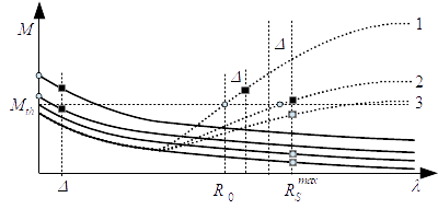
Figure 2 highlights the values of $R^{{\scriptscriptstyle\mathcal{M}}}$ (gray circles) and $R^{{\scriptscriptstyle\mathcal{M}}}_{{\scriptscriptstyle\mathcal{S}}^{\prime}}$ (black squares) related to several possible landscapes of ${\cal M}$. For instance, the landscape corresponding to the top full line, the cell is already in a region with ${\mathcal{M}}>{\mathcal{M}_{th}}$ and so it can hardly move, $R^{{\scriptscriptstyle\mathcal{M}}}=0$ and $R^{{\scriptscriptstyle\mathcal{M}}}_{{\scriptscriptstyle\mathcal{S}}^{\prime}}=\Delta$. The same occurs for the second full line from the top. In this case the cell is very close to the border of the barrier, but still inside it. Conversely, the third full line from the top corresponds to a cell at the border of the physical barrier, but that can look freely ahead. In this case, $R^{{\scriptscriptstyle\mathcal{M}}}=R^{{\scriptscriptstyle\mathcal{M}}}_{{\scriptscriptstyle\mathcal{S}}^{\prime}}=R^{max}_{{\scriptscriptstyle\mathcal{S}}}$. Similarly for the bottom full line. However, looking instead at the top dotted line (line 1), the cell encounters a physical barrier again at $\lambda=R_{0}$, so that $R^{{\scriptscriptstyle\mathcal{M}}}=R_{0}$ and $R^{{\scriptscriptstyle\mathcal{M}}}_{{\scriptscriptstyle\mathcal{S}}^{\prime}}=R_{0}+\Delta$. For the other two dotted lines (numbered as 2 and 3) the cell is barely touching or not encountering yet the barrier, so that $R^{{\scriptscriptstyle\mathcal{M}}}_{{\scriptscriptstyle\mathcal{S}}^{\prime}}=R^{max}_{{\scriptscriptstyle\mathcal{S}}^{\prime}}$.

The dependence of $\mathcal{M}$ on time is due to the fact that the mechanical cue may change in time, for instance because of ECM degradation due to metalloproteinases or redistribution of cell mass in the volume filling case. However, in the following, to simplify a little the notation the dependence on time is usually dropped.

In particular, we remark that

• •

  when the cell center is in a point where $\mathcal{M}<\mathcal{M}_{th}$, it means that it has not reached the physical barrier yet and $R^{{\scriptscriptstyle\mathcal{M}}}>0$;

• •

  when the cell center is in a point where $\mathcal{M}>\mathcal{M}_{th}$, then it means that it is stuck in an overcrowded region and $R^{{\scriptscriptstyle\mathcal{M}}}=0$;

• •

  when the cell center is in a point where $\mathcal{M}=\mathcal{M}_{th}$, unless for very peculiar cases, it means that it is at the border of the barrier. In this case $R^{{\scriptscriptstyle\mathcal{M}}}$ vanishes if the cell is polarized towards the barrier and strictly positive if it wants to move away from it.

We also observe that when the presence of a physical barrier limiting $R_{{\scriptscriptstyle\mathcal{S}}^{\prime}}^{max}$ to $R^{{\scriptscriptstyle\mathcal{M}}}_{{\scriptscriptstyle\mathcal{S}}^{\prime}}(t,{\bf x},\hat{\bf v})$ might also limit $R_{{\scriptscriptstyle\mathcal{S}}}^{max}$ to $R^{{\scriptscriptstyle\mathcal{M}}}_{{\scriptscriptstyle\mathcal{S}}}(t,{\bf x},\hat{\bf v})$.

Summarizing, in order to polarize along the most likely direction $\hat{\bf v}$, the cell with sensing radius $R_{{\scriptscriptstyle\mathcal{S}}}^{max}$ averages the signal $\mathcal{S}$ over a region that is described by a weight function $\gamma_{{\scriptscriptstyle\mathcal{S}}}$ up to $R_{{\scriptscriptstyle\mathcal{S}}}^{max}$, or possibly up to a lower value $R^{{\scriptscriptstyle\mathcal{M}}}_{{\scriptscriptstyle\mathcal{S}}}(t,{\bf x},\hat{\bf v})$ if an obstacle is encountered along its sensing activity. Then, the cell polarized along $\hat{\bf v}$ determines its speed averaging another signal $\mathcal{S}^{\prime}$ through a weight function $\gamma_{{\scriptscriptstyle\mathcal{S}}^{\prime}}$ over the sensing radius $R_{{\scriptscriptstyle\mathcal{S}}^{\prime}}^{max}$ or, as above, up to $R^{{\scriptscriptstyle\mathcal{M}}^{\prime}}_{{\scriptscriptstyle\mathcal{S}}^{\prime}}(t,{\bf x},\hat{\bf v})$.

Coming back to Eq.(11), as in the work by Loy and Preziosi, 2019, it is useful to denote the two factors in it as

$$B[\mathcal{S}]({\bf x},\hat{\bf v})=\int_{0}^{R^{{\scriptscriptstyle\mathcal{M}}}_{{\scriptscriptstyle\mathcal{S}}}({\bf x},\hat{\bf v})}\gamma_{{\scriptscriptstyle\mathcal{S}}}(\lambda)\mathcal{T}_{\lambda}^{\hat{\bf v}}[\mathcal{S}]({\bf x})\,d\lambda\,,$$

(15)

and

$$\Psi[\mathcal{S}^{\prime}]({\bf x},v|\hat{\bf v})=\int_{0}^{R^{{\scriptscriptstyle\mathcal{M}}^{\prime}}_{{\scriptscriptstyle\mathcal{S}}^{\prime}}({\bf x},\hat{\bf v})}\gamma_{{\scriptscriptstyle\mathcal{S}}^{\prime}}(\lambda^{\prime})\psi({\bf x},v|\mathcal{S}^{\prime}({\bf x}+\lambda^{\prime}\hat{\bf v}))\,d\lambda^{\prime}\,,$$

(16)

in order to highlight the directional and the speed sensing and how they affect the choice of the direction and of the speed independently. The turning probability in (10) then reads

$$T[\mathcal{S},\mathcal{S}^{\prime}]({\bf x},v,{\bf v})=c({\bf x})B[\mathcal{S}]({\bf x},\hat{\bf v})\Psi[\mathcal{S}^{\prime}]({\bf x},v|\hat{\bf v}),$$

(17)

where the normalizing constant is

$$c({\bf x})=\dfrac{1}{\displaystyle\int_{\mathbb{S}^{d-1}}B[\mathcal{S}]({\bf x},\hat{\bf v})\Gamma_{{\scriptscriptstyle\mathcal{S}}^{\prime}}({\bf x},\hat{\bf v})\,d\hat{\bf v}\,},$$

(18)

with

$$\Gamma_{{\scriptscriptstyle\mathcal{S}}^{\prime}}({\bf x},\hat{\bf v})=\displaystyle\int_{0}^{R^{{\scriptscriptstyle\mathcal{M}}^{\prime}}_{{\scriptscriptstyle\mathcal{S}}^{\prime}}({\bf x},\hat{\bf v})}\gamma_{{\scriptscriptstyle\mathcal{S}}^{\prime}}(\lambda^{\prime})\,d\lambda^{\prime}.$$

(19)

If $R^{{\scriptscriptstyle\mathcal{M}}^{\prime}}_{{\scriptscriptstyle\mathcal{S}}^{\prime}}$ is independent of $\hat{\bf v}$, then also $\Gamma_{{\scriptscriptstyle\mathcal{S}}^{\prime}}$ is independent of $\hat{\bf v}$ and $c({\bf x})$ can be factorized as $c({\bf x})=c_{1}({\bf x})/\Gamma_{{\scriptscriptstyle\mathcal{S}}^{\prime}}({\bf x})$ with

$$c_{1}({\bf x})=\dfrac{1}{\displaystyle\int_{\mathbb{S}^{d-1}}\int_{0}^{R^{{\scriptscriptstyle\mathcal{M}}}_{{\scriptscriptstyle\mathcal{S}}}({\bf x},\hat{\bf v})}\gamma_{{\scriptscriptstyle\mathcal{S}}}(\lambda)\mathcal{T}_{\lambda}^{\hat{\bf v}}[\mathcal{S}]({\bf x})\,d\lambda\,d\hat{\bf v}},$$

that only depends on the directional sensing.

However, in general, with the definitions (15) and (16), the turning operator (10) writes

$$\mathcal{J}[p]({\bf x},v,{\bf v})=\mu({\bf x})\,\Big(\rho(t,{\bf x})c({\bf x})B[\mathcal{S}]({\bf x},\hat{\bf v})\Psi[\mathcal{S}^{\prime}]({\bf x},v|\hat{\bf v})-p(t,{\bf x},v,{\bf v})\Big)\,,$$

(20)

and the distribution function which nullifies it is

$$p(t,{\bf x},v,{\bf v})=\rho(t,{\bf x})c({\bf x})B[\mathcal{S}]({\bf x},\hat{\bf v})\Psi[\mathcal{S}^{\prime}]({\bf x},v|\hat{\bf v}).$$

(21)

As stated by Loy and Preziosi, 2019, provided that the probability distribution has initially a finite mass and energy and non-absorbing boundary conditions hold, the function (21) is a local stable asymptotic equilibrium state (Bisi et al., 2008; Pettersson, 2004). The related mean velocity is defined by

$${\bf U}_{{\scriptscriptstyle\mathcal{S}},{\scriptscriptstyle\mathcal{S}}^{\prime}}({\bf x})=c({\bf x})\displaystyle\int_{V_{p}}B[\mathcal{S}]({\bf x},\hat{\bf v})\Psi[\mathcal{S}^{\prime}]({\bf x},v|\hat{\bf v}){\bf v}\,dv\,d\hat{\bf v}\,,$$

(22)

and may be rewritten as

$${\bf U}_{{\scriptscriptstyle\mathcal{S}},{\scriptscriptstyle\mathcal{S}}^{\prime}}({\bf x})=c({\bf x})\displaystyle\int_{\mathbb{S}^{d-1}}\Gamma_{{\scriptscriptstyle\mathcal{S}}^{\prime}}({\bf x},\hat{\bf v})B[\mathcal{S}]({\bf x},\hat{\bf v})\,\bar{U}_{{\scriptscriptstyle\mathcal{S}}^{\prime}}({\bf x}|\hat{\bf v})\hat{\bf v}\,d\hat{\bf v}\,,$$

(23)

where

$$\bar{U}_{{\scriptscriptstyle\mathcal{S}}^{\prime}}({\bf x}|\hat{\bf v})=\dfrac{1}{\Gamma_{{\scriptscriptstyle\mathcal{S}}^{\prime}}({\bf x},\hat{\bf v})}\displaystyle\int_{0}^{R^{{\scriptscriptstyle\mathcal{M}}^{\prime}}_{{\scriptscriptstyle\mathcal{S}}^{\prime}}({\bf x},\hat{\bf v})}\gamma_{{\scriptscriptstyle\mathcal{S}}^{\prime}}(\lambda^{\prime})\bar{v}({\bf x}|\mathcal{S}^{\prime}({\bf x}+\lambda^{\prime}\hat{\bf v}))\,d\lambda^{\prime}.$$

(24)

Similarly, the variance-covariance tensor of the transition probability

$$\mathbb{D}_{{\scriptscriptstyle\mathcal{S}},{\scriptscriptstyle\mathcal{S}}^{\prime}}({\bf x})=c({\bf x})\displaystyle\int_{V_{p}}B[\mathcal{S}]({\bf x},\hat{\bf v})\,\Psi[\mathcal{S}^{\prime}]({\bf x},v|\hat{\bf v})({\bf v}-{\bf U}_{{\scriptscriptstyle\mathcal{S}},{\scriptscriptstyle\mathcal{S}}^{\prime}}({\bf x}))\otimes({\bf v}-{\bf U}_{{\scriptscriptstyle\mathcal{S}},{\scriptscriptstyle\mathcal{S}}^{\prime}}({\bf x}))\,\,dv\,d\hat{\bf v}\,,$$

(25)

can be written as

$$\mathbb{D}_{{\scriptscriptstyle\mathcal{S}},{\scriptscriptstyle\mathcal{S}}^{\prime}}({\bf x})=c({\bf x})\displaystyle\int_{\mathbb{S}^{d-1}}\Gamma_{{\scriptscriptstyle\mathcal{S}}^{\prime}}({\bf x},\hat{\bf v})B[\mathcal{S}]({\bf x},\hat{\bf v})\,\bar{D}_{{\scriptscriptstyle\mathcal{S}}^{\prime}}({\bf x}|\hat{\bf v})\hat{\bf v}\otimes\hat{\bf v}\,d\hat{\bf v}-{\bf U}_{{\scriptscriptstyle\mathcal{S}},{\scriptscriptstyle\mathcal{S}}^{\prime}}({\bf x})\otimes{\bf U}_{{\scriptscriptstyle\mathcal{S}},{\scriptscriptstyle\mathcal{S}}^{\prime}}({\bf x})\,,$$

(26)

where

$$\bar{D}_{{\scriptscriptstyle\mathcal{S}}^{\prime}}({\bf x}|\hat{\bf v})=\dfrac{1}{\Gamma_{{\scriptscriptstyle\mathcal{S}}^{\prime}}({\bf x},\hat{\bf v})}\displaystyle\int_{0}^{R^{{\scriptscriptstyle\mathcal{M}}^{\prime}}_{{\scriptscriptstyle\mathcal{S}}^{\prime}}({\bf x},\hat{\bf v})}\gamma_{{\scriptscriptstyle\mathcal{S}}^{\prime}}(\lambda^{\prime})D({\bf x}|\mathcal{S}^{\prime}({\bf x}+\lambda^{\prime}\hat{\bf v}))\,d\lambda^{\prime}.$$

(27)

In order to understand the meaning of $\bar{U}_{{\scriptscriptstyle\mathcal{S}}^{\prime}}$ in the presence of physical limits of migration, let us consider the following case: assume that ahead of a cell there is a space free of obstacles up to a distance $R_{0}$, ${\it e.g.}$, the ECM density has a density yielding a mean speed $\bar{v}_{0}$, while after $R_{0}$ the ECM density is so large to represent a physical limit of migration with a much lower mean speed, say $\bar{\varepsilon}$ or even vanishing with $\bar{v}=0$ and $\psi=\delta(v)$. For sake of simplicity, let us assume that $\gamma_{{\scriptscriptstyle\mathcal{S}}^{\prime}}$ is a Heaviside function. The following interesting cases are possible

• •

  If $R_{0}>R_{{\scriptscriptstyle\mathcal{S}}^{\prime}}^{max}$, then the critical value for $\mathcal{M}$ is located beyond the sensing radius (as for the dashed line 1 in Fig. 2), so that $R^{{\scriptscriptstyle\mathcal{M}}}_{{\scriptscriptstyle\mathcal{S}}^{\prime}}=R^{{\scriptscriptstyle\mathcal{M}}}=R_{{\scriptscriptstyle\mathcal{S}}^{\prime}}^{max}$, and finally $\bar{U}_{{\scriptscriptstyle\mathcal{S}}^{\prime}}=\bar{v}_{0}$;

• •

  If $R_{{\scriptscriptstyle\mathcal{S}}^{\prime}}^{max}-\Delta<R_{0}<R_{{\scriptscriptstyle\mathcal{S}}^{\prime}}^{max}$ (as for the dashed line 2 in Fig. 2), then the critical value for $\mathcal{M}$ is barely sensed with the cell poking a bit in the region with $\mathcal{M}>\mathcal{M}_{th}$. In this case $R^{{\scriptscriptstyle\mathcal{M}}}=R_{0}$ but $R^{{\scriptscriptstyle\mathcal{M}}}_{{\scriptscriptstyle\mathcal{S}}^{\prime}}=R_{{\scriptscriptstyle\mathcal{S}}^{\prime}}^{max}$, so that $\bar{U}_{{\scriptscriptstyle\mathcal{S}}^{\prime}}=\dfrac{\bar{v}_{0}R_{0}+\bar{\varepsilon}(R_{{\scriptscriptstyle\mathcal{S}}^{\prime}}^{max}-R_{0})}{R_{{\scriptscriptstyle\mathcal{S}}^{\prime}}^{max}}$;

• •

  If $R_{0}<R_{{\scriptscriptstyle\mathcal{S}}^{\prime}}^{max}-\Delta$ (as for the dashed line 3 in Fig. 2), then the cell pokes for a depth $\Delta$ into the region with $\mathcal{M}>\mathcal{M}_{th}$. In this case $R^{{\scriptscriptstyle\mathcal{M}}}=R_{0}$ and $R^{{\scriptscriptstyle\mathcal{M}}}_{{\scriptscriptstyle\mathcal{S}}^{\prime}}=R_{0}+\Delta$, so that $\bar{U}_{{\scriptscriptstyle\mathcal{S}}^{\prime}}=\dfrac{\bar{v}_{0}R_{0}+\bar{\varepsilon}\Delta}{R_{0}+\Delta}$;

• •

  In particular, if $R_{0}=0$, the cell has arrived at the barrier, then $R^{{\scriptscriptstyle\mathcal{M}}}=0$ and $R^{{\scriptscriptstyle\mathcal{M}}}_{{\scriptscriptstyle\mathcal{S}}^{\prime}}=\Delta$, so that $\bar{U}_{{\scriptscriptstyle\mathcal{S}}^{\prime}}=\bar{\varepsilon}$. Hence, in the limit $\Delta\to 0$ when the cell is approaching the physical limit, its speed decreases fast to $\bar{\varepsilon}$, which can also be taken to be zero, as in the simulations to follow;

• •

  Conversely, if the cell is so close to an exit, say at a distance $R_{exit}\in[0,\Delta]$, that it can sense outside the physical barrier, then $R_{0}=0$ and $R^{{\scriptscriptstyle\mathcal{M}}}_{{\scriptscriptstyle\mathcal{S}}^{\prime}}=\Delta$, so that $\bar{U}_{{\scriptscriptstyle\mathcal{S}}^{\prime}}=\bar{v}_{0}-(\bar{v}_{0}-\bar{\varepsilon})\dfrac{R_{exit}}{\Delta}$ Hence, in the limit $\Delta\to 0$ its speed increases fast to $\bar{v}_{0}$.

Figure 3 gives an example of the measured $\bar{U}_{{\scriptscriptstyle\mathcal{S}}^{\prime}}$ as a function of the cell position (with the cell polarized to move to the right) when the region with $\mathcal{M}>\mathcal{M}_{th}$ is the interval $(a,b)$. The cell moves at a velocity $\bar{v}_{0}$ till it reaches a distance $R^{max}_{{\scriptscriptstyle\mathcal{S}}^{\prime}}$ from the barrier. Then it decreases its speed at first only sligthly and then faster when getting closer to the barrier to reach a very small or vanishing value. If on the other hand the cell is at the right border of the barrier it can move freely with velocity $\bar{v}_{0}$.

In the simulations to follow, in order to test the physical limit of migration, we shall always consider $\Delta=\bar{\varepsilon}=0$, ${\it i.e.}$, the case in which the cell can not poke in the limited area. We leave to a future work the investigation of the effect of considering a non-vanishing $\Delta$.

One of the main issues about transport equations consists in recovering the appropriate macroscopic limit allowing to highlight the driving macroscopic phenomenon. Typically these are obtained by identifying a small parameter $\epsilon\ll 1$ that allows to suitably rescale the transport equation with a parabolic or a hyperbolic scaling. These correspond, respectively, to

$$\begin{array}[]{lr}\tau=\epsilon^{2}t,\quad{\bf\boldsymbol{\xi}}=\epsilon{\bf x},\\[8.0pt] \tau=\epsilon t,\quad{\bf\boldsymbol{\xi}}=\epsilon{\bf x}.\end{array}$$

The proper choice of the time scale comes from a nondimensionalization of the turning operator (10). Referring to the functions introduced in (15) and (16), we suppose that, up to a nondimensionalization, $B[\mathcal{S}]$ and $\Psi[\mathcal{S}^{\prime}]$ may be written as

$$B[\mathcal{S}]=B[\mathcal{S}]_{0}+\epsilon B[\mathcal{S}]_{1}+\mathcal{O}(\epsilon^{2}),$$

$$\Psi[\mathcal{S}^{\prime}]=\Psi[\mathcal{S}^{\prime}]_{0}+\epsilon\Psi[\mathcal{S}^{\prime}]_{1}+\mathcal{O}(\epsilon^{2}),$$

which describe different orders of bias. Then, the turning kernel $T[\mathcal{S},\mathcal{S}^{\prime}]$ can be written as

$$T[\mathcal{S},\mathcal{S}^{\prime}](\boldsymbol{\xi},v,\hat{{\bf v}})=T[\mathcal{S},\mathcal{S}^{\prime}]_{0}(\boldsymbol{\xi},v,\hat{{\bf v}})+\epsilon T[\mathcal{S},\mathcal{S}^{\prime}]_{1}(\boldsymbol{\xi},v,\hat{{\bf v}})+\mathcal{O}(\epsilon^{2}),$$

(28)

where

$$T[\mathcal{S},\mathcal{S}^{\prime}]_{0}(v,\hat{{\bf v}})=c({\bf x})B[\mathcal{S}]_{0}(\hat{\bf v})\Psi[\mathcal{S}^{\prime}]_{0}(v|\hat{\bf v}),$$

(29)

and

$$T[\mathcal{S},\mathcal{S}^{\prime}]_{1}(v,\hat{{\bf v}})=c({\bf x})B[\mathcal{S}]_{0}(\hat{\bf v})\Psi[\mathcal{S}^{\prime}]_{1}(v|\hat{\bf v})+c({\bf x})B[\mathcal{S}]_{1}(\hat{\bf v})\Psi[\mathcal{S}^{\prime}]_{0}(v|\hat{\bf v})\,.$$

(30)

Coherently, the means and variances of $\Psi[\mathcal{S}^{\prime}]_{0}$ and $\Psi[\mathcal{S}^{\prime}]_{1}$ will be, respectively, denoted by $\bar{U}_{{\scriptscriptstyle\mathcal{S}}^{\prime}}^{0}$, $\bar{U}_{{\scriptscriptstyle\mathcal{S}}^{\prime}}^{1}$, $\bar{D}_{{\scriptscriptstyle\mathcal{S}}^{\prime}}^{0}$, $\bar{D}_{{\scriptscriptstyle\mathcal{S}}^{\prime}}^{1}$. Similarly, the distribution function $p$ is expanded as

$$p=p_{0}+\epsilon p_{1}+\mathcal{O}(\epsilon^{2}).$$

(31)

As there is conservation of mass we have that (Othmer and Hillen, 2000) all the mass is in $p_{0}$, ${\it i.e.}$,

$$\rho_{0}=\rho,\quad\rho_{i}=0\quad\forall i\geq 1\,,$$

(32)

where $\displaystyle{\rho_{i}=\int_{V_{p}}p_{i}\,dv\,d\hat{{\bf v}}}$. Furthermore, for performing the diffusive limit we shall suppose that $\displaystyle{\int_{V_{p}}p_{i}v\hat{{\bf v}}\,dv\,d\hat{{\bf v}}=0}\quad\forall i\geq 2$.

If we suppose that

$$\displaystyle\int_{0}^{U}\Psi[\mathcal{S}^{\prime}]_{0}(v|\hat{\bf v})\,dv=\displaystyle\int_{0}^{U}\Psi[\mathcal{S}^{\prime}](v|\hat{\bf v})\,dv\,,\qquad\displaystyle\int_{0}^{U}\Psi[\mathcal{S}^{\prime}]_{i}(v|\hat{\bf v})\,dv=0\quad\forall i\geq 1,$$

and

$$\displaystyle\int_{\mathbb{S}^{d-1}}B[\mathcal{S}]_{0}(\hat{\bf v})\,d\hat{\bf v}=\int_{\mathbb{S}^{d-1}}B[\mathcal{S}](\hat{\bf v})\,d\hat{\bf v}\,,\qquad\int_{\mathbb{S}^{d-1}}B[\mathcal{S}]_{i}(\hat{\bf v})\,d\hat{\bf v}=0\quad\forall i\geq 1,$$

then

	$$\displaystyle\int_{V_{p}}T[\mathcal{S},\mathcal{S}^{\prime}]_{0}(\boldsymbol{\xi},v,\hat{{\bf v}})\,dv\,d\hat{{\bf v}}=1,$$		(33a)
and
	$$\displaystyle\int_{V_{p}}T[\mathcal{S},\mathcal{S}^{\prime}]_{i}(\boldsymbol{\xi},v,\hat{{\bf v}})\,dv\,d\hat{{\bf v}}=0\quad\forall i\geq 1,$$		(33b)

that are needed for performing a macroscopic limit (Othmer and Hillen, 2000).

Denoting by $\mathcal{J}^{i}$ the turning operators defined by $T[\mathcal{S},\mathcal{S}^{\prime}]_{i}$, it turns out for instance that

$$\mathcal{J}^{0}[p_{0}](v,\hat{{\bf v}})=\mu(\rho_{0}T[\mathcal{S},\mathcal{S}^{\prime}]_{0}(v,\hat{{\bf v}})-p_{0}(v,\hat{{\bf v}}))=0\,,$$

(34)

and therefore the function $p_{0}$ is the equilibrium function given by

$$p_{0}({\bf v}_{p})=\rho_{0}T[\mathcal{S},\mathcal{S}^{\prime}]_{0}(v,\hat{{\bf v}}).$$

(35)

The velocity and tensor of the second moments of the transition probability then naturally write as

$${\bf U}_{\scriptscriptstyle\mathcal{S},\mathcal{S^{\prime}}}={\bf U}_{\scriptscriptstyle\mathcal{S},\mathcal{S^{\prime}}}^{0}+\epsilon{\bf U}_{\scriptscriptstyle\mathcal{S},\mathcal{S^{\prime}}}^{1}+\mathcal{O}(\epsilon^{2})\,,$$

(36)

and

$$\mathbb{D}_{\scriptscriptstyle\mathcal{S},\mathcal{S^{\prime}}}=\mathbb{D}_{\scriptscriptstyle\mathcal{S},\mathcal{S^{\prime}}}^{0}+\epsilon\mathbb{D}_{\scriptscriptstyle\mathcal{S},\mathcal{S^{\prime}}}^{1}+\mathcal{O}(\epsilon^{2})\,,$$

(37)

where

$${\bf U}_{\scriptscriptstyle\mathcal{S},\mathcal{S^{\prime}}}^{i}=\displaystyle\int_{V_{p}}T[\mathcal{S},\mathcal{S}^{\prime}]_{i}{\bf v}\,dv\,d\hat{{\bf v}}\,,$$

and

$$\mathbb{D}_{\scriptscriptstyle\mathcal{S},\mathcal{S^{\prime}}}^{i}=\displaystyle\int_{V_{p}}T[\mathcal{S},\mathcal{S}^{\prime}]_{i}({\bf v}-{\bf U}_{\scriptscriptstyle\mathcal{S},\mathcal{S^{\prime}}}^{i})\otimes({\bf v}-{\bf U}_{\scriptscriptstyle\mathcal{S},\mathcal{S^{\prime}}}^{i})\,dv\,d\hat{{\bf v}}\,,$$

for $i\geq 0$. Then, using (29) and (30), the macroscopic velocity of order 0 is

$${\bf U}_{{\scriptscriptstyle\mathcal{S}},{\scriptscriptstyle\mathcal{S}}^{\prime}}^{0}(\boldsymbol{\xi})=c(\boldsymbol{\xi})\int_{\mathbb{S}^{d-1}}\Gamma_{{\scriptscriptstyle\mathcal{S}}^{\prime}}(\boldsymbol{\xi},\hat{\bf v})B[\mathcal{S}]_{0}(\hat{\bf v})\,\bar{U}_{{\scriptscriptstyle\mathcal{S}}^{\prime}}^{0}(\boldsymbol{\xi}|\hat{\bf v})\hat{\bf v}\,d\hat{\bf v}\,,$$

(38)

that of order 1 is

$${\bf U}_{{\scriptscriptstyle\mathcal{S}},{\scriptscriptstyle\mathcal{S}}^{\prime}}^{1}(\boldsymbol{\xi})=c(\boldsymbol{\xi})\int_{\mathbb{S}^{d-1}}\Gamma_{{\scriptscriptstyle\mathcal{S}}^{\prime}}(\boldsymbol{\xi},\hat{\bf v})\Big(B[\mathcal{S}]_{0}(\hat{\bf v})\bar{U}_{{\scriptscriptstyle\mathcal{S}}^{\prime}}^{1}(\boldsymbol{\xi}|\hat{\bf v})+B[\mathcal{S}]_{1}(\hat{\bf v})\bar{U}_{{\scriptscriptstyle\mathcal{S}}^{\prime}}^{0}(\boldsymbol{\xi}|\hat{\bf v})\Big)\hat{\bf v}\,d\hat{\bf v}$$

(39)

and the equilibrium diffusion tensor is

$$\mathbb{D}_{{\scriptscriptstyle\mathcal{S}},{\scriptscriptstyle\mathcal{S}}^{\prime}}({\bf x})=c(\boldsymbol{\xi})\displaystyle\int_{\mathbb{S}^{d-1}}\Gamma_{{\scriptscriptstyle\mathcal{S}}^{\prime}}(\boldsymbol{\xi},\hat{\bf v})B[\mathcal{S}]_{0}(\boldsymbol{\xi},\hat{\bf v})\,\bar{D}_{{\scriptscriptstyle\mathcal{S}}^{\prime}}^{0}(\boldsymbol{\xi}|\hat{\bf v})\hat{\bf v}\otimes\hat{\bf v}\,d\hat{\bf v}-{\bf U}_{{\scriptscriptstyle\mathcal{S}},{\scriptscriptstyle\mathcal{S}}^{\prime}}^{0}(\boldsymbol{\xi})\otimes{\bf U}_{{\scriptscriptstyle\mathcal{S}},{\scriptscriptstyle\mathcal{S}}^{\prime}}^{0}(\boldsymbol{\xi})\,,$$

(40)

where

$$\bar{D}_{{\scriptscriptstyle\mathcal{S}}^{\prime}}^{0}(\boldsymbol{\xi}|\hat{\bf v})=\dfrac{1}{\Gamma_{{\scriptscriptstyle\mathcal{S}}^{\prime}}(\boldsymbol{\xi},\hat{\bf v})}\displaystyle\int_{0}^{R^{\mathcal{M}^{\prime}}_{{\scriptscriptstyle\mathcal{S}}^{\prime}}(\boldsymbol{\xi},\hat{\bf v})}\gamma_{{\scriptscriptstyle\mathcal{S}}^{\prime}}(\lambda^{\prime})D^{0}(\boldsymbol{\xi}|\mathcal{S}^{\prime}(\boldsymbol{\xi}+\lambda^{\prime}\hat{\bf v}))\,d\lambda^{\prime}.$$

The diffusion tensor is in general anisotropic, as $\bar{D}_{{\scriptscriptstyle\mathcal{S}}^{\prime}}^{0}$ may be non isotropic in $\hat{\bf v}$.

The discriminating factor on which scaling can be performed is whether $T$ is such that

$${\bf U}_{{\scriptscriptstyle\mathcal{S}},{\scriptscriptstyle\mathcal{S}}^{\prime}}^{0}=\textbf{0}$$

(41)

${\it i.e.}$, the leading order macroscopic velocity vanishes, or not. This is the necessary functional condition for performing a diffusive limit, and it is actually what we expect in a diffusive regime. Referring to Eq. (38), we observe that, even in the case in which $B[\mathcal{S}]$ is constant, corresponding for instance to no directional bias and $R_{{\scriptscriptstyle\mathcal{S}}^{\prime}}^{{\scriptscriptstyle\mathcal{M}}^{\prime}}$, and therefore $\Gamma_{{\scriptscriptstyle\mathcal{S}}^{\prime}}$ not depending on $\hat{{\bf v}}$, Eq. (41) is satisfied if the mean velocity $\bar{U}_{{\scriptscriptstyle\mathcal{S}}^{\prime}}^{0}(\boldsymbol{\xi}|\hat{\bf v})$ is even as a function of $\hat{{\bf v}}$ for $a.e.\ \boldsymbol{\xi}\in\Omega$. Moreover, if $R_{{\scriptscriptstyle\mathcal{S}}^{\prime}}^{{\scriptscriptstyle\mathcal{M}}^{\prime}}$ depends on $\hat{{\bf v}}$, condition (41) can not be satisfied, unless for trivial cases that do not include physical limits of migration, as we will illustrate in the next sections through some examples. Therefore, in general one can only perform a hyperbolic limit which reads

$$\dfrac{\partial\rho}{\partial\tau}+\nabla\cdot\big(\rho{\bf U}_{{\scriptscriptstyle\mathcal{S}},{\scriptscriptstyle\mathcal{S}}^{\prime}}^{0}\big)=0\,.$$

(42)

In order to see which regimes are diffusive or hyperbolic, it is instructive to see what happens if $R_{{\scriptscriptstyle\mathcal{S}}^{\prime}}({\bf x},\hat{\bf v})$ is much smaller then the characteristic length of variation of $\mathcal{S}^{\prime}$ as done by Loy and Preziosi, 2019 for the directional bias. In this case, we can expand $\mathcal{S}^{\prime}$ as

$$\mathcal{S}^{\prime}({\bf x}+\lambda^{\prime}\hat{{\bf v}})=\mathcal{S}^{\prime}({\bf x})+\lambda^{\prime}\hat{\bf v}\cdot\nabla\mathcal{S}^{\prime}({\bf x})+\mathcal{O}(\lambda^{\prime 2})\quad\forall\lambda^{\prime}\leq R_{{\scriptscriptstyle\mathcal{S}}^{\prime}}({\bf x},\hat{\bf v})$$

(43)

and we have that that the quantity $\mathcal{S}^{\prime}({\bf x})+\lambda^{\prime}\hat{\bf v}\cdot\nabla\mathcal{S}^{\prime}({\bf x})$ stays positive. The density function $\psi(v|\mathcal{S}^{\prime}({\bf y}))$, ${\bf y}\in\Omega$ may be seen as a function of two variables

$$\tilde{\psi}:(v,{\bf y})\in[0,U]\times\Omega\longmapsto\tilde{\psi}(v,{\bf y})=\psi(v|\mathcal{S}^{\prime}({\bf y}))$$

composed with the function $\mathcal{S}^{\prime}$ defined on $\Omega$. If we suppose that $\tilde{\psi}\in L^{1}([0,U])\times C^{2}(\Omega)$ with

$$\int_{0}^{U}\tilde{\psi}(v,{\bf y})dv=\int_{0}^{U}\psi(v|\mathcal{S}^{\prime}({\bf y}))dv=1,$$

(44)

then, in virtue of (43) we may write

	$\displaystyle\tilde{\psi}(v,\mathcal{S}^{\prime}({\bf x}+\lambda^{\prime}\hat{\bf v}))$	$\displaystyle=$	$\displaystyle\tilde{\psi}(v,\mathcal{S}^{\prime}({\bf x})+\lambda^{\prime}\hat{\bf v}\cdot\nabla\mathcal{S}^{\prime}({\bf x})+\mathcal{O}(\lambda^{\prime 2}))$
		$\displaystyle=$	$\displaystyle\tilde{\psi}(v,\mathcal{S}^{\prime}({\bf x}))+\dfrac{\partial}{\partial\mathcal{S}^{\prime}}[\tilde{\psi}(v,\mathcal{S}^{\prime}({\bf x}))]\lambda^{\prime}\hat{\bf v}\cdot\nabla\mathcal{S}^{\prime}({\bf x})+\mathcal{O}(\lambda^{\prime 2})\quad\forall\lambda^{\prime}\leq R_{{\scriptscriptstyle\mathcal{S}}^{\prime}}({\bf x},\hat{\bf v}).$

Therefore, recalling Eqs.(17) and (18) the transition probability writes

	$\displaystyle T({\bf x},v,\hat{\bf v})$	$\displaystyle=$	$\displaystyle\dfrac{B[\mathcal{S}](\hat{\bf v})}{\displaystyle{\int_{\mathbb{S}^{d-1}}B[\mathcal{S}](\hat{\bf v})\Gamma_{{\scriptscriptstyle\mathcal{S}}^{\prime}}({\bf x},\hat{{\bf v}})\,d\hat{\bf v}}}\int_{0}^{R_{{\scriptscriptstyle\mathcal{S}}^{\prime}}({\bf x},\hat{\bf v})}\gamma_{{\scriptscriptstyle\mathcal{S}}^{\prime}}(\lambda^{\prime})\psi(v|\mathcal{S}^{\prime}({\bf x}+\lambda^{\prime}\hat{\bf v}))\,d\lambda^{\prime}$
		$\displaystyle\approx$	$\displaystyle\dfrac{B[\mathcal{S}](\hat{\bf v})\Gamma_{{\scriptscriptstyle\mathcal{S}}^{\prime}}({\bf x},\hat{{\bf v}})}{\displaystyle{\int_{\mathbb{S}^{d-1}}B[\mathcal{S}](\hat{\bf v})\Gamma_{{\scriptscriptstyle\mathcal{S}}^{\prime}}({\bf x},\hat{{\bf v}})\,d\hat{\bf v}}}\left[\psi(v|\mathcal{S}^{\prime}({\bf x}))+\Lambda^{\prime}({\bf x},\hat{\bf v})\dfrac{\partial}{\partial\mathcal{S}^{\prime}}[\psi(v|\mathcal{S}^{\prime}({\bf x}))]\nabla\mathcal{S}^{\prime}({\bf x})\cdot\hat{\bf v}\right]$

where

$$\Lambda^{\prime}({\bf x},\hat{{\bf v}})=\dfrac{1}{\Gamma_{{\scriptscriptstyle\mathcal{S}}^{\prime}}({\bf x},\hat{{\bf v}})}\int_{0}^{R_{{\scriptscriptstyle\mathcal{S}}^{\prime}}({\bf x},\hat{\bf v})}\gamma_{{\scriptscriptstyle\mathcal{S}}^{\prime}}(\lambda^{\prime})\lambda^{\prime}\,d\lambda^{\prime}.$$

The quantity

$$\dfrac{\partial}{\partial\mathcal{S}^{\prime}}\bar{v}({\bf x}|\mathcal{S}^{\prime}({\bf x}))$$

is the derivative of the master curve relating $\bar{v}$ to the signal $\mathcal{S}^{\prime}$.

References

- Abercrombie and Heaysman, (1953) Abercrombie, M. and Heaysman, J. E. (1953). Observations on the social behaviour of cells in tissue culture: I. Speed of movement of chick heart fibroblasts in relation to their mutual contacts. Experimental Cell Research, 5(1):111 – 131.
- Adler, (1966) Adler, J. (1966). Chemotaxis in bacteria. Science, 153(3737):708–116.
- Alt, (1980) Alt, W. (1980). Biased random walk models for chemotaxis and related diffusion approximations. Journal of Mathematical Biology, 9(2):147–177.
- Arduino and Preziosi, (2015) Arduino, A. and Preziosi, L. (2015). A multiphase model of tumour segregation in situ by a heterogeneous extracellular matrix. International Journal of Non-Linear Mechanics, 75:22–30.
- Armstrong et al., (2006) Armstrong, N. J., Painter, K. J., and Sherratt, J. A. (2006). A continuum approach to modelling cell-cell adhesion. Journal of Theoretical Biology, 243(1):98–113.
- Bisi et al., (2008) Bisi, M., Carrillo, J. A., and Lods, B. (2008). Equilibrium solution to the inelastic Boltzmann equation driven by a particle bath. Journal of Statistical Physics, 133(5):841–870.
- Bitsouni and Eftimie, (2018) Bitsouni, V. and Eftimie, R. (2018). Non-local parabolic and hyperbolic models for cell polarisation in heterogeneous cancer cell populations. Bulletin of Mathematical Biology, 80(10):2600–2632.
- Block et al., (1983) Block, S. M., Segall, J. E., and Berg, H. C. (1983). Adaptation kinetics in bacterial chemotaxis. Journal of Bacteriology, 154(1):312–323.
- Buttenschön et al., (2018) Buttenschön, A., Hillen, T., Gerisch, A., and Painter, K. J. (2018). A space-jump derivation for non-local models of cell-cell adhesion and non-local chemotaxis. Journal of Mathematical Biology, 76(1):429–456.
- Carrillo et al., (2015) Carrillo, J., Hoffmann, F., and Eftimie, R. (2015). Non-local kinetic and macroscopic models for self-organised animal aggregations. Kinetic Related Models, 8:413–441.
- Cercignani, (1987) Cercignani, C. (1987). The Boltzmann Equation and its Applications. Springer, New York.
- (12) Chauviere, A., Hillen, T., and Preziosi, L. (2007a). Modeling cell movement in anisotropic and heterogeneous network tissues. Networks Heterogeneous Media, 2(2):333–357.
- (13) Chauviere, A., Hillen, T., and Preziosi, L. (2007b). Modeling the motion of a cell population in the extracellular matrix. Discrete and Continuous Dynamical Systems B, 2007(Supplemental volume):250–259.
- Colombi et al., (2017) Colombi, A., Scianna, M., and Preziosi, L. (2017). Coherent modelling switch between pointwise and distributed representations of cell aggregates. Journal of Mathematical Biology, 74(4):783–808.
- Colombi et al., (2015) Colombi, A., Scianna, M., and Tosin, A. (2015). Differentiated cell behavior: a multiscale approach using measure theory. Journal of Mathematical Biology, 71:1049–1079.
- Davidson et al., (2014) Davidson, P. M., Denais, C., Bakshi, M. C., and Lammerding, J. (2014). Nuclear deformability constitutes a rate-limiting step during cell migration in 3-d environments. Cellular and Molecular Bioengineering, 7(3):293–306.
- Devreotes and Janetopoulos, (2003) Devreotes, P. and Janetopoulos, C. (2003). Eukaryotic chemotaxis: Distinctions between directional sensing and polarization. Journal of Biological Chemistry, 278(23):20445–20448.
- Eftimie, (2012) Eftimie, R. (2012). Hyperbolic and kinetic models for self-organized biological aggregations and movement: a brief review. Journal of Mathematical Biology, 65(1):35–75.
- Eftimie et al., (2017) Eftimie, R., Perez, M., and Buono, P.-L. (2017). Pattern formation in a nonlocal mathematical model for the multiple roles of the tgf- pathway in tumour dynamics. Mathematical Biosciences, 289:96 – 115.
- Friedl et al., (2011) Friedl, P., Wolf, K., and Lammerding, J. (2011). Nuclear mechanics during cell migration. Current Opinion in Cell Biology, 1:55–64.
- Giverso et al., (2017) Giverso, C., Arduino, A., and Preziosi, L. (2017). How nucleus mechanics and ECM microstructure influence the invasion of single cells and multicellular aggregates. Bulletin of Mathematical Biology, 80:1–29.
- Giverso et al., (2014) Giverso, C., Grillo, A., and Preziosi, L. (2014). Influence of nucleus deformability on cell entry into cylindrical structures. Biomechanics and Modeling in Mechanobiology, 13:481–502.
- Goodman et al., (1989) Goodman, S. L., Risse, G., and Mark, K. (1989). The E8 subfragment of laminin promotes locomotion of myoblasts over extracellular matrix. The Journal of Cell Biology, 109:799–809.
- Harley et al., (2008) Harley, B., Kim, H., Zaman, M., Yannas, I., Lauffenburger, D., and Gibson, L. J. (2008). Microarchitecture of three-dimensional scaffolds influences cell migration behavior via junction interactions. Biophysical journal, 95(8):4013–4024.
- Hillen, (2006) Hillen, T. (2006). M5 mesoscopic and macroscopic models for mesenchymal motion. Journal of Mathematical Biology, 53:585–616.
- Hillen et al., (2007) Hillen, T., Painter, K. J., and Schmeiser, C. (2007). Global existence for chemotaxis with finite sampling radius. Discrete Continuous Dynamical Systems - B, 7(1):125–144.
- Lods, (2005) Lods, B. (2005). Semigroup generation propertiesof streaming operators with noncontractive boundary conditions. Mathematical and Computer Modelling, 42:1441–1462.
- Loy and Preziosi, (2019) Loy, N. and Preziosi, L. (2019). Kinetic models with non-local sensing determining cell polarization and speed according to independent cues. Journal of Mathematical Biology-accepted (arXiv:1906.11039v3).
- Nam et al., (2016) Nam, K.-H., Kim, P., K. Wood, D., Kwon, S., P. Provenzano, P., and Kim, D.-H. (2016). Multiscale cues drive collective cell migration. Scientific Reports, 6:29749.
- Othmer and Hillen, (2002) Othmer, H. and Hillen, T. (2002). The diffusion limit of transport equations ii: Chemotaxis equations. SIAM Journal of Applied Mathematics, 62:1222–1250.
- Othmer and Stevens, (2001) Othmer, H. and Stevens, A. (2001). Aggregation, blowup, and collapse: The ABC’s of taxis in reinforced random walks. SIAM Journal on Applied Mathematics, 57:311–338.
- Othmer et al., (1988) Othmer, H. G., Dunbar, S. R., and Alt, W. (1988). Models of dispersal in biological systems. Journal of Mathematical Biology, 26(3):263–298.
- Othmer and Hillen, (2000) Othmer, H. G. and Hillen, T. (2000). The diffusion limit of transport equations derived from velocity-jump processes. SIAM Journal of Applied Mathematics, 61:751–775.
- Painter and Hillen, (2002) Painter, J. K. and Hillen, T. (2002). Volume-filling and quorum-sensing in models for chemosensitive movement. Canadian Applied Mathematics Quarterly, 10:501–543.
- Painter et al., (2010) Painter, K. J., Armstrong, N. J., and Sherratt, J. A. (2010). The impact of adhesion on cellular invasion processes in cancer and development. Journal of Theoretical Biology, 264(3):1057–1067.
- Painter et al., (2015) Painter, K. J., Bloomfield, M. J., Sherratt, J. A., and Gerisch, A. (2015). A nonlocal model for contact attraction and repulsion in heterogeneous cell populations. Bulletin of Mathematical Biology, 77:1132–1165.
- Painter and Sherratt, (2003) Painter, K. J. and Sherratt, J. A. (2003). Modelling the movement of interacting cell populations. Journal of Theoretical Biology, 225(3):327–339.
- Palcewski, (1992) Palcewski, A. (1992). Velocity averaging for boundary value problems. Series on Advances in Mathematics For Applied Sciences. World Scientific Publishing Company.
- Pettersson, (2004) Pettersson, R. (2004). On solutions to the linear Boltzmann equation for granular gases. Transport Theory and Statistical Physics, 33(5-7):527–543.
- Peyton and Putnam, (2005) Peyton, S. R. and Putnam, A. J. (2005). Extracellular matrix rigidity governs smooth muscle cell motility in a biphasic fashion. Journal of Cellular Physiology, 204(1):198–209.
- Plaza, (2019) Plaza, R. G. (2019). Derivation of a bacterial nutrient-taxis system with doubly degenerate cross-diffusion as the parabolic limit of a velocity-jump process. Journal of Mathematical Biology, 78:1681–1711.
- Schmeiser and Nouri, (2017) Schmeiser, C. and Nouri, A. (2017). Aggregated steady states of a kinetic model for chemotaxis. Kinetic and Related Models, 10(1):313 – 327.
- Schoumacher et al., (2010) Schoumacher, M., Goldman, R. D., Louvard, D., and Vignjevic, D. M. (2010). Actin, microtubules, and vimentin intermediate filaments cooperate for elongation of invadopodia. The Journal of Cell Biology, 189(3):541–556.
- Scianna and Preziosi, (2013) Scianna, M. and Preziosi, L. (2013). Modeling the influence of nucleus elasticity on cell invasion in fiber networks and microchannels. Journal of Theoretical Biology, 317:394 – 406.
- Scianna and Preziosi, (2014) Scianna, M. and Preziosi, L. (2014). A cellular Potts model for the MMP-dependent and-independent cancer cell migration in matrix microtracks of different dimensions. Computational Mechanics, 53:485–497.
- Scianna et al., (2013) Scianna, M., Preziosi, L., and Wolf, K. (2013). A cellular Potts model simulating cell migration on and in matrix environments. Mathematical Biosciences and Engineering, 10:235–261.
- Shankar et al., (2010) Shankar, J., Messenberg, A., Chan, J., Underhill, T. M., Foster, L. J., and Nabi, I. R. (2010). Pseudopodial actin dynamics control epithelial-mesenchymal transition in metastatic cancer cells. Cancer Research, 70(9):3780–3790.
- Stroock, (1974) Stroock, D. W. (1974). Some stochastic processes which arise from a model of the motion of a bacterium. Zeitschrift für Wahrscheinlichkeitstheorie und Verwandte Gebiete, 28(4):305–315.
- te Boekhorst et al., (2016) te Boekhorst, V., Preziosi, L., and Friedl, P. (2016). Plasticity of cell migration in vivo and in silico. Annual Review of Cell and Developmental Biology, 32:491–526.
- Tosin and Frasca, (2011) Tosin, A. and Frasca, P. (2011). Existence and approximation of probability measure solutions to models of collective behaviors. Networks Heterogeneous Media, 6(1):561–596.
- Wolf et al., (2013) Wolf, K., Te Lindert, M., Vortmeyer-Krause, M., Alexander, S., te Riet, J., L Willis, A., M Hoffman, R., Figdor, C., J Weiss, S., and Friedl, P. (2013). Physical limits of cell migration: Control by ECM space and nuclear deformation and tuning by proteolysis and traction force. The Journal of Cell Biology, 201:1069–1084.
- Wolf et al., (2007) Wolf, K., Wu, Y. I., Liu, Y., Geiger, J., Tam, E., Overall, C., Stack, M. S., and Friedl, P. (2007). Multi-step pericellular proteolysis controls the transition from individual to collective cancer cell invasion. Nature Cell Biology, 9(8):893–904.
- Zaman et al., (2006) Zaman, M. H., Trapani, L. M., Sieminski, A. L., Mackellar, D., Gong, H., Kamm, R. D., Wells, A., Lauffenburger, D. A., and Matsudaira, P. (2006). Migration of tumor cells in 3D matrices is governed by matrix stiffness along with cell-matrix adhesion and proteolysis. Proceedings of the National Academy of Sciences of the United States of America, 103(29):10889–10894.