Electron-positron pair production in frequency modulated laser fields

Generally, there are two different mechanisms that can induce electron-positron pair creation from vacuum. One is the Schwinger effect (tunneling mechanism) and the other one is the multiphoton absorption. These two mechanisms can be well distinguished by the adiabaticity parameter $\gamma=m\omega/|e|E_{0}$ Brezin1970. For the former one $\gamma\ll 1$ and for the latter one $\gamma\gg 1$. While in this paper we are focused on the interesting intermediate regime $\gamma\sim\mathcal{O}(1)$. For instance, the adiabaticity parameter $\gamma=5$ for the modulated field with $E_{0}=0.1E_{\mathrm{cr}}$ and $\omega=0.5m$.

Figure 2 shows the momentum spectrum of created particles in frequency modulated fields with different modulation parameters. It can be seen that the momentum spectra in the modulated field have obvious interference pattern. To understand this interference effect, we show the peak positions of the momentum spectra labeled as $1$, $2$, …, and $19$ on Fig. 2 in Tab. 1. According to the definition of total energy of a created electron, the total energy of created electron-positron pairs is

where $m_{\ast}=m\sqrt{1+\frac{e^{2}}{m^{2}}\frac{E_{0}^{2}}{2\omega^{2}}}$ is called effective mass Christian2014. So the total energy $E_{1}$, $E_{2}$, …, and $E_{19}$ which correspond to the momentum peak $p_{1}$, $p_{2}$, …, and $p_{19}$ can be calculated by the above equation. For example, in Fig. 2 (a), we can obtain the total energy $E_{1}=2.02$ and $E_{2}=2.49$ according to Eq. (5). Furthermore, we find that $E_{1}\approx 4\omega_{0}$ and $E_{2}\approx 5\omega_{0}$, so according to the energy conservation the created particles with momentum $p_{1}$ and $p_{2}$ correspond to four- and five-photon absorption process, respectively. And the number of created particles by four-photon absorption is much greater than that by five-photon absorption.

For Figs. 2 (b) and (c), the modulation frequency $\omega_{m}$ is $0.07m$ and $0.1m$, respectively. Due to the fact that $E_{3},E_{9}\approx 2.02\approx 4\omega_{0}$ and $E_{8},E_{14}\approx 2.50=5\omega_{0}$, the created pairs with momentum $p_{3}$ and $p_{9}$ correspond to four-photon absorption and the created particles with momentum $p_{8}$ and $p_{14}$ correspond to five-photon absorption process. In addition to these momentum peaks corresponding to four- and five-photon absorption, one can also see that there are other momentum peaks in Figs. 2 (b) and (c). For Fig. 2 (b) where the modulation frequency $\omega_{m}=0.07m$, the total energy of created pairs $E_{4}\sim E_{7}$ corresponding to momentum peaks $p_{4}\sim p_{7}$ are $2.07$, $2.14$, $2.21$ and $2.28$, respectively. Based on energy conservation, these momentum peaks are still caused by four-photon absorption process, because $E_{4}\approx 3\omega_{0}+\omega_{1}$, $E_{5}\approx 3\omega_{0}+\omega_{2}$, $E_{6}\approx 3\omega_{0}+\omega_{3}$ and $E_{7}\approx 3\omega_{0}+\omega_{4}$. By the way, since the original frequency dominates the frequency components of the modulated electric field, a large number of photons with frequency $\omega_{0}$ is absorbed in pair creation. Similar to the above discussions, for Fig. 2 (c) with the modulation frequency $\omega_{m}=0.1m$, the total energy of created pairs $E_{10}\sim E_{13}$ corresponding to momentum peaks $p_{10}\sim p_{13}$ are $2.10$, $2.20$, $2.29$ and $2.41$, and $E_{10}\approx 3\omega_{0}+\omega_{5}$, $E_{11}\approx 3\omega_{0}+\omega_{6}$, $E_{12}\approx 3\omega_{0}+\omega_{7}$, $E_{13}\approx 3\omega_{0}+\omega_{8}$. So these momentum peaks also correspond to four-photon absorption process. Moreover, the total energy $E_{15}$ corresponding to the momentum peak $p_{15}$ is $2.61$. This peak is caused by a five-photon absorption process, because $E_{15}\approx 4\omega_{0}+\omega_{6}$.

For the momentum spectrum of created pairs in a modulated field with a large degree of modulation $b$, see Figs. 2 (d), (e) and (f), the momentum peaks can also be determined by the frequency spectrum of the modulated field. For instance, according to Eq. (5), we have $E_{16}=2.05\approx 4\times 0.512$, $E_{17}=2.38\approx 4\times 0.585$, $E_{18}=2.26\approx 3\times 0.578+0.52$ and $E_{19}=2.35\approx 4\times 0.578$, where $0.512$, $0.585$ and $0.578$ are exactly the dominant frequency components (see Fig. 6 (a), Fig. 1 (b) and Fig. 6 (b)), and $0.52$ is the frequency component corresponding to the third highest peak in Fig. 6 (b). Thus the momentum peaks $p_{16}$, $p_{17}$, $p_{18}$ and $p_{19}$ also correspond to four-photon absorption process. Moreover, we are surprised to find that the number of created pairs for $p_{18}$ is larger than that for $p_{19}$, though the momentum peak $p_{19}$ corresponds to the pair production by absorbing four photons with the dominant frequency component of the modulated electric field. This phenomenon can also be seen in Figs. 2 (b) and (c), where the highest momentum peak does not always correspond to the pair creation by absorbing four original frequency photons, though the original frequency dominates the frequency components. This finding will be explained in subsection III.3.

Based on the analysis of these momentum peaks, we have a clear physical picture about how the interference effects came about. On one hand, we can use a frequency modulated laser beam to create electron-positron pairs with a predictable and particular momentum by suitable modulation parameters. On the other hand, the frequency components of a frequency modulated field can be well achieved by analyzing the momentum peaks, because the interference pattern is an direct imprint of the frequency modulated field on momentum spectra.

The interference effects of momentum spectra and the number density of created electron-positron pairs can also be understood by phase-integral method, specifically, by analyzing the turning-point structure Cesim2010; Cesim2011. The pair creation from vacuum in a spatially homogeneous and time-dependent modulated electric field is similar to the one-dimensional over-the-barrier scattering problem in quantum mechanics, and the momentum distribution function of created pairs can be obtained by the reflection coefficient.

with

where $t_{p}$ and $t_{p^{\prime}}$ represent different turning points which are the solutions of equation $\Omega(\mathbf{p},t)=0$. It is not hard to see that $K_{\mathbf{p}}^{p}$ and $\theta_{\mathbf{p}}^{(p,p^{\prime})}$ determine the created pair’s number and the degree of interference, respectively. To be specific, the particle number is dominated by the turning points which are nearest to the real time axis, while the degree of interference depends on the pair number of these turning points that are nearest to the real time axis. Therefore, the distribution of turning points on the complex time axis can be used to analyze the information of momentum spectra qualitatively, especially some specific momentum peaks.

When the electric field is modulated, the analytic expression for turning points can not be derived, so we give the distribution of these turning points by solving equation $\Omega(\mathbf{p},t)=0$ numerically. For the frequency modulated electric field with different modulation parameters, the turning points are depicted in Fig. 3. From Fig. 3 (a) to Fig. 3 (f), the distribution of turning points correspond to the momentum value $p_{1}$, $p_{5}$, $p_{11}$, $p_{16}$, $p_{17}$ and $p_{18}$, respectively. For the first row of Fig. 3, the modulation frequency $\omega_{m}$ is $0$, $0.07m$ and $0.1m$ from left to right, respectively. It can be seen that as the modulation frequency increases the periodicity of these turning points becomes shorter and shorter, and there will be more pair number of turning points close to the real time axis. Thus, the interference effect of the momentum spectrum becomes more and more obvious, see the first row of Fig. 2. Furthermore, due to the fact that the turning points in Fig. 3 (c) are closer to the real axis than that in Fig. 3 (a), the magnitude of momentum peak $p_{11}$ in Fig. 2 (c) is smaller than that of $p_{1}$ in Fig. 2 (a). Of course, the magnitude of other momentum peaks can also be qualitatively analyzed by comparing the distance of turning points to the real time axis. For Fig. 3 (d) $\sim$ (f) with the modulation frequency $\omega_{m}=0.01m$, $0.01m$ and $0.009m$, respectively, one can see that the period of turning points is not obvious, because the period of turning points depends on the modulation frequency and the modulation frequency in Fig. 3 (d) $\sim$ (f) are much less than that in Figs. 3 (b) and (c). Comparing the pair number of turning points nearest the real time axis between Fig. 3 (e), (f) and Fig. 3 (a), we can also find that the inference effect is more obvious for the former two figures than the latter one. Additionally, since the turning points in Fig. 3 (e) are farther from the real axis than that in Fig. 3 (d), the magnitude of momentum peaks in Fig. 2 (d) where $b=1.52$ is significantly larger than that in Fig. 2 (e) where $b=9.52$. And we will elaborate further on the specific reasons that affect the number of created particles in the next subsection.

In this subsection, we study the number density of the created electron-positron pairs in frequency modulated electric fields. To keep the modulation within a reasonable range, we rewrite the modulated field (4) as

where $\omega_{\mathrm{eff}}=\omega+\frac{b\sin(\omega_{m}t)}{t}$ is a time-dependent effective frequency, and set $|\frac{b\sin(\omega_{m}t)}{t}|\leq\alpha\omega$ with $0\leq\alpha<1$ for any time $t$. Because of $|\frac{b\sin(\omega_{m}t)}{t}|_{\max}=b\omega_{m}$ , we further obtain $b\omega_{m}\leq\alpha\omega$. Finally we have the constraint relation between the degree of modulation $b$ and the modulation frequency $\omega_{m}$ as

To help study the effect of modulation parameters on the number density of created electron-positron pairs, we draw several typical curves (the red dashed, black dash-dot and blue dotted lines) according to Eq. (8) on Fig. 4, where shows the pair number density created in the frequency modulated electric field with different modulation parameters. Figures 4 (a) and (b) correspond to the laser frequency $\omega=0.5m$ and $0.7m$, respectively. And in both of them the degree of modulation $b$ varies from $0$ to $10$, and the modulation frequency $\omega_{m}$ varies from $0$ to $0.1m$ in order to ensure $\omega_{m}\ll\omega$. According to the red dashed line, i.e., $\alpha=0.1$, for any frequency modulated electric field with modulation parameters below the parameters of red dashed line, the maximum value of the effective frequency of the modulated electric field is no more than $\omega+0.1\omega$, which has the same order of magnitude as the laser frequency $\omega$ without modulation. Due to the same reason, for the black dash-dot line where $\alpha=0.32$ in Fig. 4 (a) and $\alpha=0.5$ in Fig. 4 (b), we can see that the number density of created particles divided by the black dash-dot line have an obvious change. It has the same change for the blue dotted line where $\alpha=1.0$.

From Fig. 4, one can see that the number density of created pairs in several different areas which are separated by the typical lines has obvious minimum and maximum values. The minimum values are marked by white points $A$, $C$, $E$, $G$, $I$, $K$ and the maximum values are marked with black points $B$, $D$, $F$, $H$, $J$, $L$. The modulation parameters ($\omega_{m},b$) and the number density of created pairs corresponding to each minimum and maximum values are shown in Tab. 2. The result in the case of without frequency modulation, i.e., $\omega_{m}=b=0$, is also given.

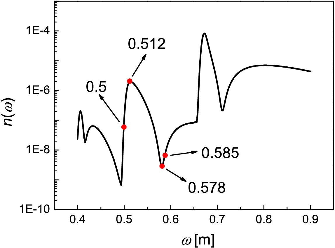
For Fig. 4 (a) where the laser frequency $\omega=0.5m$, when the laser frequency is not modulated, the number density of created particles is $1.04\times 10^{-7}$. While for $0\leq\alpha\leq 0.1$, the range of modulation parameters $(\omega_{m},b)$ is below the red dashed line, and the minimum and maximum values of the pair number density in this region are $A:1.04\times 10^{-7}$ and $B:2.00\times 10^{-6}$, respectively. It is found that the number density of created pairs corresponding to point $B$ is $20$ times greater than that without frequency modulation. For $0.1\leq\alpha\leq 0.32$, the range of modulation parameters is between the black dash-dot line and the red dashed line, and the minimum and maximum values of the particle number density in this region are $C:7.63\times 10^{-9}$ and $D:6.1\times 10^{-7}$, respectively. Although the maximum value of the number density corresponding to point $D$ is larger than that without frequency modulation, it is smaller than that corresponding to point $B$ where the modulation parameters belong to $0\leq\alpha\leq 0.1$. Moreover, the number density of created particles corresponding to point $C$ is even smaller than that without frequency modulation. This amazing result is caused by the same reason as the phenomenon occurring in Fig. 2, where the highest momentum peak does not always correspond to pair creation by absorbing the photons with dominant frequency component. To explain this result, we give the number density of created pairs varying with the field frequency, see Fig. 5. It can be seen that the pair number density is very sensitive to the field frequency. For example, the number density of created pairs by absorbing four photons with $\omega=0.512m$ is at least an order of magnitude greater than the one by absorbing four photons with $\omega=0.5m$. By analyzing the frequency spectra of the frequency modulated field at point $B$ (upper panel) and point $C$ (lower panel) shown in Fig. 6, we find that the dominant frequency components at point $B$ and $C$ are $0.512m$ and $0.578m$, which correspond to a peak and a valley of the particle number density shown in Fig. 5, respectively. Therefore, the pair number density at point $B$ is larger than the one without frequency modulation ($\omega=0.5m$), while the number density at point $C$ is smaller than the latter one. A similar result can also be found by comparing the values of momentum peaks in Figs. 2 (d), (a) and (f). Moreover, we know that the momentum peak $p_{18}$ in Fig. 2 (f) is formed by absorbing three photons with $\omega=0.578$ and one photon with $\omega=0.52$, and the number density for $\omega=0.52$ is much larger than that for $\omega=0.578$, so the value of momentum peak $p_{18}$ is higher than that of peak $p_{19}$, though the peak $p_{19}$ is formed by absorbing four photons with dominant frequency component. This analysis can also be used to understand momentum spectra in Figs. 2 (b) and (c), where highest peaks are not formed by absorbing four photons with dominant frequency component. By the way, when the modulation frequency at point $C$ changes from $0.01m$ to $0.009m$, one can see that the number density is also increased, see Fig. 4 (a), because the dominant frequency moves from $0.578m$ to $0.585m$ see Fig. 1 (b).

In the range of $0.32\leq\alpha\leq 1.0$, the minimum and maximum values of the number density of created pairs are $E:9.89\times 10^{-9}$ and $F:2.03\times 10^{-5}$, respectively. It can be seen that the number density at point $F$ is $200$ times greater than that without frequency modulation ($N=1.04\times 10^{-7}$). It is noticeable that the value of $\alpha$ is $0.38$ at point $F$, which the effective frequency belongs to a reasonable area. Since the maximum effective modulation frequency should not be larger than the original laser frequency, the modulation parameters in the range of $\alpha\geq 1.0$ have no actual meanings and are not discussed any more, although the number density of created particles is enhanced significantly in this region. Similar to Fig. 4 (a), the maximum value of the number density of created particles in Fig. 4 (b) is $L:3.50\times 10^{-4}$, which is also $200$ times greater than the number density without frequency modulation ($N=1.74\times 10^{-6}$). In this case, the value of $\alpha$ is $0.576$ at point $L$ and the effective frequency is still in a relatively reasonable area.

Based on the above discussion, we find that the number density of created pairs is not always enhanced by a frequency modulated field, but for certain modulation parameters it indeed can be increased significantly. Therefore, according to our theoretical analysis the particle number density may be enhanced by over two orders of magnitude by conducting the most basic and precise modulation of a laser beam experimentally. It should be noted that the reason why the enhancement effect of pair production for the frequency modulated field here is much weaker than that for a linear chirped field is because the largest effective frequency of the frequency modulated field is restricted to less than two times the original frequency.