跳到论文正文
W Papers独立论文阅读器 arXiv:1908.08065 论文正文 计算阅读时间 · 0%
引用这篇论文根据当前论文元数据生成,正式投稿前建议核对。


License: arXiv.org perpetual non-exclusive license
arXiv:1908.08065v1 [cond-mat.stat-mech] 21 Aug 2019

On a “continuum” formulation of the Ising model partition function

Francesco Caravelli E-mail: caravelli@lanl.gov Affiliation: Theoretical Division and Center for Nonlinear Studies,
Los Alamos National Laboratory, Los Alamos, New Mexico 87545, USA
Received: date / Accepted: date
Abstract

We derive an exact path integral formulation for the partition function for the Ising model using a mapping between spins and poles of a Laurent expansion for a field on the complex plane. The advantage in using this formulation for the evaluation of the partition function and n−n-point functions are twofold. First of all, we show that this mapping is independent of the couplings, and that for h=0h=0 it is possible to perform a low temperature expansion as a perturbation theory via Feynman diagrams. The couplings are mapped naturally to a propagator for a complex field. The combinatorial nature of the partition function is shown to lead to an auxiliary field with a non-zero external field interaction which enforces the spin-like nature. Feynman diagrams are shown to coincide with certain combinations of traces of coupling inverses in a certain rescaling.

Keywords: 
field theory, Ising model

1 Introduction

The question we ask ourselves in this paper is how to construct a field theory for the Ising model for arbitrary exchange interaction couplings, and without having to resort to a continuous limit. The continuum formulation of the partition function we provide has to be thought as a compact way of keeping track of indices contractions in a field theory of the Ising model, and as a mere mathematical curiosity on its own.

The Ising model is one of the oldest and most important models in Statistical Mechanics kittel; parisi; kadanoff; mussardo; baxter. The model is simple enough to have a large range of applicability and it can be solved exactly in one, two dimensions and infinite dimensions. Various real systems can be mapped to Ising models, including models of the gas-liquid transition baxter. In dimensions larger than four, the universality class is the same provided by the mean-field approximation. For the case in which there is a well established dimension and the couplings are all ferromagnetic, it is possible to derive a field theory as an expansion on the mean field. This is known as the Landau-Ginzburg model, and has been incredibly useful to study the order of phase transitions and via renormalization group, order dependent mapping zj or variational perturbation theory fk.

The starting point of this articles is the fact that a field theory for the Ising model is not known for arbitrary couplings, as far as we know. The key difficulty is the fact that the continuous limit of a discrete operator does not always converge to a well-known continuous counterpart as in the case of the discrete Laplacian on a regular lattice of DD-dimensions. The present paper proposes one formalism to overcome this difficulty, in part by hiding the discrete structure within a continuous operator, but without loosing the discrete nature of the model. This paper focuses on the formalism. In the next section we derive, with the use of the z-Transform, the mapping between the thermal field theory of the Ising model and an interacting field theory on the complex plane where the temperature is the perturbative parameter. The mathematical identity we use is simply based on Cauchy’s theorem for simple poles, and is a (rather simple) way of compactly performing indices contraction via (contour) integrations on the complex plane. We encode the spin-like nature of the Ising field in an auxiliary field via the introduction of of Dirac’s deltas in the path integration. As we will see, the auxiliary field does not have a quadratic term, and thus does not allow a perturbative expansion. In order to overcome this difficulty, we introduce a quadratic term by hand, and consider a particular rescaling of the mass with the temperature in which we can obtain the partition function via the resummation only of certain type of diagrams, in a Hartree-Fock fashion and for zero external field. In this spirit, the resummation is in the spirit of a double-scaling limit.

The interactions are then subsequently introduced, and peculiarity of the evaluation of the Feynman diagrams in this formalism described. The cases we study are in fact to elucidate the combinatorial properties of this field theory. We show that a certain choice of the countour integration can be thought of as a Group Field Theory Oriti.

2 Mapping on the complex plane

The Ising model has, despite its variety and richness in behavior, a simple Hamiltonian definition:

H=∑i​jJi​j​σi​σj+∑ihi​σi,H=\sum_{ij}J_{ij}\sigma_{i}\sigma_{j}+\sum_{i}h_{i}\sigma_{i},

where the variables σi=±1\sigma_{i}=\pm 1. Because of this, we can add an infinite constant to the Hamiltonian that can be reabsorbed into the diagonal Ji​i=miJ_{ii}=m_{i}, which contributes with Hd=∑imi​σi2=∑imiH_{d}=\sum_{i}m_{i}\sigma_{i}^{2}=\sum_{i}m_{i}. It is generally thought, however that it is not possible to write a consistent continuum theory when Jp​tJ_{pt} do not have some special symmetry, as for instance Euclidean, but in the following no assumption is made about the nature of the couplings Ji​jJ_{ij}.

2.1 Ising Hamiltonian as a continuous functional

The main technique we use is a rather simple integral transform commonly used to solve difference equations and for signal processing. We define the following transformation, called zz-Transform zt, which maps countable variables to a function on the complex plane:

χ⁡(z)\displaystyle\chi(z) =\displaystyle= ∑i=1nσj​z−j\displaystyle\sum_{i=1}^{n}\sigma_{j}z^{-j}
σj\displaystyle\sigma_{j} =\displaystyle= 12​π​i​∮𝒞d​z​χ​(z)​zj−1=12​π​i​∮𝒞d​zz​χ​(z)​zj\displaystyle\frac{1}{2\pi i}\oint_{\mathcal{C}}dz\chi(z)z^{j-1}=\frac{1}{2\pi i}\oint_{\mathcal{C}}\frac{dz}{z}\chi(z)z^{j} (1)

where we assume that the contour 𝒞\mathcal{C} contains the origin in the complex plane, and χ⁡(z):ℂ→ℂ\chi(z):\mathbb{C}\rightarrow\mathbb{C}. We see that the mapping above is based on Cauchy’s integral theorem. The function χ⁡(z)\chi(z) is not a smooth function in principle, as we do not require σj\sigma_{j} to fall off in the index jj in any reasonable fashion. Since we aim to use this transformation to obtain a path-integral over any possible (non-differentiable) function χ⁡(z)\chi(z), we do not see this as an obstruction. Some restriction will have however to be imposed on the coefficients σ\sigma later on. We can however see that eqn. (1) provides the right answer as the poles of n-th order behave as Kronecker delta functions, assuming that 𝒞\mathcal{C} is a contour that contains the origin in the complex plane. These formulae can be generalized by moving the origin and thus the contour somewhere else in the complex plane, but in what follows this generalization will be necessary later as we will have to explore. Let us now use this transformation on the Ising model. A quick calculation shows that the partition function becomes

Z\displaystyle Z =\displaystyle= ∑{σ}e−β∑i​jσiσjJi​j\displaystyle\sum_{\{\sigma\}}e^{-\beta\sum_{ij}\sigma_{i}\sigma_{j}J_{ij}} (2)
=\displaystyle= ∑{σ}e14​π2​β​∮𝒞∮𝒞d​z1​d​z2​χ​(z1)​χ​(z2)​∑i​jJi​j​z1i−1​z2j−1.\displaystyle\sum_{\{\sigma\}}e^{\frac{1}{4\pi^{2}}\beta\oint_{\mathcal{C}}\oint_{\mathcal{C}}dz_{1}dz_{2}\chi(z_{1})\chi(z_{2})\sum_{ij}J_{ij}z_{1}^{i-1}z_{2}^{j-1}}.

We note that χ⁡(1z)\chi(\frac{1}{z}) is a Taylor polynomial whose coefficients are the spin variables. The advantage of this transformation is that the summation can now be hidden in a continuous function, J⁡(z1−1,z2−1)≡∑i​jJi​j​z1i−1​z2j−1J(z_{1}^{-1},z_{2}^{-1})\equiv\sum_{ij}J_{ij}z_{1}^{i-1}z_{2}^{j-1}, which is close to the definition of 2-dimensional z-Transform where the variables have been inverted. It is not too difficult to show that the mapping provided by the z-Transform is a very compact way of performing matrix multiplication for discrete systems (e.g. where we can replace the index contraction with a complex integration).

In fact, it can be written as:

(z1​z2)−1​∑i​jJi​j​z1i​z2j≡(z1​z2)−1​J​(z1−1,z2−1)(z_{1}z_{2})^{-1}\sum_{ij}J_{ij}z_{1}^{i}z_{2}^{j}\equiv(z_{1}z_{2})^{-1}J(z_{1}^{-1},z_{2}^{-1}) (3)

where J⁡(z1,z2)=∑i​jJi​j​z1−i​z2−jJ(z_{1},z_{2})=\sum_{ij}J_{ij}z_{1}^{-i}z_{2}^{-j}. Thus, given a certain integration measure which we now describe, we now show that we can write the partition function as a functional integration over the field χ\chi:

Z\displaystyle Z =\displaystyle= ∫[D​χ​(z)]​P​(χ)​eβ4​π2​∮𝒞∮𝒞d​z1​d​z2z1​z2​χ​(z1)​χ​(z2)​J​(z1−1,z2−1).\displaystyle\int[D\chi(z)]P(\chi)e^{\frac{\beta}{4\pi^{2}}\oint_{\mathcal{C}}\oint_{\mathcal{C}}\frac{dz_{1}dz_{2}}{z_{1}z_{2}}\chi(z_{1})\chi(z_{2})J(z_{1}^{-1},z_{2}^{-1})}.

The external field term ∑ihi​σi=12​π​i​∮𝒞d​z​χ​(z)​∑ihi​zi−1\sum_{i}h_{i}\sigma_{i}=\frac{1}{2\pi i}\oint_{\mathcal{C}}dz\chi(z)\sum_{i}h_{i}z^{i-1} becomes

∑ihi​σi=12​π​i​∮𝒞d​zz​χ​(z)​h​(z−1).\sum_{i}h_{i}\sigma_{i}=\frac{1}{2\pi i}\oint_{\mathcal{C}}\frac{dz}{z}\chi(z)h(z^{-1}). (5)

Let us show that the functional we have written in eqn. (2) is correct, and poles do not interfere with each other. We have:

H\displaystyle H =\displaystyle= −1(2​π)2∮𝒞∮𝒞dz1dz2χ(z1)χ(z2)z1−1z2−1J(z1−1,z2−1)\displaystyle-\frac{1}{(2\pi)^{2}}\oint_{\mathcal{C}}\oint_{\mathcal{C}}dz_{1}dz_{2}\chi(z_{1})\chi(z_{2})z_{1}^{-1}z_{2}^{-1}J(z_{1}^{-1},z_{2}^{-1}) (6)
=\displaystyle= −1(2​π)2∑i​j∑q​t∮𝒞∮𝒞dz1dz2σiσjJq​tz1q−i−1z2t−j−1\displaystyle-\frac{1}{(2\pi)^{2}}\sum_{ij}\sum_{qt}\oint_{\mathcal{C}}\oint_{\mathcal{C}}dz_{1}dz_{2}\sigma_{i}\sigma_{j}J_{qt}z_{1}^{q-i-1}z_{2}^{t-j-1}
=\displaystyle= −1(2​π)2∑i​j∑q​tσiσjJq​t∮𝒞dz1z1−i+q−1∮𝒞dz2z2−j+t−1\displaystyle-\frac{1}{(2\pi)^{2}}\sum_{ij}\sum_{qt}\sigma_{i}\sigma_{j}J_{qt}\oint_{\mathcal{C}}dz_{1}z_{1}^{-i+q-1}\oint_{\mathcal{C}}dz_{2}z_{2}^{-j+t-1}
=\displaystyle= −1(2​π)2∑i​j∑q​tσiσjJq​t(−(2π)2)δi,qδj,t\displaystyle-\frac{1}{(2\pi)^{2}}\sum_{ij}\sum_{qt}\sigma_{i}\sigma_{j}J_{qt}\left(-(2\pi)^{2}\right)\delta_{i,q}\delta_{j,t}
=\displaystyle= ∑i​jσi​σj​Ji​j.\displaystyle\sum_{ij}\sigma_{i}\sigma_{j}J_{ij}.

The method can also be generalized to the case with interaction or n-body terms, which will be discussed elsewhere.

2.2 Scalar product and operator action

Before we discuss the path integral measure, it is worth explaining in a slightly more detailed fashion how the integral transform can be interpreted. It is obvious that the integral in eqn. (5) defines a scalar product between vectors, which is inherited from the fact that the functions were originally scalar products. We thus define

⟨f⁡(z),g⁡(z)⟩=12​π​i​∮𝒞d​zz​f​(z−1)​g​(z).\langle f(z),g(z)\rangle=\frac{1}{2\pi i}\oint_{\mathcal{C}}\frac{dz}{z}f(z^{-1})g(z). (7)

Albeit not obvious from the integral formula, the scalar product above is symmetric. The scalar product above will not be surprising for those familiar with Calogero-Sutherland-Moser models and Jack polynomials csm.

The integral operation of eqn. (7) can be extended also to the action of operators, which are defined as functions Q:ℂ×ℂ→ℂQ:\mathbb{C}\times\mathbb{C}\rightarrow\mathbb{C}. Let us write Q⁡(z1,z2)=∑i​jQi​j​zi​zjQ(z_{1},z_{2})=\sum_{ij}Q_{ij}z^{i}z^{j}. Given two operators Q1​(z1,z2)Q_{1}(z_{1},z_{2}) and Q2​(z1,z2)Q_{2}(z_{1},z_{2}), we define

(Q1∘Q2)​(z1,z2)=12​π​i​∮𝒞d​z​z−1​Q1​(z1,z−1)​Q2​(z,z2)(Q_{1}\circ Q_{2})(z_{1},z_{2})=\frac{1}{2\pi i}\oint_{\mathcal{C}}dz\ z^{-1}Q_{1}(z_{1},z^{-1})Q_{2}(z,z_{2}) (8)

which is easy to see it being is non-commutative. In fact, we have

(Q1CLOSE\displaystyle(Q_{1} ∘\displaystyle\circ OPENQ2)​(z1,z2)=12​π​i​∮𝒞Q1​(z1,z−1)​Q2​(z,z2)​z−1​𝑑z\displaystyle Q_{2})(z_{1},z_{2})=\frac{1}{2\pi i}\oint_{\mathcal{C}}Q_{1}(z_{1},z^{-1})Q_{2}(z,z_{2})z^{-1}dz (9)
=\displaystyle= 12​π​i​∑i​j,k​t∮𝒞(Q1)i​j​(Q2)k​t​z1i​zj​z−k,z2t​z−1​𝑑z\displaystyle\frac{1}{2\pi i}\sum_{ij,kt}\oint_{\mathcal{C}}(Q_{1})_{ij}(Q_{2})_{kt}z_{1}^{i}z^{j}z^{-k},z_{2}^{t}z^{-1}dz
=\displaystyle= 12​π​i​∑i​j,k​t∮𝒞(Q1)i​j​(Q2)k​t​z1i​zj−k+1​z2t​𝑑z\displaystyle\frac{1}{2\pi i}\sum_{ij,kt}\oint_{\mathcal{C}}(Q_{1})_{ij}(Q_{2})_{kt}z_{1}^{i}z^{j-k+1}z_{2}^{t}dz
=\displaystyle= ∑i​j,k​tQi​j​Qk​t​z1i​δj,k​z2t=∑i​t(∑k(Q1)i​k​(Q2)k​t)​z1i​z2t\displaystyle\sum_{ij,kt}Q_{ij}Q_{kt}z_{1}^{i}\delta_{j,k}z_{2}^{t}=\sum_{it}\left(\sum_{k}(Q_{1})_{ik}(Q_{2})_{kt}\right)z_{1}^{i}z_{2}^{t}
≡\displaystyle\equiv (Q1​Q2)​(z1,z2),\displaystyle(Q_{1}Q_{2})(z_{1},z_{2}),

from which we see that the operation inherits its non-commutativity from the standard matrix product. It does make sense to define for what follows the operation

[Q1∘⋯∘Qn](z1,z2)\displaystyle[Q_{1}\circ\cdots\circ Q_{n}](z_{1},z_{2}) =\displaystyle= 1(2​π​i)n∮𝒞⋯∮𝒞Q1(z1,z~1)⋯Qn−1(z~n−1,z2)∏i=1n−1d​z~iz~i\displaystyle\frac{1}{(2\pi i)^{n}}\oint_{\mathcal{C}}\cdots\oint_{\mathcal{C}}Q_{1}(z_{1},\tilde{z}_{1})\cdots Q_{n-1}(\tilde{z}_{n}^{-1},z_{2})\prod_{i=1}^{n-1}\frac{d\tilde{z}_{i}}{\tilde{z}_{i}} (10)

defined upon the matrix given by the matrix product Q=Q1Q2Q3⋯Qn−1Q=Q_{1}Q_{2}Q_{3}\cdots Q_{n-1}. This operation will turn to be useful later. The operation ∘\circ can be extended also to the action of the linear operator on a complex function, as

(J∘χ)​(z)=12​π​i​∮𝒞d​z~z~​J​(z,z~−1)​χ​(z~).(J\circ\chi)(z)=\frac{1}{2\pi i}\oint_{\mathcal{C}}\frac{d\tilde{z}}{\ \tilde{z}}J(z,\tilde{z}^{-1})\chi(\tilde{z}). (11)

Using the definition of the scalar product and the action of the linear operator on a function, the quadratic part of the Hamiltonian can be simply written as:

Hχ​χ=β⁡⟨χ⁡(z),(J∘χ)​(z)⟩.H_{\chi\chi}=\beta\langle\chi(z),(J\circ\chi)(z)\rangle. (12)

Thus, the Green function for the field χ\chi is simply provided by J−1​(z1,z2)J^{-1}(z_{1},z_{2}) defined using the inverse matrix Ji​j−1J_{ij}^{-1} if it exists, and is defined via the Cauchy integral operation. This result will be useful in perturbation theory as it defines the propagator.

2.3 A comment on the path integral measure

What is important is the measure of the path integral over the field χ⁡(z)\chi(z). First, we note that the sum over discrete spins can be written as ∑σi=2∫dσiδ(σi2−1)\sum_{\sigma_{i}}=2\int d\sigma_{i}\delta(\sigma_{i}^{2}-1) as it is well known. From the continuous variables σi\sigma_{i}, we can derive the measure above directly from the definition of the partition function (up to an irrelevant constant). In fact, we have d​χi≡d​χ​(zi)=∑jd​σj​zi−jd\chi_{i}\equiv d\chi(z_{i})=\sum_{j}d\sigma_{j}z_{i}^{-j}, from which it can be shown that, up to a Vandermonde determinant which is independent from the fields and which factors out, we can replace d​σid\sigma_{i} with [D​χ​(z)][D\chi(z)] up to a constant factor which depends on the embedding into the complex plane, but not on the fields. Let show the statement above with a little more care.

We distinguish the functional versus the normal delta functions Δ\Delta and δ\delta respectively, but the connection between the two should be obvious. But we are interested in writing the integration over [d​σ][d\sigma] as [d​χ​(z)][d\chi(z)]. This can be done via the introduction of a Jacobian, via the transformation: from which we obtain the Jacobian determinant:

[d​χ​(zi)]=|det​(∂χ⁡(z)∂σj)|​∏id​σj.[d\chi(z_{i})]=|\text{det}\left(\frac{\partial\chi(z)}{\partial\sigma_{j}}\right)|\prod_{i}d\sigma_{j}. (13)

We have that ∂χ⁡(zi)∂σj=zi−j\frac{\partial\chi(z_{i})}{\partial\sigma_{j}}=z_{i}^{-j} and thus it follows that the Jacobian is a Vandermonde determinant, given by M=det​(∂χ⁡(zi)∂σj)=∏p≠q(zp−zq)M=\text{det}(\frac{\partial\chi(z_{i})}{\partial\sigma_{j}})=\prod_{p\neq q}(z_{p}-z_{q}). While we have

[d​σ]=M−1​(z)​[d​χ​(z)],[d\sigma]=M^{-1}(z)[d\chi(z)], (14)

it is clear that the determinant function can be however reabsorbed as a field redefinition.11 1 Another way to see this, is by noticing that we now use the following integration over Grassmanian variables σi\sigma_{i} for the determinant of the matrix Mi​j=δi​j​zjM_{ij}=\delta_{ij}z^{j}: det(Mi​j)=∫∏i[dθi]e−∑iθiθizi.\text{det}(M_{ij})=\int\prod_{i}[d\theta_{i}]e^{-\sum_{i}\theta_{i}\theta_{i}z^{i}}. (15) The Grassmann field is however decoupled from the Hamiltonian reformulation.

2.4 Spin nature of the field

Insofar we have not achieved much as we still need to take care of the delta functions which provide the sum with the correct measure for the Ising model. We note that the summation in the partition function over the value of the spins in eqn. (2) can be written as a continuous integral as:

∑σi±1\displaystyle\sum_{\sigma_{i}\pm 1} =\displaystyle= ∏i∫d​σi​[δ⁡(σi−1)+δ⁡(σi+1)]\displaystyle\prod_{i}\int d\sigma_{i}[\delta(\sigma_{i}-1)+\delta(\sigma_{i}+1)] (16)
=\displaystyle= 2n​∏i∫d​σi​δ​(σi2−1)→∫[𝑑σ]​δ​(σ2​(x)−1).\displaystyle 2^{n}\prod_{i}\int d\sigma_{i}\delta(\sigma_{i}^{2}-1)\rightarrow\int[d\sigma]\delta(\sigma^{2}(x)-1).

The standard Landau-Ginzburg approach is to replace δ⁡(x)→e−γ​x2\delta(x)\rightarrow e^{-\gamma x^{2}}, and consider the action for large values of γ\gamma. Albeit possible, here we consider instead an auxiliary variable ηi\eta_{i}, and write δ⁡(σj2−1)∝∫d​ηj​ei​ηj​(σj2−1)\delta(\sigma_{j}^{2}-1)\propto\int d\eta_{j}e^{i\eta_{j}(\sigma_{j}^{2}-1)}, simply because this is exact. For consistency with what follows, we introduce the notion of Cauchy delta function, δC​(z−z0)=12​π​i​1z−z0\delta_{C}(z-z_{0})=\frac{1}{2\pi i}\frac{1}{z-z_{0}}, such that ∮𝒞d​z​f​(z)​δC​(z−z0)=f⁡(z0)\oint_{\mathcal{C}}dzf(z)\delta_{C}(z-z_{0})=f(z_{0}).

Using the z-Transform again, we obtain:

−i∑kηk\displaystyle-i\sum_{k}\eta_{k} =\displaystyle= −∮𝒞z−1η(z)δC(z−1)dz\displaystyle-\oint_{\mathcal{C}}z^{-1}\eta(z)\delta_{C}(z-1)dz
i​∑kηk​σk​σk\displaystyle i\sum_{k}\eta_{k}\sigma_{k}\sigma_{k} =\displaystyle= −i4​π2∮𝒞∮𝒞d​z1​d​z2z1​z2η(z1−1z2−1)χ(z1)χ(z2)\displaystyle-\frac{i}{4\pi^{2}}\oint_{\mathcal{C}}\oint_{\mathcal{C}}\frac{dz_{1}dz_{2}}{z_{1}z_{2}}\eta(z_{1}^{-1}z_{2}^{-1})\chi(z_{1})\chi(z_{2})

with η⁡(z)=∑kηk​z−k\eta(z)=\sum_{k}\eta_{k}z^{-k}. Thus, using the z-Transform above we identify the seemingly innocuous −i∑kηk-i\sum_{k}\eta_{k} as an external field interaction with the auxiliary field δC​(z)\delta_{C}(z). From the point of view of a perturbative expansion for the path integral, it is interesting to note that the field η\eta does not have any quadratic term, which is something we will have to deal with later. We thus introduce this regularization rather artificially in the Hamiltonian, as

Hη​η\displaystyle H_{\eta\eta} =\displaystyle= −m24​π2∮𝒞η⁡(z)​η​(z−1)2z−1dz,\displaystyle-\frac{m^{2}}{4\pi^{2}}\oint_{\mathcal{C}}\frac{\eta(z)\eta(z^{-1})}{2}z^{-1}dz, (17)

with the purpose of studying perturbations theory. A suitable way of doing the limit m→0m\rightarrow 0 has, however, to be devised. If we consider all the terms together, we find the following partition function for the Ising model:

Z\displaystyle Z =\displaystyle= ∫[Dχ(z)][Dη(z)]e−∮𝒞dzz−1η(z)δ(z−1)+14​π2∮𝒞∮𝒞dz1dz2χ(z1)χ(z2)z1−1z2−1(−iη(z1−1z2−1)+βJ(z1−1,z2−1))\displaystyle\int[D\chi(z)][D\eta(z)]e^{-\oint_{\mathcal{C}}dzz^{-1}\eta(z)\delta(z-1)+\frac{1}{4\pi^{2}}\oint_{\mathcal{C}}\oint_{\mathcal{C}}dz_{1}dz_{2}\chi(z_{1})\chi(z_{2})z_{1}^{-1}z_{2}^{-1}\left(-i\eta(z_{1}^{-1}z_{2}^{-1})+\beta J(z_{1}^{-1},z_{2}^{-1})\right)} (18)
⋅\displaystyle\cdot e−iβ12​π∮𝒞dz1z1−1χ(z1)h(z1−1)−m24​π2∮𝒞η⁡(z)​η​(z−1)2z−1dz,\displaystyle e^{-i\beta\frac{1}{2\pi}\oint_{\mathcal{C}}dz_{1}z_{1}^{-1}\chi(z_{1})h(z_{1}^{-1})-\frac{m^{2}}{4\pi^{2}}\oint_{\mathcal{C}}\frac{\eta(z)\eta(z^{-1})}{2}z^{-1}dz},

in which we have two interacting fields η\eta and χ\chi. The path integral above is one of the key results of this paper, and which we will now study. The path integral is equivalent to the Ising model in the limit m→0m\rightarrow 0, but as mentioned we do not require to have any other scale going to zero. We also note that the Hamiltonian is quadratic in χ\chi. There is an interaction term χ​χ​η\chi\chi\eta, together with the external field interaction of η\eta, enforces the spin-like origin of the field χ\chi, which makes the model non-trivial. At a first sight, we might wonder why the Landau-Ginzburg Hamiltonian is the truncated, continuum version of an Ising model, meanwhile the Hamiltonian above is quadratic. Clearly, the quadratic nature of the energy described by eqn. (18) is only an illusion, and the interaction with χ\chi generates an infinite tower of effective vertices for the field η\eta. In fact, interacting quadratic field theories, with cubic interactions and with a complex interaction constant are the intermediate field representation of a ϕ4\phi^{4} scalar field theory. Also, since at the bare level the η\eta field does not technically propagate, it cannot be interpreted as a fractionalization of a ϕ4\phi^{4} theory unless we introduce a mass term. We will discuss this later in this paper. Also, if 𝒞\mathcal{C} is chosen to be the unit circle, we note that any polynomial function defined on the unit circle will satisfy the property χ⁡(z−1)=χ∗​(z)\chi(z^{-1})=\chi^{*}(z) if the coefficients are real. In this case, the partition function that we have introduced is exactly a particular Group Field Theory on the unitary group with a non-trivial propagator for the field χ⁡(z)\chi(z) Oriti.

What can be evaluated using the partition function above are general correlators of the form

GN(z1,⋯,zN)=⟨χ(z1)⋯χ(zN)⟩,G_{N}(z_{1},\cdots,z_{N})=\langle\chi(z_{1})\cdots\chi(z_{N})\rangle, (19)

from which we can obtain information on the spins from an inverse z-Transform. Intermediate calculations can be done via various methods, perturbative or non-perturbative, via the accumulated knowledge obtained in field theory.

2.5 Where are the dimensions?

What might seem suspicious of the mapping above is that we have mapped any notion of dimensionality into a one dimensional one. Such impression is only superficial. The notion of dimensionality is not necessarily connected to the dimension of the embedding of the field, but rather to the notion of locality of the quadratic form associated with the propagator. In this sense, we have traded low dimensionality with locality, and the z-Transform mapping is not necessarily a simplification but a reformulation that demands to be studied. For certain systems, the infinite sum contained in the operator J⁡(z1,z2)J(z_{1},z_{2}) can be done explicitly. In fact, in those cases where dimensionality is well known, the function J⁡(z1,z2)J(z_{1},z_{2}) can be calculated exactly. Consider for instance the case of the one dimensional Ising model, Ji​j=J0​(δi,j+1+δi+1,j)J_{ij}=J_{0}(\delta_{i,j+1}+\delta_{i+1,j}). The transformed polynomial is given by:

J~​(z1,z2)=∑i​j∞δi,j+1​z1i​z2j=−J02​z1+z21−z1​z2\tilde{J}(z_{1},z_{2})=\sum_{ij}^{\infty}\delta_{i,j+1}z_{1}^{i}z_{2}^{j}=-\frac{J_{0}}{2}\frac{z_{1}+z_{2}}{1-z_{1}z_{2}} (20)

Analogously, the field χ⁡(z)→χ⁡(x→)\chi(z)\rightarrow\chi(\vec{x}) becomes

σi1,⋯,iD=1(2​π​i)D∮𝒞⋯∮𝒞χ(z1,⋯,zD)∏ν=1Dzνiνdzν\sigma_{i_{1},\cdots,i_{D}}=\frac{1}{(2\pi i)^{D}}\oint_{\mathcal{C}}\cdots\oint_{\mathcal{C}}\chi(z_{1},\cdots,z_{D})\prod_{\nu=1}^{D}z_{\nu}^{i_{\nu}}dz_{\nu} (21)

with

χ⁡(z→∈ℂD)=∑i1,⋯,inσi1,⋯,in​∏k=1Dzk−ik−1.\chi(\vec{z}\in\mathbb{C}^{D})=\sum_{i_{1},\cdots,i_{n}}\sigma_{i_{1},\cdots,i_{n}}\prod_{k=1}^{D}z_{k}^{-i_{k}-1}.

Using the Fourier transform for lattices, we can obtain a formula for the matrix Jk​lJ_{kl} and its inverse, as

Jk​l\displaystyle J_{kl} =\displaystyle= 1(2​π)D​∫ℬdD​p​G​(p)​ei⁡(k→−l→)⋅p→\displaystyle\frac{1}{(2\pi)^{D}}\int_{\mathcal{B}}d^{D}pG(p)e^{i(\vec{k}-\vec{l})\cdot\vec{p}}
G⁡(p)\displaystyle G(p) =\displaystyle= ϵ−2​J​∑ν=1Dcos⁡(pν)\displaystyle\epsilon-2J\sum_{\nu=1}^{D}\cos(p_{\nu}) (22)

and thus obtain the exact inverse in the Fourier representation:

J⁡(z→1,z→2)\displaystyle J(\vec{z}_{1},\vec{z}_{2}) =\displaystyle= ∫ℬdD​p(2​π)D​G⁡(p→)∏ν=1D(1−ei​pν​z1​ν)ei​pν​z1​ν​(1−e−i​pν​z2​ν)e−i​pν​z2​ν\displaystyle\int_{\mathcal{B}}\frac{d^{D}p}{(2\pi)^{D}}\frac{G(\vec{p})}{\prod_{\nu=1}^{D}\frac{(1-e^{ip_{\nu}}z_{1\nu})}{e^{ip_{\nu}}z_{1\nu}}\frac{(1-e^{-ip_{\nu}}z_{2\nu})}{e^{-ip_{\nu}}z_{2\nu}}}

where z→i=(zi​1,⋯,zi​d)\vec{z}_{i}=(z_{i1},\cdots,z_{id}). Also, the formulae above provide an exact representation for the trace. Since Trace​(J⁡(z1,z2))=12​π​i​∮𝒞d​zz​J​(z,z−1)=∑iJi​i\text{Trace}\left(J(z_{1},z_{2})\right)=\frac{1}{2\pi i}\oint_{\mathcal{C}}\frac{dz}{z}J(z,z^{-1})=\sum_{i}J_{ii}, we have simply

Tr​(J−1)=1(2​π)D​∫ℬdD​p​G−1​(p),\text{Tr}\left(J^{-1}\right)=\frac{1}{(2\pi)^{D}}\int_{\mathcal{B}}d^{D}p\ G^{-1}(p),

as one would expect. We have checked that the cofficients were right by direct inspection of all the possible Wick contractions.

It is also easy to see that we can define the Fourier transform of a function as:

χ~​(p)\displaystyle\tilde{\chi}(p) =\displaystyle= 12​π​i​∮𝒞d​zz−1​χ​(z−1)​ei​p​zei​p​z−1\displaystyle\frac{1}{2\pi i}\oint_{\mathcal{C}}\frac{dz}{z^{-1}}\chi(z^{-1})\frac{e^{ip}z}{e^{ip}z-1}
χ⁡(z)\displaystyle\chi(z) =\displaystyle= 12​π​∫−πaπad​p​e−i​p​ze−i​p​z−1​χ~​(p).\displaystyle\frac{1}{2\pi}\int_{-\frac{\pi}{a}}^{\frac{\pi}{a}}dp\frac{e^{-ip}z}{e^{-ip}z-1}\tilde{\chi}(p). (24)

The transforms above can be easily be generalized to DD dimensions via the introduction of a z-Transform for every index of the field σi1,⋯,iD\sigma_{i_{1},\cdots,i_{D}}.

3 Some trivial cases

Let us discuss now a couple of simple cases where we can show that the path integral does indeed provide a connection between spin models and interacting scalar fields on the complex plane.

The fact that the path integral seems to be so simple does not mean that the approach above is simpler than other exact methods. For instance, we could not recover insofar any known results on 1-dimensional or 2-dimensional ferromagnetic models. This is due to the fact that we replaced the spin-like nature of the system with a scalar Yukawa interaction, which generates an infinite tower of interactions. In part, this is due to the fact that if we could solve the approach above exactly, we would solve any Ising model. Here we discuss two trivial cases in this formalism.

3.1 Case m=0m=0, J=0J=0, h≠0h\neq 0

This case is rather trivial, but it will help in boosting the confidence that the field theory we introduce does correspond to a spin model. In the case J=0J=0, if the approach above is correct, we should be able to recover the standard Z=∏cosh⁡(β​h)Z=\prod\cosh(\beta h). This case is sufficiently non-trivial in the approach we propose that requires a section on its own. Let us first work out the case of a single spin. This will enlighten the fact that, albeit with some care, the integral over η\eta and σ\sigma can be inverted. We have:

∑σ±1e−β​σ​h=2​cosh⁡(β​h)\sum_{\sigma\pm 1}e^{-\beta\sigma h}=2\cosh(\beta h) (25)

We write:

∑σ±1e−β​σ​h\displaystyle\sum_{\sigma\pm 1}e^{-\beta\sigma h} =\displaystyle= 2​∫−∞∞d​σ​δ​(σ2−1)​e−β​σ​h=1π​∫−∞∞d​σ​∫−∞∞d​η​ei⁡(σ2−1)​η−β​σ​h\displaystyle 2\int_{-\infty}^{\infty}d\sigma\delta(\sigma^{2}-1)e^{-\beta\sigma h}=\frac{1}{\pi}\int_{-\infty}^{\infty}d\sigma\int_{-\infty}^{\infty}d\eta\ e^{i(\sigma^{2}-1)\eta-\beta\sigma h} (26)

We now invert the order of the integration:

Z\displaystyle Z =\displaystyle= 1π​∫−∞∞d​σ​∫−∞∞d​η​ei⁡(σ2−1)​η−β​σ​h\displaystyle\frac{1}{\pi}\int_{-\infty}^{\infty}d\sigma\int_{-\infty}^{\infty}d\eta\ e^{i(\sigma^{2}-1)\eta-\beta\sigma h} (27)
=\displaystyle= 1π​∫−∞∞d​η​∫−∞∞d​σ​ei⁡(σ2−1)​η−β​σ​h\displaystyle\frac{1}{\pi}\int_{-\infty}^{\infty}d\eta\int_{-\infty}^{\infty}d\sigma\ e^{i(\sigma^{2}-1)\eta-\beta\sigma h}
=\displaystyle= 1π​∫−∞∞d​η​π​ei​β2​h24​η−i​η−i​η\displaystyle\frac{1}{\pi}\int_{-\infty}^{\infty}d\eta\frac{\sqrt{\pi}e^{\frac{i\beta^{2}h^{2}}{4\eta}-i\eta}}{\sqrt{-i\eta}}

We now perform the following Wick rotation: η→i​η\eta\rightarrow i\eta, and obtain

Z=−2π2​π​i∫−i​∞i​∞dηeη+β2​h24​ηηZ=-2\frac{\sqrt{\pi}}{2\pi i}\int_{-i\infty}^{i\infty}d\eta\frac{e^{\eta+\frac{\beta^{2}h^{2}}{4\eta}}}{\sqrt{\eta}} (28)

and, as it turns out, the integral above is a representation of the hyperbolic cosine function ris:

π2​π​i​∫ϵ−i​∞ϵ+i​∞d​η​eη+β2​h24​ηη=cosh⁡(β​h),\frac{\sqrt{\pi}}{2\pi i}\int_{\epsilon-i\infty}^{\epsilon+i\infty}d\eta\frac{e^{\eta+\frac{\beta^{2}h^{2}}{4\eta}}}{\sqrt{\eta}}=\cosh(\beta h),

for ϵ>0\epsilon>0. We thus recover the same result.

Let us now discuss the case with multiple non-interacting spins. We use the integration we have performed before. We have

Z\displaystyle Z =\displaystyle= ∫[Dχ(z)][Dη(z)]e−∮𝒞dzz−1η(z)δ(z−1)e−i4​π2∮𝒞∮𝒞dz1dz2χ(z1)χ(z2)z1−1z2−2η(z1−1z2−1)\displaystyle\int[D\chi(z)][D\eta(z)]e^{-\oint_{\mathcal{C}}dzz^{-1}\eta(z)\delta(z-1)}e^{-\frac{i}{4\pi^{2}}\oint_{\mathcal{C}}\oint_{\mathcal{C}}dz_{1}dz_{2}\chi(z_{1})\chi(z_{2})z_{1}^{-1}z_{2}^{-2}\eta(z_{1}^{-1}z_{2}^{-1})}
⋅\displaystyle\cdot e−iβ12​π∮𝒞dz1z1−1χ(z1)h(z1−1)\displaystyle e^{-i\beta\frac{1}{2\pi}\oint_{\mathcal{C}}dz_{1}z_{1}^{-1}\chi(z_{1})h(z_{1}^{-1})}
=\displaystyle= ∫[Dη(z)]Q(η)e−∮𝒞dzz−1η(z)δ(z−1)ei​β2​∮𝒞∮𝒞d​z1​d​z2​z1−1​z2−1​h⁡(z1−1)​h​(z2−1)4​A​(z1,z2)−1\displaystyle\int[D\eta(z)]Q(\eta)e^{-\oint_{\mathcal{C}}dzz^{-1}\eta(z)\delta(z-1)}e^{i\beta^{2}\oint_{\mathcal{C}}\oint_{\mathcal{C}}dz_{1}dz_{2}z_{1}^{-1}z_{2}^{-1}\frac{h(z_{1}^{-1})h(z_{2}^{-1})}{4}A(z_{1},z_{2})^{-1}}

where A⁡(z1−1​z2−1)=η​(z)−1​δ​(z−z1−1​z2−1)A(z_{1}^{-1}z_{2}^{-1})=\eta(z)^{-1}\delta(z-z_{1}^{-1}z_{2}^{-1}) and Q⁡(η)=C(−i)n​det​(η⁡(z1−1​z2−1))Q(\eta)=\frac{C}{\sqrt{(-i)^{n}\text{det}(\eta(z_{1}^{-1}z_{2}^{-1}))}} with CC an integration constant. We note that the (functional) inverse of a function A⁡(x,y)A(x,y) is such that ∫d​z​A​(x,z)​A−1​(z,y)=δ⁡(x−y)\int dzA(x,z)A^{-1}(z,y)=\delta(x-y). In this sense, the Dirac delta function is its own inverse, as ∫d​z​δ​(x−z)​δ​(z−y)=δ⁡(x−y)\int dz\delta(x-z)\delta(z-y)=\delta(x-y). Thus, A​(z1,z2)−1=η​(z)−1​δ​(z−z1−1​z2−1)A(z_{1},z_{2})^{-1}=\eta(z)^{-1}\delta(z-z_{1}^{-1}z_{2}^{-1}). We now use the discretization of the function η⁡(z1,z2)=η⁡(zi,zj)=∑kηk​ei⁡(θi+θj)​(k−1)\eta(z_{1},z_{2})=\eta(z_{i},z_{j})=\sum_{k}\eta_{k}e^{i(\theta_{i}+\theta_{j})(k-1)}. This is the product of three matrices. In fact we can write

η⁡(zk,zt)=∑p​qei​θk​p​δp​q​ηp​ei​θj​q=(M​diag​(ηi)​Mt)k​t\eta(z_{k},z_{t})=\sum_{pq}e^{i\theta_{k}p}\delta_{pq}\eta_{p}e^{i\theta_{j}q}=(M\text{diag}(\eta_{i})M^{t})_{kt} (29)

where Mk​t=ei​θk​(t−1)M_{kt}=e^{i\theta_{k}(t-1)}. Thus det​(η⁡(zi,zj))=det2​(M)​det​((d​i​a​g​(η))=det2​(M)​∏iηiCLOSE\text{det}(\eta(z_{i},z_{j}))=\text{det}^{2}(M)\text{det}((diag(\eta))=\text{det}^{2}(M)\prod_{i}\eta_{i}. We choose a discretization of the z variables along the circle such that it matches that number of components in ηi\eta_{i}, σi\sigma_{i} and hih_{i}, and take the joint continuum limit N→∞N\rightarrow\infty. As such, also the inverse operator can be written as

η​(zk−1,zt−1)−1=∑rMk​r−t​ηr−1​Mr​t−1\eta(z_{k}^{-1},z_{t}^{-1})^{-1}=\sum_{r}M^{-t}_{kr}\eta_{r}^{-1}M^{-1}_{rt} (30)

We now have that the matrix MM is a DFT transformation with ω=ei​2​πN\omega=e^{i\frac{2\pi}{N}}. Its inverse simply requires the change of sign at the exponent. Thus, in order to calculate the inverse, we show that

Qk,r\displaystyle Q_{k,r} =\displaystyle= ∑pei​θk​t​e−i​θt​r=∑k,rei​2​πN​k​t−i​2​πN​t​r\displaystyle\sum_{p}e^{i\theta_{k}t}e^{-i\theta_{t}r}=\sum_{k,r}e^{i\frac{2\pi}{N}kt-i\frac{2\pi}{N}tr} (31)
=\displaystyle= ∑te−i​2​πN​t​(k−r)={0 if ​k≠rN if ​k=r\displaystyle\sum_{t}e^{-i\frac{2\pi}{N}t(k-r)}=\begin{cases}0&\text{ if }k\neq r\\ N&\text{ if }k=r\end{cases}

which is non-zero only if k=rk=r. We do not have to go through the discretization, however. In the continuum, the operator η−1​(z1−1,z2−1)\eta^{-1}(z_{1}^{-1},z_{2}^{-1}) can be obtained from the ansatz η−1​(z1−1,z2−1)=c​∑k2ηk2−1​e−i⁡(θ1+θ2)​k2\eta^{-1}(z_{1}^{-1},z_{2}^{-1})=c\sum_{k_{2}}\eta_{k_{2}}^{-1}e^{-i(\theta_{1}+\theta_{2})k_{2}}, for a certain constant cc, which has to satisfy

⟨η,η−1⟩\displaystyle\langle\eta,\eta^{-1}\rangle =\displaystyle= ∮d​z2​z2−1​η​(z1−1,z2−1)​η−1​(z2−1,z3−1)\displaystyle\oint dz_{2}z_{2}^{-1}\eta(z_{1}^{-1},z_{2}^{-1})\eta^{-1}(z_{2}^{-1},z_{3}^{-1}) (32)
=\displaystyle= −i∫02​πdθ2c∑k1,k2ηk1ηk2ei⁡(θ1+θ2)​k1−i⁡(θ2+θ3)​k2\displaystyle-i\int_{0}^{2\pi}d\theta_{2}c\sum_{k_{1},k_{2}}\frac{\eta_{k_{1}}}{\eta_{k_{2}}}e^{i(\theta_{1}+\theta_{2})k_{1}-i(\theta_{2}+\theta_{3})k_{2}}
=\displaystyle= δ⁡(θ1−θ2)\displaystyle\delta(\theta_{1}-\theta_{2})

We now observe that ∫02​πdθ2​ei​θ2​(k1−k2)=−2​π​i​δk1,k2\int_{0}^{2\pi}d_{\theta_{2}}e^{i\theta_{2}(k_{1}-k_{2})}=-2\pi i\delta_{k_{1},k_{2}}. From which we obtain

∮d​z2​z2−1​η​(z1−1,z2−1)​η−1​(z2−1,z3−1)\displaystyle\oint dz_{2}\ z_{2}^{-1}\eta(z_{1}^{-1},z_{2}^{-1})\eta^{-1}(z_{2}^{-1},z_{3}^{-1}) =\displaystyle= 2​π​∑kei⁡(θ1−θ3)​k\displaystyle 2\pi\sum_{k}e^{i(\theta_{1}-\theta_{3})k} (33)
=\displaystyle= 2​π​δ​(θ1−θ3)\displaystyle 2\pi\delta(\theta_{1}-\theta_{3})

Thus, we can set c=12​πc=\frac{1}{2\pi}. The term off-diagonal terms are zero as the elements are roots of unity. A quick calculation shows that the integration over z1z_{1} and z2z_{2} can be performed, and thus

F⁡(h,h)\displaystyle F(h,h) =\displaystyle= ∮𝒞∮𝒞d​z1​d​z2​z1−1​z2−1​h⁡(z1−1)​h​(z2−1)4​A​(z1,z2)−1\displaystyle\oint_{\mathcal{C}}\oint_{\mathcal{C}}dz_{1}dz_{2}z_{1}^{-1}z_{2}^{-1}\frac{h(z_{1}^{-1})h(z_{2}^{-1})}{4}A(z_{1},z_{2})^{-1} (34)
=\displaystyle= ∫02​π∫02​πd​θ1​d​θ2​hi​hjηk​ei​θ1​(i−k)​ei​θ1​(j−k)\displaystyle\int_{0}^{2\pi}\int_{0}^{2\pi}d\theta_{1}d\theta_{2}\frac{h_{i}h_{j}}{\eta_{k}}e^{i\theta_{1}(i-k)}e^{i\theta_{1}(j-k)}

from which we evince that the only surviving term is the one wih i=j=ki=j=k and gives a factor

∮𝒞∮𝒞d​z1​d​z2​z1−1​z2−1​h⁡(z1−1)​h​(z2−1)4​A​(z1,z2)−1=∑ihi24​ηi\oint_{\mathcal{C}}\oint_{\mathcal{C}}dz_{1}dz_{2}z_{1}^{-1}z_{2}^{-1}\frac{h(z_{1}^{-1})h(z_{2}^{-1})}{4}A(z_{1},z_{2})^{-1}=\sum_{i}\frac{h_{i}^{2}}{4\eta_{i}} (35)

We thus obtain, using the result on the single spin obtained in the previous section, by means of ηk→−i​ηk\eta_{k}\rightarrow-i\eta_{k}, that

Z∝∏icosh⁡(β​hi),Z\propto\prod_{i}\cosh(\beta h_{i}), (36)

which is the same result up to an external field redefinition. This shows the correctness of the functional approach above.

3.2 No constraints: the case without auxiliary field and generalization

It is clear that the auxiliary field imposes the constraint on the path integral to sum over functions which have only terms in the Laurent expansion which take a finite number of values. If σ\sigma’s are free to be chosen over the real line, then the partition function does not require an auxiliary field η\eta and the model is equivalent to the Gaussian one parisi. In this specific case, the partition function integration should read:

Z\displaystyle Z =\displaystyle= ∫[D​χ​(z)]​eβ4​π2​∮𝒞∮𝒞d​z1​d​z2​χ​(z1)​χ​(z2)​z1−1​z2−2​J​(z1−1,z2−1)−i​β​12​π​∮𝒞d​z1​z1−1​χ​(z1)​h​(z1−1)\displaystyle\int[D\chi(z)]e^{\frac{\beta}{4\pi^{2}}\oint_{\mathcal{C}}\oint_{\mathcal{C}}dz_{1}dz_{2}\chi(z_{1})\chi(z_{2})z_{1}^{-1}z_{2}^{-2}J(z_{1}^{-1},z_{2}^{-1})-i\beta\frac{1}{2\pi}\oint_{\mathcal{C}}dz_{1}z_{1}^{-1}\chi(z_{1})h(z_{1}^{-1})} (37)
∝\displaystyle\propto 1det​(J~​(z1,z2))​eξ2​β2(i​2​π)2​4​π2β​∮𝒞∮𝒞d​z1​d​z2​z1−1​z2−2​h​(z1−1)​h​(z2−1)​J~−1​(z1,z2).\displaystyle\frac{1}{\sqrt{\text{det}(\tilde{J}(z_{1},z_{2}))}}e^{\frac{\xi}{2}\frac{\beta^{2}}{(i2\pi)^{2}}\frac{4\pi^{2}}{\beta}\oint_{\mathcal{C}}\oint_{\mathcal{C}}dz_{1}dz_{2}z_{1}^{-1}z_{2}^{-2}h(z_{1}^{-1})h(z_{2}^{-1})\tilde{J}^{-1}(z_{1},z_{2})}.

The constant ξ\xi can be fixed by the knowledge of the exact integral in the starting case, as we can write

Z⁡(h→)\displaystyle Z(\vec{h}) =\displaystyle= ∫−∞∞dσie−β∑i​jJi​jσiσj−β∑ihiσi=2​πndet​(β​J)eβ2​∑i​jhi​hj​Ji​j−1.\displaystyle\int_{-\infty}^{\infty}d\sigma_{i}e^{-\beta\sum_{ij}J_{ij}\sigma_{i}\sigma_{j}-\beta\sum_{i}h_{i}\sigma_{i}}=\frac{\sqrt{2\pi}^{n}}{\sqrt{\text{det}(\beta J)}}e^{\frac{\beta}{2}\sum_{ij}h_{i}h_{j}J_{ij}^{-1}}. (38)

We thus need to convince ourselves that ∮𝒞∮𝒞d​z1​d​z2​z1−1​z2−2​h​(z1−1)​h​(z2−1)​J~−1​(z1,z2)∝∑i​jhi​hj​Ji​j−1\oint_{\mathcal{C}}\oint_{\mathcal{C}}dz_{1}dz_{2}z_{1}^{-1}z_{2}^{-2}h(z_{1}^{-1})h(z_{2}^{-1})\tilde{J}^{-1}(z_{1},z_{2})\propto\sum_{ij}h_{i}h_{j}J_{ij}^{-1}. Using the result on the inverse operator from the previous sections, it is straightforward to note that we can fix ξ=i2​π\xi=\frac{i}{2\pi}. We have

Z\displaystyle Z =\displaystyle= ∫[Dχ(z)]eβ4​π2​∮𝒞∮𝒞d​z1​d​z2​χ​(z1)​χ​(z2)​z1−1​z2−2​J​(z1−1,z2−1)e−iβ12​π∮𝒞dz1z1−1χ(z1)h(z1−1)\displaystyle\int[D\chi(z)]e^{\frac{\beta}{4\pi^{2}}\oint_{\mathcal{C}}\oint_{\mathcal{C}}dz_{1}dz_{2}\chi(z_{1})\chi(z_{2})z_{1}^{-1}z_{2}^{-2}J(z_{1}^{-1},z_{2}^{-1})}e^{-i\beta\frac{1}{2\pi}\oint_{\mathcal{C}}dz_{1}z_{1}^{-1}\chi(z_{1})h(z_{1}^{-1})}
=\displaystyle= eβ4​π​i​∮𝒞∮𝒞d​z1​d​z2​z1−1​z2−2​h​(z1−1)​h​(z2−1)​J~−1​(z1,z2)det​(J~​(z1,z2)).\displaystyle\frac{e^{\frac{\beta}{4\pi i}\oint_{\mathcal{C}}\oint_{\mathcal{C}}dz_{1}dz_{2}z_{1}^{-1}z_{2}^{-2}h(z_{1}^{-1})h(z_{2}^{-1})\tilde{J}^{-1}(z_{1},z_{2})}}{\sqrt{\text{det}(\tilde{J}(z_{1},z_{2}))}}.

From the analysis above, we can also see for instance that

1β​δ​h​(z1−1)​1β​δ​h​(z2−1)​Z=𝔼⁡[χ⁡(z1)​χ​(z2)]=1β​J−1​(z1,z2)\frac{1}{\beta\delta h(z_{1}^{-1})}\frac{1}{\beta\delta h(z_{2}^{-1})}Z=\mathbb{E}[\chi(z_{1})\chi(z_{2})]=\frac{1}{\beta}J^{-1}(z_{1},z_{2}) (40)

from which we obtain the result that the continuous spin correlator.

4 Interactions

4.1 Field rescaling for perturbation theory

The path integral formulation we obtained above is completely equivalent to the partition function of the Ising model, and in fact it has to be thought not as a novelty, but as a compact way to keep track of the indices contractions. In fact, it goes without saying that one could introduce the integral for each spin, the auxiliary spins, and use this field theory, as it is usually done in thermal field theory. However, we have found some peculiarities of this formalism novel enough to write a paper on its own on the subject.

We now discuss how to use the field theory in the complex plane we discussed using perturbation theory. The perturbative coupling constant, which is the inverse temperature, is in fact on the propagator. In order to perform the perturbative expansion however, we need to move the coupling to the interaction term. Thus, we consider the rescaled fields χ→1β​χ\chi\rightarrow\sqrt{\frac{1}{\beta}}\chi, and we consider h⁡(z)=0h(z)=0 for simplicity. Then, the propagator term for χ\chi looses β\beta, while the term χ​χ​η\chi\chi\eta acquires a coupling constant g=TJg=\frac{T}{J} which we can use for a perturbation theory.

Here we make a comment about how to interpret a perturbative expansion of the interaction term χ​χ​η\chi\chi\eta at h=0h=0. In principle the expansion is well defined for β\beta finite, and if the propagator J⁡(z1,z2)J(z_{1},z_{2}) is positive. We can add a diagonal term to the interaction, equivalent to an infinite constant, −nm2=−m2∑iσi2-nm^{2}=-m^{2}\sum_{i}\sigma_{i}^{2}, and use mm as a regularization of the integrals. The quadratic term thus becomes of the form −m2​δi​j+β​Ji​j→−m2​z1​z2(1−z1​z2)+β​J​(z1,z2)-m^{2}\delta_{ij}+\beta J_{ij}\rightarrow-m^{2}\frac{z_{1}z_{2}}{(1-z_{1}z_{2})}+\beta J(z_{1},z_{2}). We simplify the notation below by omitting the integrals in the complex plane. We have

L=−β​H+Lη=m2​χ​χ−β​χ​χ​J+χ​χ​η+η​Jη−β​χ​h.L=-\beta H+L_{\eta}=m^{2}\chi\chi-\beta\chi\chi J+\chi\chi\eta+\eta J_{\eta}-\beta\chi h. (41)

We can redefine χ→β−12​χ\chi\rightarrow\beta^{-\frac{1}{2}}\chi (assuming β≠0\beta\neq 0), from which the Lagrangian reads

L=−m2​η​η−χ​χ​J+β−1​χ​χ​η+η​δC−β12​χ​h.L=-m^{2}\eta\eta-\chi\chi J+\beta^{-1}\chi\chi\eta+\eta\delta_{C}-\beta^{\frac{1}{2}}\chi h. (42)

If h=0h=0, we have that the expansion of the interaction term can be done as a low temperature expansion over the Gaussian theory. In fact, η\eta enforces the spin nature of the model, and naturally this gives a perturbative way to evaluate physical quantities for the Ising model. If we assume that this expansion is valid, we have at h=0h=0:

Z\displaystyle Z =\displaystyle= ∫[D​χ]​[D​η]​e∮𝒞(Hη+Hχ)​∑k=0∞1k!​(T​∮χ​χ​η+∮η​δC)k.\displaystyle\int[D\chi][D\eta]e^{\oint_{\mathcal{C}}\left(H_{\eta}+H_{\chi}\right)}\sum_{k=0}^{\infty}\frac{1}{k!}(T\oint\chi\chi\eta+\oint\eta\delta_{C})^{k}.

which is a perturbative expansion with a measure which is a Gaussian model for χ\chi and an external field and mass for η\eta.

4.2 Feynman rules

We have stressed enough the importance of the interaction between the field χ\chi and η\eta for the correct analysis of the model. We define J⁡(z1−1,z2−1)=∑i​jJi​j​z1i​z2j≡J~​(z1,z2)J(z_{1}^{-1},z_{2}^{-1})=\sum_{ij}J_{ij}z_{1}^{i}z_{2}^{j}\equiv\tilde{J}(z_{1},z_{2}), and where we have defined J⁡(z2)≡h⁡(z2−1)J(z_{2})\equiv h(z_{2}^{-1}) and K⁡(z2)≡δ⁡(z2−1)K(z_{2})\equiv\delta(z_{2}-1). The partition function:

Z\displaystyle Z =\displaystyle= ∫[Dχ(z)][Dη(z)]e−∮𝒞dzz−1(η(z)δ(z−1)−m24​π2η(z)η(z−1))\displaystyle\int[D\chi(z)][D\eta(z)]e^{-\oint_{\mathcal{C}}dzz^{-1}\left(\eta(z)\delta(z-1)-\frac{m^{2}}{4\pi^{2}}\eta(z)\eta(z^{-1})\right)} (43)
⋅\displaystyle\cdot e−i4​π2∮𝒞∮𝒞dz1dz2χ(z1)χ(z2)z1−1z2−2(−iβ−1η(z1−1z2−1)+J~(z1,z2))\displaystyle e^{-\frac{i}{4\pi^{2}}\oint_{\mathcal{C}}\oint_{\mathcal{C}}dz_{1}dz_{2}\chi(z_{1})\chi(z_{2})z_{1}^{-1}z_{2}^{-2}\left(-i\beta^{-1}\eta(z_{1}^{-1}z_{2}^{-1})+\tilde{J}(z_{1},z_{2})\right)}
⋅\displaystyle\cdot e−iβ12​π∮𝒞dz1z1−1χ(z1)h(z1−1)\displaystyle e^{-i\sqrt{\beta}\frac{1}{2\pi}\oint_{\mathcal{C}}dz_{1}z_{1}^{-1}\chi(z_{1})h(z_{1}^{-1})}
Refer to caption
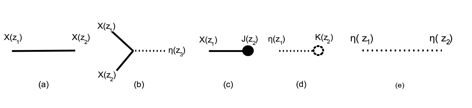
Figure 1: Feynmann diagrams associated with the field theory of eqn. (18). Also, each external line of η⁡(z)\eta(z) contributes with mm, while each external line of χ⁡(z)\chi(z) contributes 2​π​i2\pi i.

We now discuss the field theory properties of the model above. In Fig. 1 we show the Feynman diagrams associated with eqn. (18). For each point zz, one associates an integral ∮𝒞dzz−1⋅\oint_{\mathcal{C}}dz\ z^{-1}\cdot. Then, we have the following associated rules:

(a) =\displaystyle= 4​π2​J~−1​(z1,z2)\displaystyle 4\pi^{2}\tilde{J}^{-1}(z_{1},z_{2})
(b) =\displaystyle= −i4​π2​β​δ​(z3−z1−1​z2−1)\displaystyle-\frac{i}{4\pi^{2}\beta}\delta(z_{3}-z_{1}^{-1}z_{2}^{-1})
(c) =\displaystyle= −i​β2​π​h​(z2−1)\displaystyle-i\frac{\sqrt{\beta}}{2\pi}h(z_{2}^{-1})
(d) =\displaystyle= −δ⁡(z2−1)\displaystyle-\delta(z_{2}-1)
(e) =\displaystyle= −4​π2​m−2​δ​(z1−z2−1)\displaystyle-4\pi^{2}m^{-2}\delta(z_{1}-z_{2}^{-1}) (44)

In order to see whether this is correct, we can integrate out the field χ\chi explicitly, and write the effective action as

Z⁡(h⁡(z))\displaystyle Z(h(z)) =\displaystyle= ∫[dη]e−∮𝒞dzz−1(η(z)δ(z−1)−m24​π2η(z)η(z−1))+β22∮dz1dz2h(z1−1)h(z2−1)(η(z1−1z2−1)\displaystyle\int[d\eta]e^{-\oint_{\mathcal{C}}dzz^{-1}\left(\eta(z)\delta(z-1)-\frac{m^{2}}{4\pi^{2}}\eta(z)\eta(z^{-1})\right)+\frac{\beta^{2}}{2}\oint dz_{1}dz_{2}h(z_{1}^{-1})h(z_{2}^{-1})(\eta(z_{1}^{-1}z_{2}^{-1})}
⋅eOPENβ​J~​(z1,z2))−1​z1−1​z2−1−i2​Tr​log⁡(η⁡(z1−1​z2−1)+β​J~​(z1,z2))\displaystyle\ \ \ \ \ \cdot e^{\beta\tilde{J}(z_{1},z_{2}))^{-1}z_{1}^{-1}z_{2}^{-1}-\frac{i}{2}\text{Tr}\log(\eta(z_{1}^{-1}z_{2}^{-1})+\beta\tilde{J}(z_{1},z_{2}))}

which can be the beginning of a Loop-Vertex-Expansion as we realize that the action was in an intermediate field representation rivasseau. This possibility will considered in future works inprep.

4.3 A few examples

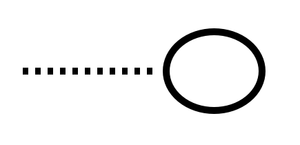
Let us now look at the effective interaction at the first order in TT for the field η\eta. As a first comment, we note that an effective external field is provided in Fig. 2 (top), which takes the form

Jη,e​f​f1​(z1)\displaystyle J^{1}_{\eta,eff}(z_{1}) =\displaystyle= −i​z1​T2​π∮𝒞dzz−1J~(z1z,z1−1z−1)\displaystyle-\frac{i\sqrt{z_{1}}T}{2\pi}\oint_{\mathcal{C}}dzz^{-1}\tilde{J}(\sqrt{z_{1}}z,\sqrt{z_{1}}^{-1}z^{-1}) (45)
=\displaystyle= z1​Trace​(J−1).\displaystyle\sqrt{z_{1}}\ \text{Trace}(J^{-1}).

We thus obtain that

Jη,e​f​f=δC​(z−1)+z​T​Z​QJ_{\eta,eff}=\delta_{C}(z-1)+\sqrt{z}T\sqrt{Z}Q (46)

with Q=Trace​(J−1)Q=\text{Trace}(J^{-1}), and depends on the traces of the Green function. This is a feature of diagrams with only external η\eta legs, and we see that it comes naturally in this formalism.

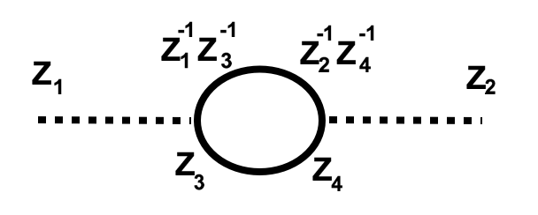
It is interesting to note that we can also introduce the effective propagator for the η\eta field, mediated via the χ\chi interaction. This is shown in Fig. 2 (right) and is given by

G⁡(z1,z2)\displaystyle G(z_{1},z_{2}) =\displaystyle= −(4​π2)2​z1​z2β2​Trace​(J−2)\displaystyle-\frac{(4\pi^{2})^{2}\sqrt{z_{1}z_{2}}}{\beta^{2}}\text{Trace}(J^{-2}) (47)

and we note that the term V=∑i​j(Ji​j−2)=Trace​(J−2)V=\sum_{ij}(J_{ij}^{-2})=\text{Trace}(J^{-2}), which is the sum of all the elements of the matrix Ji​jJ_{ij} squared is, in principle, divergent if not properly regularized.
Refer to caption
Refer to caption
Figure 2: External field and effective propagator for the η\eta field.

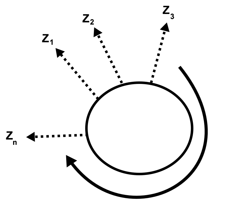
Since in what follows these diagrams are important, let us now consider the n−n-point function as in Fig. 3. We call these urchin diagrams and will be relevant later when we perform a double scaling limit.
Refer to caption
Refer to caption
Figure 3: The interaction vertex nn-point function for η​(z)n\eta(z)^{n} and its parametrization. We call these urchin diagrams.

The diagram can be written as:

Vn​(z1,⋯,zn)=Dn​(4​π2)2​nβn​(−i)n(4​π2)n​∮𝒞(∏i=1nd​z~i1​d​z~i2​(zi1)−1​(zi2)−1​J~−1​(z~i1,z~i2))​δ​(z1−z~n2​z~11)​∏k=1n−1δ⁡(zk−z~k2​z~k+11)V_{n}(z_{1},\cdots,z_{n})=D_{n}\frac{(4\pi^{2})^{2n}}{\beta^{n}}\frac{(-i)^{n}}{(4\pi^{2})^{n}}\oint_{\mathcal{C}}\left(\prod_{i=1}^{n}d\tilde{z}^{1}_{i}d\tilde{z}^{2}_{i}(z_{i}^{1})^{-1}(z_{i}^{2})^{-1}\tilde{J}^{-1}(\tilde{z}^{1}_{i},\tilde{z}^{2}_{i})\right)\delta(z_{1}-\tilde{z}_{n}^{2}\tilde{z}_{1}^{1})\prod_{k=1}^{n-1}\delta(z_{k}-\tilde{z}_{k}^{2}\tilde{z}_{k+1}^{1}) (48)

where DnD_{n} is a symmetry factor on which we will focus on later. We can rewrite the integral as

Vn​(z1,⋯,zn)\displaystyle V_{n}(z_{1},\cdots,z_{n}) =\displaystyle= Dn​(−i)n​(4​π2)nβn\displaystyle D_{n}(-i)^{n}\frac{(4\pi^{2})^{n}}{\beta^{n}}
⋅\displaystyle\cdot ∏i=1nzi​∮𝒞d​z~i​J~−1​(zn​z~n,z1−1​z~1−1)\displaystyle\prod_{i=1}^{n}\sqrt{z_{i}}\oint_{\mathcal{C}}d\tilde{z}_{i}\tilde{J}^{-1}(\sqrt{z_{n}}\tilde{z}_{n},\sqrt{z_{1}}^{-1}\tilde{z}_{1}^{-1})
⋅\displaystyle\cdot ∏i=1n−1J~−1​(zi​z~i,zi+1−1​z~i−1)\displaystyle\prod_{i=1}^{n-1}\tilde{J}^{-1}(\sqrt{z_{i}}\tilde{z}_{i},\sqrt{z_{i+1}}^{-1}\tilde{z}_{i}^{-1})
=\displaystyle= Dn​(−i)n​(4​π2)nβn​∏i=1nzi​(2​π​i)n​Trace​(J−n)\displaystyle D_{n}(-i)^{n}\frac{(4\pi^{2})^{n}}{\beta^{n}}\prod_{i=1}^{n}\sqrt{z_{i}}(2\pi i)^{n}\text{Trace}(J^{-n})
=\displaystyle= Dn​(2​π)3​n​Trace​(J−n)βn​∏i=1nzi\displaystyle D_{n}\frac{(2\pi)^{3n}\text{Trace}(J^{-n})}{\beta^{n}}\prod_{i=1}^{n}\sqrt{z_{i}}

We thus see that these diagrams are naturally associated with traces of powers of the Green function. We also now understand the role of the external field δC\delta_{C} for the η\eta auxiliary field in the combinatorics. For a symmetric tridiagonal matrix with zero elements on the diagonal and elements JJ of the upper and lower diagonals, the eigenvalues are given by 2​J​cos⁡(k​π(N+1))2J\cos(\frac{k\pi}{(N+1)}) for k=1⋯Nk=1\cdots N and NN is the number of spins.

5 Resummation of the low temperature expansion in a mass parameter rescaling

In this section we provide further background to the low temperature expansion, via constraining ourself to a very specific limit of the coupling constant, the temperature. Low temperature expansions for arbitrary couplings must necessarily be ill-defined. This is due to the Dyson argument for which, if the series expansion at T=0T=0 was convergent, then we the series would also be defined for T<0T<0, which from the point of view of Statistical Physics does not make sense. There are several known ways to avoid this situation: the first and most well known is to resort to renormalization, whether constructive, perturbative or non-perturbative. The second and simpler is to consider a subset of diagrams via coupling rescaling, and thus focus only on a certain phase of the model. We discuss the latter first.

5.1 Temperature rescaling

Refer to caption
Figure 4: Two diagrams contributing at order TT. Diagram (a)(a) is of order T2m\frac{T^{2}}{m}, while diagram (b)(b) is of order T2m2\frac{T^{2}}{m^{2}}.

Let us first discuss one possible well-defined way to perform the limit m→0m\rightarrow 0 diagrammatically. Each line of η\eta (both internal and external) contributes a factor of mm. For instance, in Fig. 4 we observe two diagrams which contribute at the order T2T^{2}. In the first, before rescaling, diagram (a)(a) gives T2m2\frac{T^{2}}{m^{2}}, meanwhile diagram (b)(b) is T2m4\frac{T^{2}}{m^{4}}. This is a general feature of the model: since for each interaction vertex there is a factor of TT associated, we can rescale T→T​m2T\rightarrow Tm^{2}, and the limit m→0m\rightarrow 0 implies that, at the order TkT^{k}, only diagrams with kk external η\eta lines dominate. The limit m→0m\rightarrow 0 then corresponds to the weak coupling regime which we are interested in. After the rescaling aforementioned, we see that the diagram (a) in Fig. 4 goes to zero in the limit m→0m\rightarrow 0. This implies, again, that for each internal lines of η\eta, at the same order of TT, the diagram acquires a factor mm after the rescaling of the temperature. This allows us to study only what we call urchin diagrams, e.g. diagrams with only external η\eta lines, and is reminishent of a Hartree-Fock approximatino. Using the device of the limit m→0m\rightarrow 0, we can also make sense of a low temperature expansion. We thus obtain that the limit:

limT,m→0GT,m(z1,⋯,zn) : Tm2=constant\lim_{T,m\rightarrow 0}G^{T,m}(z_{1},\cdots,z_{n})\text{ : }\frac{T}{m^{2}}=\text{constant} (49)

is equivalent to the urchin diagrams expansion for the partition function that we study below. We thus keep the ratio Tm2=T~\frac{T}{m^{2}}=\tilde{T} fixed. The expansion above is similar in spirit to the melonic expansion in a certain class of group field theories and in constructive field theory, and is thus equivalent to keeping diagrams with the higher superficial degree of infrared divergences. Alternatively, we can also consider the strong coupling case, in which T​mTm is constant in the limit m→0m\rightarrow 0. In this case, the external field interactions are set to zero, while diagram (a) in Fig. 4 effectively becomes the contraction of an effective propagator for a non quadratic theory (as the propagator for η⁡(z)\eta(z) is 1m​δ​(z−z−1)\frac{1}{m}\delta(z-z^{-1})): in this limit we reobtain Landau-Ginzburg interactions, and η\eta becomes an intermediate field representation for ϕ4\phi^{4} theory. The strong coupling regime will be discussed elsewhere.

5.2 Combinatorics of closed loops, and set partitions

Since we have argued that the double scaling limit above is a summation with only urchi diagrams, it is worth spending some time to explain the combinatorics of these diagrams.

Given the urchin diagrams expansions above, we now discuss how to evaluate Feynman diagrams and the coefficient DnD_{n} in a bit more detail. The evaluation of the Feynman diagrams takes advantage of few properties of the complex integrations we have mentioned before. At the order TkT^{k}, we have kk vertices. Since the field η\eta does not propagate internally after the rescaling, the only possibility is that these appear as external fields. For the partition function at h=0h=0, this implies for ZZ that only diagrams with amputated legs of η\eta will appear. We define Gnc(z11,z12⋯,zn1,zn2)G_{n}^{c}(z_{1}^{1},z_{1}^{2}\cdots,z_{n}^{1},z_{n}^{2}) the connected diagrams with kk vertices and 2​n2n internal χ\chi legs. For each external η\eta leg, there is a factor of δ⁡(z−1)\delta(z-1). Since the external legs necessarily connect only to two internal legs, and if all internal legs are contracted, we have locally terms of the form

12​π​i∮𝒞\displaystyle\frac{1}{2\pi i}\oint_{\mathcal{C}} d⁡[z]\displaystyle d[z] d​zη​d​ze′1​ze′2​ze1​d​ze2​Q𝒢\{e,e′}​([z])\displaystyle dz_{\eta}dz_{e^{\prime}}^{1}z_{e^{\prime}}^{2}z_{e}^{1}dz_{e}^{2}Q_{\mathcal{G}\backslash\{e,e^{\prime}\}}([z]) (50)
⋅\displaystyle\cdot J−1​(ze1,ze2)​J−1​(ze′1,ze′2)\displaystyle J^{-1}(z_{e}^{1},z_{e}^{2})J^{-1}(z_{e^{\prime}}^{1},z_{e^{\prime}}^{2})
⋅\displaystyle\cdot δ⁡(zη−(ze2)−1​(ze′1)−1​δ​(zη−1)CLOSE\displaystyle\delta(z_{\eta}-(z_{e}^{2})^{-1}(z_{e^{\prime}}^{1})^{-1}\delta(z_{\eta}-1)

where d⁡[z]d[z] contain integration over the rest of the internal legs and ze1,ze′2z_{e}^{1},z_{e^{\prime}}^{2}, and Q𝒢\{e,e′}​([z])Q_{\mathcal{G}\backslash\{e,e^{\prime}\}}([z]) represents the rest of the graph. We see immediately that we can integrate out the external field δ⁡(zη−1)\delta(z_{\eta}-1) and the vertex, and impose ze2=(ze′1)−1z_{e}^{2}=(z_{e^{\prime}}^{1})^{-1}. This is the equivalent of the scalar product between the Green functions:

12​π​i​∮𝒞d​ze′1​J−1​(ze1,(ze′1)−1)​J−1​(ze′1,ze′2)=J−2​(ze1,ze′2).\frac{1}{2\pi i}\oint_{\mathcal{C}}dz_{e^{\prime}}^{1}J^{-1}(z_{e}^{1},(z_{e^{\prime}}^{1})^{-1})J^{-1}(z_{e^{\prime}}^{1},z_{e^{\prime}}^{2})=J^{-2}(z_{e}^{1},z_{e^{\prime}}^{2}).

This is all we need to evaluate amputated diagrams in the following.

For the case of the partition function, we thus need to consider all possible closed loops, as there are no external χ\chi amputated lines, while for the case of n−p​o​i​n​tn-point functions of χ\chi, there can be open lines. However, it is easy to see that for closed lines necessarily we must have, following the integrations:

12​π​i​∮𝒞d​ze1​J−k​(ze1,(ze1)−1)=Trace​(J−k​(ze1,ze′2)).\frac{1}{2\pi i}\oint_{\mathcal{C}}dz_{e}^{1}J^{-k}(z_{e}^{1},(z_{e}^{1})^{-1})=\text{Trace}\left(J^{-k}(z_{e}^{1},z_{e^{\prime}}^{2})\right). (51)

Thus, for an operator Q⁡(z1,z2)Q(z_{1},z_{2}), the trace is defined as

Trace​(Q)=12​π​i​∮𝒞d​z1​d​z2z1​z2​δ​(z1−z2−1)​Q​(z1,z2).\text{Trace}(Q)=\frac{1}{2\pi i}\oint_{\mathcal{C}}\frac{dz_{1}dz_{2}}{z_{1}z_{2}}\delta(z_{1}-z_{2}^{-1})Q(z_{1},z_{2}). (52)

The result above shows that for each closed loop in 𝒢\mathcal{G} we associate a trace over a power of the Green function which is the length of the loop. In principle this could help in evaluating the coefficients in the Feynman diagrams.

Let us now use this result in conjunction with an exact mapping between the Feynmann diagrams with the set partitions. First we note that the combinatorial factor associated with a loop of length rr is 2r−1​(r−1)!2^{r-1}(r-1)! due to the various ways in which 2-legs of a graph can be joint to make a loop. This factor is due to the mechanics of Wick contractions and the automorphism group of a cycle.

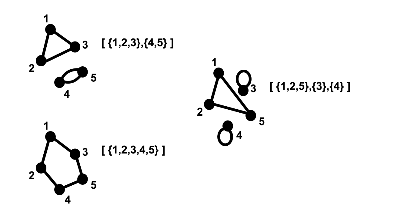
In order to see the connection with the set partitions, let us now label the nn-vertices of a graph as v1,⋯,vnv_{1},\cdots,v_{n}. It is easy to see that there is a one to one mapping to set partitions, as in Fig. 5, and more specifically the partition of integers. For each cycle among nodes, we write the loop as a order-indendent partition of the nodes. To each partition between nn nodes, corresponds a certain value of the Feynman diagram. For instance, to the sets [{1,2,3},{4,5}][\{1,2,3\},\{4,5\}], [{1,2,3,4,5}][\{1,2,3,4,5\}] and [{1,2,5},{3},{4}][\{1,2,5\},\{3\},\{4\}], correspond Trace​(J−3)​Trace​(J−2)\text{Trace}\left(J^{-3}\right)\text{Trace}\left(J^{-2}\right), Trace​(J−5)\text{Trace}\left(J^{-5}\right) and Trace​(J−3)​(Trace​(J−1))2\text{Trace}\left(J^{-3}\right)\left(\text{Trace}\left(J^{-1}\right)\right)^{2} respectively, and obviously independently of the labelling of the nodes. We need, thus, to count identical partitions among the nodes in order to obtain the coefficient in front of a certain value of a Feynman diagram. We can thus write the sum over graphs 𝒢\mathcal{G} as a sum over set partitions, where the coefficients are the associated partitions of integers. Let π∈Π⁡(k)\pi\in\Pi(k) be a certain partition of an integer kk, {n1,⋯,np}\{n_{1},\cdots,n_{p}\}, such that ∑ini=k\sum_{i}n_{i}=k, ni∈ℕn_{i}\in\mathbb{N} and PfP_{f} the number of such identical partition of the set (here nin_{i} can be degenerate). Each loop of length nin_{i} will give a factor Trace​(J−ni)\text{Trace}(J^{-n_{i}}), but if there are many loops of identical length gig_{i}, there will be a factor Trace​(J−ni)gi\text{Trace}(J^{-n_{i}})^{g_{i}} in that diagram.

In order to calculate the combinatorial coefficient, we write the partition of the integer as a sum over the nondegenerate blocks toufik:

∑i=1|π|gi​ni=k\sum_{i=1}^{|\pi|}g_{i}n_{i}=k

where gig_{i} is the number of partitions of identical size nin_{i}, and nin_{i} are all distinct. For instance for a Feynman graph with 3-nodes, we will have

π1→ 3\displaystyle\pi_{1}\rightarrow\ 3 =\displaystyle= 1+1+1=3⋅1\displaystyle 1+1+1=3\cdot 1
π2→ 3\displaystyle\pi_{2}\rightarrow\ 3 =\displaystyle= 2+1\displaystyle 2+1
π3→ 3\displaystyle\pi_{3}\rightarrow\ 3 =\displaystyle= 3\displaystyle 3 (53)

which implies |Π⁡(3)|=3|\Pi(3)|=3, and we have |π1|=3,|π2|=2,|π3|=1|\pi_{1}|=3,|\pi_{2}|=2,|\pi_{3}|=1. The degeneracy of the size is thus encoded in the factor gig_{i}. The formula above clearly classifies all partitions of integers. Then, we know that given gig_{i} and nin_{i}, the total number of such partitions has a formula which is k!gi!​(ni!)gi\frac{k!}{g_{i}!(n_{i}!)^{g_{i}}}. For π1\pi_{1}, we have only one block of degeneracy gi=3g_{i}=3, for π2\pi_{2} we have two blocks both of degeneracy gi=1g_{i}=1, and in π3\pi_{3} we have one block of degeneracy 1.

We thus have the formula

O(Tk):k!∑π∈Π⁡(k)∏Bi∈π|π|((ni−1)!​2(ni−1))gigi!​(ni!)gi(Tr(J−ni))gi.O(T^{k}):\ \ k!\sum_{\pi\in\Pi(k)}\prod_{B_{i}\in\pi}^{|\pi|}\frac{\left((n_{i}-1)!2^{(n_{i}-1)}\right)^{g_{i}}}{g_{i}!(n_{i}!)^{g_{i}}}(\text{Tr}\left(J^{-n_{i}}\right))^{g_{i}}. (54)

For k=2k=2, there are only 3 contractions, of which 2 gives identical terms. For k=3k=3 we have 15 contractions, meanwhile for k=4k=4 we have 105 contractions. We will use the formula above in the following in order to check whether the coefficients are correct. For k=1k=1, the only diagram is the tadpole which gives at the order O⁡(T)O(T), Trace​(J−1)\text{Trace}(J^{-1}). The combinatorial coefficients become already non-trivial at the subsequent order, where we have two partitions of the integer 2, 2=1+12=1+1 (gi=2g_{i}=2, ni=1n_{i}=1) and 2=22=2 (gi=1g_{i}=1, ni=2n_{i}=2):

O⁡(T~2)\displaystyle O(\tilde{T}^{2}) :\displaystyle: 12!​(21​(2−1)​2!1!​(2!)1​Tr​(J−2)+22​(1−1)​2!2!​(1!)2​(Tr​(J−1))2)\displaystyle\ \ \frac{1}{2!}\Big(\frac{2^{1(2-1)}2!}{1!(2!)^{1}}\ \text{Tr}(J^{-2})+\frac{2^{2(1-1)}2!}{2!(1!)^{2}}\left(\text{Tr}(J^{-1})\right)^{2}\Big)
=\displaystyle= 12!​(2​Tr​(J−2)+(Tr​(J−1))2)\displaystyle\ \ \frac{1}{2!}\Big(2\ \text{Tr}(J^{-2})+\left(\text{Tr}(J^{-1})\right)^{2}\Big)

For instance, let us consider k=3k=3, 3=2+1=1+1+13=2+1=1+1+1. There is one partition with one block g1=3g_{1}=3 n1=1n_{1}=1, one partition with two blocks g1=1g_{1}=1, n1=2n_{1}=2, and g2=1g_{2}=1 n2=2n_{2}=2 and one partition with one block g1=1g_{1}=1 and n1=3n_{1}=3. Thus, we immediately obtain

O(T~3):13!(8Tr(J−3)\displaystyle O(\tilde{T}^{3}):\ \ \frac{1}{3!}\Big(8\ \text{Tr}(J^{-3}) +\displaystyle+ 6​Tr​(J−2)​Tr​(J−1)\displaystyle 6\ \text{Tr}(J^{-2})\text{Tr}(J^{-1}) (56)
+\displaystyle+ OPEN(Tr​(J−1))3).\displaystyle\left(\text{Tr}(J^{-1})\right)^{3}\Big).
Refer to caption
Figure 5: Example of the mapping between graphs and the indices of integer partitions. Effectively, the combinatorics is the one of a loop gas.

At the order O⁡(T~4)O(\tilde{T}^{4}), we have 105 Isserlis-Wick possible contractions. We have five possible partitions, 4=1+1+1+1=2+2=3+1=2+1+14=1+1+1+1=2+2=3+1=2+1+1. We thus obtain from our formula,

O(T~4):14!(\displaystyle O(\tilde{T}^{4}):\ \ \frac{1}{4!}\Big( 48\displaystyle 48 Tr​(J−4)+32​Tr​(J−3)​Tr​(J−1)\displaystyle\ \text{Tr}(J^{-4})+32\ \text{Tr}(J^{-3})\text{Tr}(J^{-1}) (57)
+\displaystyle+ 12​(Tr​(J−2))2+(Tr​(J−1))4\displaystyle 12\left(\text{Tr}(J^{-2})\right)^{2}+\left(\text{Tr}(J^{-1})\right)^{4}
+\displaystyle+ OPEN12​(Tr​(J−1))2​Tr​(J−2))\displaystyle 12\left(\text{Tr}(J^{-1})\right)^{2}\text{Tr}(J^{-2})\Big)

and the coefficients sum up to 105105 as one would expect.

5.3 Resummation

From the previous sections, we see that in the double-scaling limit we can thus write the partition function as

Z=∑k=0∞Tk​∑π∈Π⁡(k)∏Bi∈π|π|1gi!​(2ni−1​Tr​(J−ni)ni)gi.Z=\sum_{k=0}^{\infty}T^{k}\sum_{\pi\in\Pi(k)}\prod_{B_{i}\in\pi}^{|\pi|}\frac{1}{g_{i}!}\left(\frac{2^{n_{i}-1}\text{Tr}\left(J^{-n_{i}}\right)}{n_{i}}\right)^{g_{i}}. (58)

The formula above is thus connected to the spectral properties of the coupling matrix JJ. Let us now try to write this sum in a less combinatorial way. First, we note that we can write Tk=T∑ii​giT^{k}=T^{\sum_{i}ig_{i}}. For each number kk, we can write ∑Π⁡(k)\sum_{\Pi(k)} as follows :

∑π∈Π⁡(k)→∮d​z2​π​i∑g1,⋯,gk=0∞1zk+1−∑i=1ki​gi.\sum_{\pi\in\Pi(k)}\rightarrow\oint\frac{dz}{2\pi i}\sum_{g_{1},\cdots,g_{k}=0}^{\infty}\frac{1}{z^{k+1-\sum_{i=1}^{k}ig_{i}}}. (59)

Something that will however provide an analytical final formula is the following remark. It is interesting to note that we can write also

∑i=1k~i​gi=k,\sum_{i=1}^{\tilde{k}}ig_{i}=k, (60)

with gi∈ℕg_{i}\in\mathbb{N} and k~≥k\tilde{k}\geq k. We know however that for i>ki>k, gi=0g_{i}=0. As a quick check of this fact, note the following. Consider k=3k=3 and ∑i=13i​gi=k\sum_{i=1}^{3}ig_{i}=k, for which we have only 3=1+1+1=1+23=1+1+1=1+2. From the integral formula we have introduced, we obtain Res​(1z4​∏j=1k~(1−zj),0)=3\text{Res}(\frac{1}{z^{4}\prod_{j=1}^{\tilde{k}}(1-z^{j})},0)=3, ∀k~≥3\forall\tilde{k}\geq 3, which is true as it can be promptly checked. This implies that we can write term by term an infinite sum over zeros in the expansion, as we will see in a moment.

We can write the constrained sum using an integral over the complex plane, via the imposition of the constraint of eqn. (60) using eqn. (59). We have then,

∑π∈Π⁡(k)∏Bi∈π|π|1gi!​(2ni−1​Tr​((TJ)−ni)ni)gi\displaystyle\sum_{\pi\in\Pi(k)}\prod_{B_{i}\in\pi}^{|\pi|}\frac{1}{g_{i}!}\left(\frac{2^{n_{i}-1}\text{Tr}\left((\frac{T}{J})^{-n_{i}}\right)}{n_{i}}\right)^{g_{i}} =\displaystyle= ∮d​z2​π​i​∑g1,⋯,gk~=0∞1zk+1−∑i=1k~i​gi​∏i=1k~1gi!​(2i−1​Tr​((TJ)−i)i)gi\displaystyle\oint\frac{dz}{2\pi i}\sum_{g_{1},\cdots,g_{\tilde{k}}=0}^{\infty}\frac{1}{z^{k+1-\sum_{i=1}^{\tilde{k}}ig_{i}}}\prod_{i=1}^{\tilde{k}}\frac{1}{g_{i}!}\left(\frac{2^{i-1}\text{Tr}\left((\frac{T}{J})^{-i}\right)}{i}\right)^{g_{i}} (61)
=\displaystyle= ∮d​z2​π​i​1zk+1​∏i=1k~∑gi=0∞1gi!​(2i−1​zi​Tr​((TJ)−i)i)gi\displaystyle\oint\frac{dz}{2\pi i}\frac{1}{z^{k+1}}\prod_{i=1}^{\tilde{k}}\sum_{g_{i}=0}^{\infty}\frac{1}{g_{i}!}\left(\frac{2^{i-1}z^{i}\text{Tr}\left((\frac{T}{J})^{-i}\right)}{i}\right)^{g_{i}}
=\displaystyle= ∮d​z2​π​i​1zk+1​e12​∑i=1k~2i​zi​Tr​((TJ)−i)i\displaystyle\oint\frac{dz}{2\pi i}\frac{1}{z^{k+1}}e^{\frac{1}{2}\sum_{i=1}^{\tilde{k}}\frac{2^{i}z^{i}\text{Tr}\left((\frac{T}{J})^{-i}\right)}{i}}
=\displaystyle= ∮d​z2​π​i​1zk+1​e12​∑n=1N∑i=1k~2i​Ti​ziλni​i,\displaystyle\oint\frac{dz}{2\pi i}\frac{1}{z^{k+1}}e^{\frac{1}{2}\sum_{n=1}^{N}\sum_{i=1}^{\tilde{k}}\frac{2^{i}T^{i}z^{i}}{\lambda_{n}^{i}i}},

where we have identified ni=in_{i}=i. We now use the identity

∑i=1k~xii=xk~+1​(−Φ⁡(x,1,k~+1))−log⁡(1−x),\sum_{i=1}^{\tilde{k}}\frac{x^{i}}{i}=x^{\tilde{k}+1}(-\Phi(x,1,\tilde{k}+1))-\log(1-x), (62)

where Φ⁡(x,1,k+1)\Phi(x,1,k+1) is the Lerch Zeta-function, defined as

Φ⁡(x,s,z)=∑j=0∞xj(j+z)s.\Phi(x,s,z)=\sum_{j=0}^{\infty}\frac{x^{j}}{(j+z)^{s}}. (63)

We now reconsider the normalization that we had ignored insofar. We then obtain the following representation for the partition function for finite k~\tilde{k}:

𝒵k~​(T)\displaystyle\mathcal{Z}_{\tilde{k}}(T) =\displaystyle= ZGauss(T)∮d​z2​π​iFk~(z,λ)e−12∑n=1Nlog(1−2​z​Tλn)\displaystyle Z_{\text{Gauss}}(T)\oint\frac{dz}{2\pi i}F_{\tilde{k}}(z,\lambda)e^{-\frac{1}{2}\sum_{n=1}^{N}\log(1-\frac{2zT}{\lambda_{n}})} (64)
=\displaystyle= ZGauss​(T)​∮d​z2​π​i​Fk~​(z,λ)∏i=1N1−2​z​Tλi\displaystyle Z_{\text{Gauss}}(T)\oint\frac{dz}{2\pi i}\frac{F_{\tilde{k}}(z,\lambda)}{\prod_{i=1}^{N}\sqrt{1-\frac{2zT}{\lambda_{i}}}}

with

Fk~(z,λ)=∑k=0k~1zk+1e−12∑n=1N(2​zλn)k~+1Φ(2​zλn,1,k~+1).F_{\tilde{k}}(z,\lambda)=\sum_{k=0}^{\tilde{k}}\frac{1}{z^{k+1}}e^{-\frac{1}{2}\sum_{n=1}^{N}(\frac{2z}{\lambda_{n}})^{\tilde{k}+1}\Phi(\frac{2z}{\lambda_{n}},1,\tilde{k}+1)}.

We would like to obtain a better expression from the above, and what we get can be intended in two ways. First, we are interested in the asymptotic values of the sum in FF, from which we can simply take

F⁡(z,λ)≈1z​∑k=0∞1zk≈1z−1.F(z,\lambda)\approx\frac{1}{z}\sum_{k=0}^{\infty}\frac{1}{z^{k}}\approx\frac{1}{z-1}. (65)

Alternatively, we can consider the limit

limk~→∞Zk~⟹limk~→∞∑j=0k~xjj=−log⁡(1−x),\lim_{\tilde{k}\rightarrow\infty}Z_{\tilde{k}}\implies\lim_{\tilde{k}\rightarrow\infty}\sum_{j=0}^{\tilde{k}}\frac{x^{j}}{j}=-\log(1-x), (66)

that as we as seen should not contribute to the integral. In both cases, we obtain the expression

𝒵⁡(T)=ZGauss​(T)​∮d​z2​π​i​e−12∑n=1Nlog(1−2​z​Tλn)(z−1).\mathcal{Z}(T)=Z_{\text{Gauss}}(T)\oint\frac{dz}{2\pi i}\frac{e^{-\frac{1}{2}\sum_{n=1}^{N}\log(1-\frac{2zT}{\lambda_{n}})}}{(z-1)}. (67)

We can rewrite this equation more succintly in terms of the spectral density for the matrix JJ, as

𝒵⁡(T)=ZGauss​(T)​∮d​z2​π​i​e−12∮dλρJ(λ)log(1−2​z​Tλ)(z−1),\mathcal{Z}(T)=Z_{\text{Gauss}}(T)\oint\frac{dz}{2\pi i}\frac{e^{-\frac{1}{2}\oint d\lambda\rho_{J}(\lambda)\log(1-\frac{2zT}{\lambda})}}{(z-1)}, (68)

which is our final expression, with

ρJ​(λ)=∑λi∈Λ⁡(J)δ⁡(λ−λi).\rho_{J}(\lambda)=\sum_{\lambda_{i}\in\Lambda(J)}\delta(\lambda-\lambda_{i}). (69)

We have thus rewritten the partition function of the Ising model in terms of its spectral representation only. It is worth mentioning that this representation is rather hard to interpret, as it involved branch cuts in the complex plane that are due to the position of the eigenvalues of JJ. However, we note that there is the emergence of a non-perturbative pole at z=1z=1, and it would be tempting to enlarge the domain to enclose it. It is not clear whether this procedure is however correct.

Another way of treating the partition function is via the tricks used in the study of the f-Mayer expansion, or linked cluster expansion Huang. We start from

Z=∑k=0∞Tk​∑π∈Π⁡(k)∏Bi∈π|π|1gi!​(2ni−1​Tr​(J−ni)ni)gi.Z=\sum_{k=0}^{\infty}T^{k}\sum_{\pi\in\Pi(k)}\prod_{B_{i}\in\pi}^{|\pi|}\frac{1}{g_{i}!}\left(\frac{2^{n_{i}-1}\text{Tr}\left(J^{-n_{i}}\right)}{n_{i}}\right)^{g_{i}}. (70)

and note that we can write it as

Z\displaystyle Z =\displaystyle= ∑g1=0∞⋯∑gN=0∞∏i1gi!(2i−1​Tr​(J−i)iTi)gi,\displaystyle\sum_{g_{1}=0}^{\infty}\cdots\sum_{g_{N}=0}^{\infty}\prod_{i}\frac{1}{g_{i}!}\left(\frac{2^{i-1}\text{Tr}\left(J^{-i}\right)}{i}T^{i}\right)^{g_{i}}, (71)
=\displaystyle= e∑i=1∞2i−1​Tr​(J−i)i​Ti\displaystyle e^{\sum_{i=1}^{\infty}\frac{2^{i-1}\text{Tr}\left(J^{-i}\right)}{i}T^{i}}
=\displaystyle= e−12∫dλρ(λ)log(1−2​Tλ).\displaystyle e^{-\frac{1}{2}\int d\lambda\rho(\lambda)\log(1-\frac{2T}{\lambda})}.

It is interesting to note that the expression above is exactly the one we would have obtained from eqn. (68) by calculating the residue in z=1z=1 rather than z=0z=0. In this sense, the non-perturbative residue is not near the perturbative one.

Now we can obtain that

F\displaystyle F =\displaystyle= −κ​T​log⁡𝒵\displaystyle-\kappa T\log\mathcal{Z}
=\displaystyle= −κ​T​log⁡ZGauss​(T)+κ​T2​∫d​λ​ρ​(λ)​log⁡(1−2​Tλ)\displaystyle-\kappa T\log Z_{\text{Gauss}}(T)+\frac{\kappa T}{2}\int d\lambda\rho(\lambda)\log(1-\frac{2T}{\lambda})

where

−κ​T​log⁡ZGauss​(T)=κ​T2​log​detβ​J=κ​T2​∫d​λ​ρ​(λ)​log​β​λ2-\kappa T\log Z_{\text{Gauss}}(T)=\frac{\kappa T}{2}\log\det\beta J=\frac{\kappa T}{2}\int d\lambda\rho(\lambda)\log\frac{\beta\lambda}{2} (72)

from which we get

F=−κ​T​log⁡𝒵=κ​T2​∫d​λ​ρ​(λ)​log⁡(β​λ2−1)F=-\kappa T\log\mathcal{Z}=\frac{\kappa T}{2}\int d\lambda\rho(\lambda)\log\left(\frac{\beta\lambda}{2}-1\right) (73)

Let us now look at the case of a DD-dimensional lattice of size LL. The eigenvalues, in this case, are known to be parametrized as

λ⁡(n1,⋯,nD)=2​a+2​b​∑i=1Dcos⁡(2​πL​ni)\lambda(n_{1},\cdots,n_{D})=2a+2b\sum_{i=1}^{D}\cos(\frac{2\pi}{L}n_{i}) (74)

for n1=0,⋯,L−1n_{1}=0,\cdots,L-1. We can thus write the integral above as (we take the continuous limit):

F\displaystyle F =\displaystyle= −κ​T​log⁡𝒵\displaystyle-\kappa T\log\mathcal{Z}
=\displaystyle= κ​T​LD2​(2​π)D​∫02​πd​pD​log⁡(β⁡(a+b​∑i=1Dcos⁡p)−1)\displaystyle\frac{\kappa TL^{D}}{2(2\pi)^{D}}\int_{0}^{2\pi}dp^{D}\log\left(\beta(a+b\sum_{i=1}^{D}\cos p)-1\right)

The free energy per spin and per unit of energy can be written as

fκ​T\displaystyle\frac{f}{\kappa T} =\displaystyle= FLD​κ​T\displaystyle\frac{F}{L^{D}\kappa T}
=\displaystyle= 1(2​π)D​∫02​πd​pD​log⁡(β⁡(a+b​∑i=1Dcos⁡p)−1)\displaystyle\frac{1}{(2\pi)^{D}}\int_{0}^{2\pi}dp^{D}\log\left(\beta(a+b\sum_{i=1}^{D}\cos p)-1\right)

and look at its internal energy per site (at zero magnetic field), given by

u(T)=−T2∂Tfκ​Tu(T)=-T^{2}\partial_{T}\frac{f}{\kappa T} (75)

and the specific heat,

c⁡(T)=∂Tu⁡(T).c(T)=\partial_{T}u(T). (76)

We obtain the expression for the internal energy (we set κ=1\kappa=1):

u⁡(T)=1(2​π)D​∫02​πd​pD​T⁡(a+b​∑i=1Dcos⁡p)((a+b​∑i=1Dcos⁡p)−T)u(T)=\frac{1}{(2\pi)^{D}}\int_{0}^{2\pi}dp^{D}\frac{T(a+b\sum_{i=1}^{D}\cos p)}{\left((a+b\sum_{i=1}^{D}\cos p)-T\right)} (77)

We now use the standard trick of writing the inverse as

1λ=∫0∞d​t​e−t​λ\frac{1}{\lambda}=\int_{0}^{\infty}dte^{-t\lambda} (78)

and obtain (we assume that we are in an analytical region):

u⁡(T)=∫0∞d​t​T(2​π)D​∫02​πd​pD​(a+b​∑i=1Dcos⁡p)​e−t⁡((a+b​∑i=1Dcos⁡p)−T)u(T)=\int_{0}^{\infty}dt\frac{T}{(2\pi)^{D}}\int_{0}^{2\pi}dp^{D}(a+b\sum_{i=1}^{D}\cos p)e^{-t\left((a+b\sum_{i=1}^{D}\cos p)-T\right)} (79)

This term can be written in two parts:

u⁡(T)\displaystyle u(T) =\displaystyle= a​T​∫0∞d​t​e−t⁡(a−T)​J0​(−i​b​t)D\displaystyle aT\int_{0}^{\infty}dt\ e^{-t(a-T)}J_{0}(-ibt)^{D} (80)
+\displaystyle+ b​D​T​∫0∞d​t​e−t⁡(a−T)​J1​(−i​b​t)D.\displaystyle bDT\int_{0}^{\infty}dt\ e^{-t(a-T)}J_{1}(-ibt)^{D}.

Asymptotically (t≫1t\gg 1), we see that

Jα​(−i​b​t)≈12​π​b​t​(cos⁡(−i​b​t−π4)​(2​α+1))J_{\alpha}(-ibt)\approx\frac{1}{\sqrt{2\pi bt}}(\cos(-ibt-\frac{\pi}{4})(2\alpha+1)) (81)

Thus for b<0b<0 and t≫1t\gg 1 we obtain

u⁡(T)\displaystyle u(T) =\displaystyle= 2​(a+b​D)​T​∫0∞d​t​e−t⁡(a+b​D−T)(2​π​b​t)D2.\displaystyle 2(a+bD)T\int_{0}^{\infty}dt\ \frac{e^{-t(a+bD-T)}}{(2\pi bt)^{\frac{D}{2}}}. (82)

which the internal energy as a function of TT. Thus, the resummation of Urchin diagrams is not completely trivial, e.g. we do not reobtain the Gaussian theory.

6 Interactions with the external field

Before we go into the final remarks, we would like to discuss the interactions when also the external field hh is included. Let us consider the full model using the Green connected functions, defined as

Gn,connn,k​(z1,⋯,zn,z~1,⋯,z~k)G_{n,\text{conn}}^{n,k}(z_{1},\cdots,z_{n},\tilde{z}_{1},\cdots,\tilde{z}_{k}) (83)

is all the connected diagrams which satisfy the Feynman rules. We now note that since the only interacting vertex has two χ\chi lines and one η\eta lines, and the η\eta field does not propagate, the number interacting vertices equals to the number of outgoing η\eta lines. We have that the generator of connected diagrams

W⁡(hη,hχ)\displaystyle W\left(h_{\eta},h_{\chi}\right) ≡\displaystyle\equiv log⁡(Z⁡(Jη,Jχ))\displaystyle\log\left(Z\left(J_{\eta},J_{\chi}\right)\right) (84)
=\displaystyle= ∑n=0∞1n!​∑k=0n2∮𝒞Gn,c​o​n​nn,2​k​(z1,⋯,zn,z~1,⋯,z~2​k)\displaystyle\sum_{n=0}^{\infty}\frac{1}{n!}\sum_{k=0}^{\frac{n}{2}}\oint_{\mathcal{C}}G^{n,2k}_{n,conn}(z_{1},\cdots,z_{n},\tilde{z}_{1},\cdots,\tilde{z}_{2k})
⋅\displaystyle\cdot ∏i=1nhη​(zi)​zi−1​d​zi​∏r=1kβ​hχ​(z~r)​z~r−1​d​z~r\displaystyle\prod_{i=1}^{n}h_{\eta}(z_{i})z_{i}^{-1}dz_{i}\prod_{r=1}^{k}\beta h_{\chi}(\tilde{z}_{r})\tilde{z}_{r}^{-1}d\tilde{z}_{r}

where we have introduced hη​(z)=i​δ​(z−1)h_{\eta}(z)=i\delta(z-1), while hχ​(z)=h⁡(z−1)h_{\chi}(z)=h(z^{-1}). We now note that for each propagator, we contribute a factor of β−1\beta^{-1}. A rapid calculation will show that for each hχh_{\chi} there is a factor of β\beta and for each vertex there are two lines χ\chi. If k=0k=0, since only χ\chi fields can be contracted, we have a factor of β−n\beta^{-n}. For each external χ\chi field, we have two external factors β\beta and one due to losing one internal propagators. This implies that, since kk must be even, we have that

We see then that in order to write an expansion in powers of β−q\beta^{-q}, we can order them according to:

−n+32​k=−q→(n,2​k)=(3​p+q,2​k)-n+\frac{3}{2}k=-q\rightarrow(n,2k)=\left(3p+q,2k\right) (85)

with 2​p≤n2p\leq n, from which we can derive the table for the pair (n,2​k)(n,2k) at each perturbation order in β−1=T\beta^{-1}=T.

β−q\beta^{-q} k=0k=0 k=1k=1 k=2k=2 k=3k=3 ⋯\cdots
β−1\beta^{-1} (1,0)(1,0) (4,1)(4,1) (7,4)(7,4) (11,6)(11,6) ⋯\cdots
β−2\beta^{-2} (2,0)(2,0) (5,2)(5,2) (8,4)(8,4) (12,6)(12,6) ⋯\cdots
β−3\beta^{-3} (3,0)(3,0) (6,2)(6,2) (9,4)(9,4) (13,6)(13,6) ⋯\cdots
β−4\beta^{-4} (4,0)(4,0) (7,2)(7,2) (10,4)(10,4) (14,6)(14,6) ⋯\cdots
⋮\vdots ⋮\vdots ⋮\vdots ⋮\vdots ⋮\vdots ⋮\vdots
Table 1: Diagrams contributing to the same order in β−1\beta^{-1}. We see that for each order, an infinity of diagrams contribute if h≠0h\neq 0.

In Tab. 1 we show that if an external field hχh_{\chi} is present, an infinite tower of diagrams contribute to the same order in perturbation theory. This implies that this perturbation theory is well defined only for h=0h=0, in which the number of interaction vertices equals the number of external legs. Thus, in order for the perturbation to make sense, either one sets hχ=0h_{\chi}=0 or performs a background field expansion. Let us thus consider first hχ=0h_{\chi}=0.

W⁡[hη]=∑n=0∞(4​π2)nβn​n!​∮𝒞d​z1\displaystyle W[h_{\eta}]=\sum_{n=0}^{\infty}\frac{(4\pi^{2})^{n}}{\beta^{n}n!}\oint_{\mathcal{C}}dz_{1} ⋯\displaystyle\cdots d​zn​Gc​o​n​nn​(z1,⋯,zn)\displaystyle dz_{n}G^{n}_{conn}(z_{1},\cdots,z_{n}) (86)
⋅\displaystyle\cdot hη(z1)⋯hη(zn)\displaystyle h_{\eta}(z_{1})\cdots h_{\eta}(z_{n})

It is easy to see that 𝔼⁡[χ⁡(z)]=0\mathbb{E}[\chi(z)]=0 if hχ=0h_{\chi}=0. If also J=0J=0, which is equivalent to the tree level, then the only diagram which is viable is the vertex, and also the only diagram which contributes at the zeroth order. We have

𝔼⁡[χ⁡(z1)​χ​(z2)]\displaystyle\mathbb{E}[\chi(z_{1})\chi(z_{2})] =\displaystyle= (2​π​i)2​i4​π2​∮d​z​z−1​δ​(z−z1−1​z2−1)​δ​(z−1)\displaystyle(2\pi i)^{2}\frac{i}{4\pi^{2}}\oint dz\ z^{-1}\delta(z-z_{1}^{-1}z_{2}^{-1})\delta(z-1) (87)
=\displaystyle= δ⁡(1−z1−1​z2−1)\displaystyle\delta(1-z_{1}^{-1}z_{2}^{-1})

Thus

𝔼[σiσj]=−14​π2∮dz1z1idz2z2j𝔼[χ(z1)χ(z2)]=δi​j\mathbb{E}[\sigma_{i}\sigma_{j}]=-\frac{1}{4\pi^{2}}\oint dz_{1}z_{1}^{i}dz_{2}z_{2}^{j}\mathbb{E}[\chi(z_{1})\chi(z_{2})]=\delta_{ij} (88)

which is what one would expect. Thus, the argument that brought us to the field theoretical approach is recovered. At the second order, the first diagram which contributes to β−1\beta^{-1} has n=1n=1. The first average is thus

𝔼⁡[χ⁡(z~1)​χ​(z~2)]\displaystyle\mathbb{E}[\chi(\tilde{z}_{1})\chi(\tilde{z}_{2})] =\displaystyle= ∑n=2∞(4​π2)n−1βn−1​n!​∮𝒞Gconnn​(z~1,z2,z~1,⋯,zn)\displaystyle\sum_{n=2}^{\infty}\frac{(4\pi^{2})^{n-1}}{\beta^{n-1}n!}\oint_{\mathcal{C}}G_{\text{conn}}^{n}(\tilde{z}_{1},z_{2},\tilde{z}_{1},\cdots,z_{n}) (89)
⋅\displaystyle\cdot ∏i=1nd​zi​zi−1​Jη​(zi)\displaystyle\prod_{i=1}^{n}dz_{i}z_{i}^{-1}J_{\eta}(z_{i})
Refer to caption
Figure 6: Diagrams contributing to Z​𝔼​[χ⁡(z1)​χ​(z2)]Z\mathbb{E}[\chi(z_{1})\chi(z_{2})] up to order β~−2\tilde{\beta}^{-2} in the m→0m\rightarrow 0 limit.

We consider the diagrams in Fig. 6. The first order term gives the following integral to evaluate:

2\displaystyle 2 1(4​π2)2​∮𝒞∮𝒞d​z1​d​z2​d​za​d​zb​za−1​zb−1​z1−1​d​z2−1\displaystyle\frac{1}{(4\pi^{2})^{2}}\oint_{\mathcal{C}}\oint_{\mathcal{C}}dz_{1}dz_{2}dz_{a}dz_{b}z_{a}^{-1}z_{b}^{-1}z_{1}^{-1}dz_{2}^{-1} (90)
⋅\displaystyle\cdot J~−1​(za−1,zb−1)​(−1)2​δ​(z1−za​z~1−1)​δ​(z2−z2​z~2−1)\displaystyle\tilde{J}^{-1}(z_{a}^{-1},z_{b}^{-1})(-1)^{2}\delta(z_{1}-z_{a}\tilde{z}_{1}^{-1})\delta(z_{2}-z_{2}\tilde{z}_{2}^{-1})
=\displaystyle= 2(4​π2)2​J~−1​(z~1−1,z~2−2)\displaystyle\frac{2}{(4\pi^{2})^{2}}\tilde{J}^{-1}(\tilde{z}_{1}^{-1},\tilde{z}_{2}^{-2})

From which we obtain

𝔼⁡[σi​σj]\displaystyle\mathbb{E}[\sigma_{i}\sigma_{j}] =\displaystyle= (4​π2)22​β​∮d​z~1​d​z~2​z~1−1​z~2−2​𝔼​[χ⁡(z~1)​χ​(z~2)]\displaystyle\frac{(4\pi^{2})^{2}}{2\beta}\oint d\tilde{z}_{1}d\tilde{z}_{2}\tilde{z}_{1}^{-1}\tilde{z}_{2}^{-2}\mathbb{E}[\chi(\tilde{z}_{1})\chi(\tilde{z}_{2})] (91)
=\displaystyle= δi​j+T​Ji​j−1+O⁡(T2)\displaystyle\delta_{ij}+TJ_{ij}^{-1}+O(T^{2})

The first term above is the same that we would obtain if we had a partition function of the form:

Z⁡(h→)=∫d​σi​e−β⁡(∑i​jσi​σj​Ji​j+∑hi​σi)Z(\vec{h})=\int d\sigma_{i}e^{-\beta\left(\sum_{ij}\sigma_{i}\sigma_{j}J_{ij}+\sum h_{i}\sigma_{i}\right)} (92)

for continuous “spin” variables σi\sigma_{i}, and evaluated the covariance at zero external field. However, since we have spin variables, we obtain higher order corrections (in temperature). The second order has two contributing diagrams. The first diagram gives is

2(4​π2)3​Trace​(J−1)​J~−1​(z~1−1,z~2−1)\frac{2}{(4\pi^{2})^{3}}\text{Trace}(J^{-1})\tilde{J}^{-1}(\tilde{z}_{1}^{-1},\tilde{z}_{2}^{-1}) (93)

while the second gives

2(4​π2)3​J~−2​(z~1−1,z~2−1)\frac{2}{(4\pi^{2})^{3}}\tilde{J}^{-2}(\tilde{z}_{1}^{-1},\tilde{z}_{2}^{-1}) (94)

and thus we obtain, at the second order

𝔼⁡[σi​σj]=δi​j+T​Ji​j−1+T23​(Trace​(J−1)​Ji​j−1+Ji​j−2)+O⁡(T3)\mathbb{E}[\sigma_{i}\sigma_{j}]=\delta_{ij}+TJ_{ij}^{-1}+\frac{T^{2}}{3}(\text{Trace}(J^{-1})J_{ij}^{-1}+J_{ij}^{-2})+O(T^{3}) (95)

At the order TqT^{q}, the terms that appear are of the form

Tq:Ji​j−m∏i=1fTrace(J−ri)T^{q}:\ \ J^{-m}_{ij}\prod_{i=1}^{f}\text{Trace}(J^{-r_{i}}) (96)

with ∑i=1fri+m=q\sum_{i=1}^{f}r_{i}+m=q, where ff is the number of closed loops in each diagram, and rir_{i} is the length of each loop. An open string going from one incoming to outcoming line of length mm. The symmetry coefficient in front of each term is equal to the number of ways we can construct that diagram. These features generalize also to nn-point functions.

The coefficients can be evaluated as follows. At each order qq there are qq vertices. Let us assume that there are two χ\chi external lines. Then the length of the open line is parametrized as k=1,⋯,q−1k=1,\cdots,q-1. Thus, at order qq, we can thus parametrize the correction as

T~2q:1q!​∑k=12​(q−1)Dkq​Ji​j−k​Rk\tilde{T}^{q}_{2}:\ \frac{1}{q!}\sum_{k=1}^{2(q-1)}D_{k}^{q}J^{-k}_{ij}R_{k} (97)

where DkD_{k} is the combinatorial factor associated with the number of ways we can draw an open line of length kk. This factor is easy to see that it is the number of possible ways of choosing the kk nodes out of nn, which is Dkq=q!(k−1)!D_{k}^{q}=\frac{q!}{(k-1)!}. The factor RkR_{k} is decomposed as we have seen above, with ∏i=1fTrace​(J−ri)\prod_{i=1}^{f}\text{Trace}(J^{-r_{i}}), with a combinatorial factor which can be thought in the number of ways we can partition the remaining n−kn-k nodes. The factors rir_{i} are thus connected to the problem of partitioning a set of q−kq-k elements. The total number of partitions is given by the Bell numbers, Bq−kB_{q-k}, but we are interested, exactly, in the number of partitions with the same grouping. This is given by the Stirling numbers of the second kind. For instance, the total number of partitions of a set of q−k=5q-k=5 elements is 52. However, there is only one way of grouping all nodes together, which results in Trace​(J−5)\text{Trace}(J^{-5}), and one way of having all nodes grouped alone, which results in Trace​(J−1)5\text{Trace}(J^{-1})^{5}. Also, we need to consider the combinatorial factors associated with each loop, and an overall factor 12\frac{1}{2} associated with the automorphism of the open line. There are however more, and thus we have

  • •

    15 ways as {a,{b,c},{d,e}}\{a,\{b,c\},\{d,e\}\}, which results in Tr​(J−1)​Tr​(J−2)2\text{Tr}(J^{-1})\text{Tr}(J^{-2})^{2}, and a factor 14⋅14⋅4⋅4=1\frac{1}{4}\cdot\frac{1}{4}\cdot 4\cdot 4=1 ;

  • •

    10 ways as {a,b,c,{d,e}}\{a,b,c,\{d,e\}\}, equivalent to Tr​(J−1)3​Tr​(J−2)\text{Tr}(J^{-1})^{3}\text{Tr}(J^{-2}), and a factor 14⋅4=1\frac{1}{4}\cdot 4=1;

  • •

    10 ways as {{a,b},{c,d,e}}\{\{a,b\},\{c,d,e\}\}, equivalent to Tr​(J−2)​Tr​(J−3)\text{Tr}(J^{-2})\text{Tr}(J^{-3}) and a factor 14⋅16⋅4⋅24=4\frac{1}{4}\cdot\frac{1}{6}\cdot 4\cdot 24=4;

  • •

    10 ways as {a,b,{c,d,e}}\{a,b,\{c,d,e\}\} which corresponds to Tr​(J−1)2​Tr​(J−3)\text{Tr}(J^{-1})^{2}\text{Tr}(J^{-3}) and a factor 16⋅24=4\frac{1}{6}\cdot 24=4;

  • •

    5 ways as {a,{b,c,d,e}}\{a,\{b,c,d,e\}\} equivalent to Tr​(J−1)​Trace​(J−4)\text{Tr}(J^{-1})\text{Trace}(J^{-4}) and a factor 18∗1920=24\frac{1}{8}*1920=24.

  • •

    1 way as {{a,b,c,d,e}}\{\{a,b,c,d,e\}\} equivalent to Tr​(J−5)\text{Tr}(J^{-5}) and a factor 110⋅1920=192\frac{1}{10}\cdot 1920=192.

  • •

    1 way as {{a},{b},{c},{d},{e}}\{\{a\},\{b\},\{c\},\{d\},\{e\}\} equivalent to Tr​(J−1)5\text{Tr}(J^{-1})^{5} and a factor 11.

Thus, at the 8th order we have a term of the form

12​T85!\displaystyle\frac{1}{2}\frac{T^{8}}{5!} Ji​j−2​(192​Tr​(J−5)+Tr​(J−1)5+120​Tr​(J−1)​Tr​(J−4)+10​Tr​(J−1)3​Tr​(J−2)CLOSE\displaystyle J_{ij}^{-2}\Big(192\text{Tr}(J^{-5})+\text{Tr}(J^{-1})^{5}+120\text{Tr}(J^{-1})\text{Tr}(J^{-4})+10\text{Tr}(J^{-1})^{3}\text{Tr}(J^{-2}) (98)
+\displaystyle+ OPEN40​Tr​(J−2)​Tr​(J−3)+40​Tr​(J−1)2​Tr​(J−3)+15​Tr​(J−1)​Tr​(J−2)2)\displaystyle 40\text{Tr}(J^{-2})\text{Tr}(J^{-3})+40\text{Tr}(J^{-1})^{2}\text{Tr}(J^{-3})+15\text{Tr}(J^{-1})\text{Tr}(J^{-2})^{2}\Big)

and, analogously, also a term

5​T8​Ji​j−6​Tr​(J−1),\displaystyle 5T^{8}J_{ij}^{-6}\text{Tr}(J^{-1}), (99)

among others at the same order.

7 A few final remarks and future work

In this paper we introduced a formalism to study partition functions of discrete models, such as the Ising model, as a statistical field theory over the complex plane. From a field theoretical point of view, the Ising model can be represented as scalar Yukawa model in which the temperature becomes the coupling of the interaction, and the quadratic term typical of the Ising model the propagator for the “Ising” field. The spin-like nature of the spins are introduced via an auxiliary field. This implies a fractionalization of the Ising field, and the Landau-Ginzburg model (quartic interaction) is recovered after the integration of one field, interpreting the auxiliary field as a intermediate field representation. We have seen that from that a field theoretic (diagrammatic) point of view, the Ising model can be obtained from the “urchin diagram” expansion: only diagrams with external line of one field have to be considered. The formalism Here we further comment that what we have developed is a specific type of Group Field Theory over the U⁡(1)U(1) group Haar measure. In order to see this, let us define

Z\displaystyle Z =\displaystyle= ∫[Dχ(z)][Dη(z)]e−∮𝒞dzz−1η(z)δ(z−1)\displaystyle\int[D\chi(z)][D\eta(z)]e^{-\oint_{\mathcal{C}}dzz^{-1}\eta(z)\delta(z-1)} (100)
⋅\displaystyle\cdot e14​π2​∮𝒞∮𝒞d​z1​d​z2​χ​(z1)​χ​(z2)​z1−1​z2−2​(−i​η​(z1−1​z2−1)+β​J​(z1−1,z2−1))\displaystyle e^{\frac{1}{4\pi^{2}}\oint_{\mathcal{C}}\oint_{\mathcal{C}}dz_{1}dz_{2}\chi(z_{1})\chi(z_{2})z_{1}^{-1}z_{2}^{-2}\left(-i\eta(z_{1}^{-1}z_{2}^{-1})+\beta J(z_{1}^{-1},z_{2}^{-1})\right)}
⋅\displaystyle\cdot e−iβ12​π∮𝒞dz1z1−1χ(z1)h(z1−1)\displaystyle e^{-i\beta\frac{1}{2\pi}\oint_{\mathcal{C}}dz_{1}z_{1}^{-1}\chi(z_{1})h(z_{1}^{-1})}

as a group field theory. When 𝒞\mathcal{C} is the unit circle, we have that z=ei​θz=e^{i\theta} which can be identified as an element of the U⁡(1)U(1) group Oriti. Specifically, we can write

Z=∫[D​χ​(g)]​[D​η​(g)]\displaystyle Z=\int[D\chi(g)][D\eta(g)] e−2π∫dgg−1η(g)δ(g)−β∫dg1dg2g1−1g2−1χ(g1)χ(g2)J(g1−1,g2−1)\displaystyle e^{-2\pi\int dgg^{-1}\ \eta(g)\delta(g)-\beta\int dg_{1}dg_{2}g_{1}^{-1}g_{2}^{-1}\chi(g_{1})\chi(g_{2})J(g_{1}^{-1},g_{2}^{-1})} (101)
⋅\displaystyle\cdot e−i2π∫dg1dg2dg3g1−1g2−1χ(g1)χ(g2)η(g3)δ(g1g2g3)−iβ∫dgg−1χ(g)h(g−1)\displaystyle e^{-i2\pi\int dg_{1}dg_{2}dg_{3}g_{1}^{-1}g_{2}^{-1}\chi(g_{1})\chi(g_{2})\eta(g_{3})\delta(g_{1}g_{2}g_{3})-i\beta\int dgg^{-1}\chi(g)h(g^{-1})}

where ∫𝑑g\int dg is the Haar measure over the U⁡(1)U(1) group and δ⁡(g)\delta(g) is the delta function over the U⁡(1)U(1) group. The model above can be then interpreted as a Group Field Theory, which is a field theory where the base manifold is a group. Interestingly, the conservation of momentum valid for the Fourier transform when the model is translationally invariant, is valid in the U⁡(1)U(1) formulation also when translation invariance is not present. We believe that the model we have introduced is useful for a few reasons. The representation via the complex integrals can be a useful tool, as we have shown, to map discrete to continuous fields without a continuous limit. We have nonetheless shown that the discreteness of is contained in the propagator and in the auxiliary field interaction. We have also noted in the resummation of the exact series in the temperature-rescaling of the auxliary field mass that the perturbative “pole” which we introduced by hand in z=0z=0, moves to z=1z=1. This is an interesting feature which we have observed in the analysis performed in this paper.

Another comment we would like to make is that this transformation can be performed for arbitrary tensor fields. Consider for instance the following p−p-spin interaction:

Z=∑{σi=±1}eβ∑i1⋯ikJi1⋯ikσi1⋯σik.Z=\sum_{\{\sigma_{i}=\pm 1\}}e^{\beta\sum_{i_{1}\cdots i_{k}}J_{i_{1}\cdots i_{k}}\sigma_{i_{1}}\cdots\sigma_{i_{k}}}. (102)

If we introduce the z-Transform as for the Ising model, we obtain

Z=∫[Dη][Dχ]eβ(2​π​i)k∮dz1⋯dzkz1⋯zkJ(z1−1,⋯,zk−1)χ(z1)⋯χ(zk)+1(2​π)2​i∮d​zzη(z1z2)χ(z1−1)χ(z2−2)−∮dzη(z)δ(z),Z=\int[D\eta][D\chi]e^{\frac{\beta}{(2\pi i)^{k}}\oint\frac{dz_{1}\cdots dz_{k}}{z_{1}\cdots z_{k}}J(z_{1}^{-1},\cdots,z_{k}^{-1})\chi(z_{1})\cdots\chi(z_{k})+\frac{1}{(2\pi)^{2}i}\oint\frac{dz}{z}\eta(z_{1}z_{2})\chi(z_{1}^{-1})\chi(z_{2}^{-2})-\oint dz\eta(z)\delta(z)}, (103)

with an obvious definition for J⁡(z1,⋯,zk)J(z_{1},\cdots,z_{k}), and thus in principle such formalism can be used for more complicated type of interactions.

It is important to mention that in the present paper we have inserted by hand the mass for the auxiliary field. However, for the Ising model the “mass“, or quadratic term, can be introduced via the expansion at the second order in a Loop-Vertex expansion, interpreting the field theory as an intermediate field representation rivasseau. This will be the focus of a future work inprep. It is also worth mentioning that the z-Transform technique can be used for discrete models (for instance, tensor modelsgurau) in which one has contractions between discrete indices. Also, in future works we will be interested in studying quenched averages of the free energy using constructive field theory methods.

Acknowledgements This work was carried out under the auspices of the NNSA of the U.S. DoE at LANL under Contract No. DE-AC52-06NA25396. FC was also financed via DOE-ER grants PRD20170660 and PRD20190195.

I would like to thank several people. First, C. Nisoli, V. Cirigliano and A. Saxena for encouragement to work on this topic, and D. Oriti and A. Trombettoni for comments in the early stages of this work. Also, several important remarks were made by R. Gurau and S. Carrozza during a visit at Perimeter Institute, which will be developed in a follow up to this paper. I also would like to thank D. Facoetti for some elucidating discussions at Parisi70 in Rome, on the possibility to use this approach to study glassy systems, and C. Castelnovo for discussions during his visit at LANL.

At last, I had the idea for this paper during an X-Ray at S. Vincent Hospital in Santa Fe. I would like to thank the doctor for a joke he made that sparked the idea, as we were discussing the z-Transform.

The pilots of an airplane are left unconscious in an air pressure bump. The hostess asks if anybody can fly the airplane. A mathematician raises his hand saying he has an idea of how to do it. Put in front of the cloche, the hostess shouts “move! we need to get the airplane stable as soon as possible”. The mathematician responds: “Calm down, it’s only a simple pole in a complex plane”.

References

  • (1) C. Kittel, Solid State Physics, John Wiley & Sons, New York, 7th Edition (1996)
  • (2) G. Parisi, Statistical Field Theory, Perseus Book Publishing LLC, Reading US (1998)
  • (3) L. Kadanoff, Statistical Physics: Statics, Dynamics and Renormalization, World Scientific, Singapore (2000)
  • (4) G. Mussardo, Statistical Field Theory: An Introduction to Exactly Solved Models in Statistical Physics, Oxford University Press, Oxford (2009)
  • (5) R. J. Baxter, Exactly Solvable Models in Statistical Mechanics, Academic Press, London (1982)
  • (6) J. Zinn-Justin, Summation of divergent series: Order-dependent mapping, App. Num. Math. (60)12, 2010, pp 1454-1464
  • (7) R. P.Feynman, H. Kleinert, Effective classical partition functions, Phys. Rev. A 34 (6): 5080–5084 (1986)
  • (8) R. El Attar, Lecture notes on Z-Transform, Lulu Press, Morrisville NC (2005)
  • (9) Calogero-Sutherland-Moser models, ed. J. F. Van Diejen and L. Vinet, CRM Series in Mathematical Physics, Springer Science, New York 2000
  • (10) K. Huang, Statistical Mechanics, Wiley, 2nd Ed. (1987)
  • (11) D. Oriti, Recent Progress in Group Field Theory, AIP Conference Proceedings 1196, 209 (2009); https://doi.org/10.1063/1.3284386
  • (12) I. S. Gradshteyn, I. M. Ryzhik, Table of Integrals, Series, and Products, 7(th) English edition, 2007
  • (13) V. Rivasseau, Constructive Field Theory in Zero Dimensions, Advances in Mathematical Physics, 180159 (2009) http://dx.doi.org/10.1155/2009/180159
  • (14) F. Caravelli, S. Carrozza, in preparation
  • (15) T. Mansour, Combinatorics of Set Partitions, CRC Press Book (2016)
  • (16) R. Gurau, A review of the large N limit of tensor models, arXiv:1209.4295

Appendix A Lattice Green functions

We now consider the coupling matrix Ji​jJ_{ij} on lattices and their integral representation in DD dimensions. We consider a coupling which has a DD-dimensional discrete Euclidean symmetry.

Ji​j={A​ if ​i=j−B​ if ​i,j​ neighborsJ_{ij}=\begin{cases}A\text{ if }i=j\\ -B\text{ if }i,j\text{ neighbors}\end{cases} (104)

and describes a hyperdimensional lattice. The natural representation for the matrix Ji​jJ_{ij} is the Fourier transform, defined on the vectors r→i=(xi1,xi2,⋯,xiD)\vec{r}_{i}=(x^{1}_{i},x^{2}_{i},\cdots,x^{D}_{i}) which defines the location of the particle on the lattice. This is given by

Jk​m=∫−ππdD​p(2​π)D​G​(p→)​ei⁡(r→k−r→m)⋅p→.J_{km}=\int_{-\pi}^{\pi}\frac{d^{D}p}{(2\pi)^{D}}G(\vec{p})e^{i(\vec{r}_{k}-\vec{r}_{m})\cdot\vec{p}}. (105)

The inverse (if it exists) is given by

Jk​m−1=∫−ππdD​p(2​π)D​G​(p→)−1​ei⁡(r→k−r→m)⋅p→.J_{km}^{-1}=\int_{-\pi}^{\pi}\frac{d^{D}p}{(2\pi)^{D}}G(\vec{p})^{-1}e^{i(\vec{r}_{k}-\vec{r}_{m})\cdot\vec{p}}. (106)

Let us assume that Jk​m=α​I+K​Ai​jJ_{km}=\alpha I+KA_{ij} where Ai​jA_{ij} is the adjacency matrix of a lattice. Then

G⁡(p→)=α+2​K​∑ν=1Dcos⁡(pν).G(\vec{p})=\alpha+2K\sum_{\nu=1}^{D}\cos(p_{\nu}). (107)

The formula above is useful to evaluate J⁡(z1,z2)J(z_{1},z_{2}) and its Green function J−1​(z1,z2)J^{-1}(z_{1},z_{2}).

Appendix B Partition function with temperature rescaling up to the 6​t​h6th order

We report below the first 7 terms of the low temperature expansion of partition function, found using a computer software written in Matlab to evaluate all the Wick contractions up to T6T^{6} in the low temperature expansion. The result is:

T​ZI​s​i​n​gZG\displaystyle\sqrt{T}\frac{Z_{Ising}}{Z_{G}} =\displaystyle= 1+T​Tr​(J−1)+T22!​((Tr​(J−1))2+2​Tr​(J−2))\displaystyle 1+T\ \text{Tr}\left(J^{-1}\right)+\frac{T^{2}}{2!}\Big(\left(\text{Tr}\left(J^{-1}\right)\right)^{2}+2\text{Tr}\left(J^{-2}\right)\Big) (108)
+\displaystyle+ T33!​((Tr​(J−1))3+6​Tr​(J−1)​Tr​(J−2)+8​Tr​(J−3))\displaystyle\frac{T^{3}}{3!}\Big(\left(\text{Tr}\left(J^{-1}\right)\right)^{3}+6\text{Tr}\left(J^{-1}\right)\text{Tr}\left(J^{-2}\right)+8\text{Tr}\left(J^{-3}\right)\Big)
+\displaystyle+ T44!​((Tr​(J−1))4+12​(Tr​(J−1))2​Tr​(J−2)+32​Tr​(J−1)​Tr​(J−3)+12​(Tr​(J−2))2+48​Tr​(J−4))\displaystyle\frac{T^{4}}{4!}\Big(\left(\text{Tr}\left(J^{-1}\right)\right)^{4}+12\left(\text{Tr}\left(J^{-1}\right)\right)^{2}\text{Tr}\left(J^{-2}\right)+32\text{Tr}\left(J^{-1}\right)\text{Tr}\left(J^{-3}\right)+12\left(\text{Tr}\left(J^{-2}\right)\right)^{2}+48\text{Tr}\left(J^{-4}\right)\Big)
+\displaystyle+ T55!​((Tr​(J−1))5+20​(Tr​(J−1))3​Tr​(J−2)CLOSE\displaystyle\frac{T^{5}}{5!}\Big(\left(\text{Tr}\left(J^{-1}\right)\right)^{5}+20\left(\text{Tr}\left(J^{-1}\right)\right)^{3}\text{Tr}\left(J^{-2}\right)
+\displaystyle+ 80​(Tr​(J−1))2​Tr​(J−3)+60​Tr​(J−1)​(Tr​(J−2))2+240​Tr​(J−1)​Tr​(J−4)\displaystyle 80\left(\text{Tr}\left(J^{-1}\right)\right)^{2}\text{Tr}\left(J^{-3}\right)+60\text{Tr}\left(J^{-1}\right)\left(\text{Tr}\left(J^{-2}\right)\right)^{2}+240\text{Tr}\left(J^{-1}\right)\text{Tr}\left(J^{-4}\right)
+\displaystyle+ OPEN160​Tr​(J−2)​Tr​(J−3)+384​Tr​(J−5))\displaystyle 160\text{Tr}\left(J^{-2}\right)\text{Tr}\left(J^{-3}\right)+384\text{Tr}\left(J^{-5}\right)\Big)
+\displaystyle+ T66!​((Tr​(J−1))6+30​(Tr​(J−1))4​Tr​(J−2)CLOSE\displaystyle\frac{T^{6}}{6!}\Big(\left(\text{Tr}\left(J^{-1}\right)\right)^{6}+30\left(\text{Tr}\left(J^{-1}\right)\right)^{4}\text{Tr}\left(J^{-2}\right)
+\displaystyle+ 160​(Tr​(J−1))3​Tr​(J−3)+180​(Tr​(J−1))2​(Tr​(J−2))2\displaystyle 160\left(\text{Tr}\left(J^{-1}\right)\right)^{3}\text{Tr}\left(J^{-3}\right)+180\left(\text{Tr}\left(J^{-1}\right)\right)^{2}\left(\text{Tr}\left(J^{-2}\right)\right)^{2}
+\displaystyle+ 720​(Tr​(J−1))2​Tr​(J−4)\displaystyle 720\left(\text{Tr}\left(J^{-1}\right)\right)^{2}\text{Tr}\left(J^{-4}\right)
+\displaystyle+ 960​Tr​(J−1)​Tr​(J−2)​Tr​(J−3)\displaystyle 960\text{Tr}\left(J^{-1}\right)\text{Tr}\left(J^{-2}\right)\text{Tr}\left(J^{-3}\right)
+\displaystyle+ 2304​Tr​(J−1)​Tr​(J−5)\displaystyle 2304\text{Tr}\left(J^{-1}\right)\text{Tr}\left(J^{-5}\right)
+\displaystyle+ 120​(Tr​(J−2))3+1440​Tr​(J−2)​Tr​(J−4)\displaystyle 120\left(\text{Tr}\left(J^{-2}\right)\right)^{3}+1440\text{Tr}\left(J^{-2}\right)\text{Tr}\left(J^{-4}\right)
+\displaystyle+ OPEN640​(Tr​(J−3))2+3840​Tr​(J−6))\displaystyle 640\left(\text{Tr}\left(J^{-3}\right)\right)^{2}+3840\text{Tr}\left(J^{-6}\right)\Big)

where ZGZ_{G} is the Gaussian model partition function.

Appendix C Variation of functional and “Cauchy” delta functions

In this section we comment on the variation of an integral of the form:

Fn​[χ⁡(z)]=1(2​π​i)n​∮𝒞δ⁡(∏i=1nzi−1)​∏i=1nχ⁡(zi)​d​zizi.F_{n}[\chi(z)]=\frac{1}{(2\pi i)^{n}}\oint_{\mathcal{C}}\delta(\prod_{i=1}^{n}z_{i}-1)\prod_{i=1}^{n}\chi(z_{i})\frac{dz_{i}}{z_{i}}. (109)

The variation is defined as

δδ​χ​(z0)​Fn​[χ⁡(z)]=dd​ϵ​Fn​[χ⁡(z)+ϵ​δ​(z−z0)]\frac{\delta}{\delta\chi(z_{0})}F_{n}[\chi(z)]=\frac{d}{d\epsilon}F_{n}[\chi(z)+\epsilon\delta(z-z_{0})] (110)

where the Delta function is intended as the Cauchy delta function. It is easy to see that:

δkδ​χ​(z~1)⋅δ​χ​(z~k)​Fn​[χ⁡(z)]\displaystyle\frac{\delta^{k}}{\delta\chi(\tilde{z}_{1})\cdot\delta\chi(\tilde{z}_{k})}F_{n}[\chi(z)] =\displaystyle= n!(n−k)!​(2​π​i)n​∏i=1kz~i⋅\displaystyle\frac{n!}{(n-k)!(2\pi i)^{n}\prod_{i=1}^{k}\tilde{z}_{i}}\cdot
⋅\displaystyle\cdot ∮𝒞δ⁡(∏i=1nzi−1)​∏i=k+1nχ⁡(zi)​d​zizi.\displaystyle\oint_{\mathcal{C}}\delta(\prod_{i=1}^{n}z_{i}-1)\prod_{i=k+1}^{n}\chi(z_{i})\frac{dz_{i}}{z_{i}}.

Something that it is useful is the case for “constant fields”. In this case χ⁡(z)→−2​π​i​⟨χ⟩​δ​(z−1)\chi(z)\rightarrow-2\pi i\langle\chi\rangle\delta(z-1), and one has

δkδ​χ​(z~1)⋅δ​χ​(z~k)​Fn​[χ⁡(z)]=n!​(−1)n−k(n−k)!​(2​π​i)k​⟨χ⟩n−k​δ​(0)\frac{\delta^{k}}{\delta\chi(\tilde{z}_{1})\cdot\delta\chi(\tilde{z}_{k})}F_{n}[\chi(z)]=\frac{n!(-1)^{n-k}}{(n-k)!(2\pi i)^{k}}\langle\chi\rangle^{n-k}\delta(0) (112)

and from which we obtain

T​r​(δ2δ​χ​(z~1)​δ​χ​(z~2)​Fn​[χ⁡(z)])=n⁡(n−1)​(−1)n−2(2​π​i)2​⟨χ⟩n−2​δ​(0)Tr\left(\frac{\delta^{2}}{\delta\chi(\tilde{z}_{1})\delta\chi(\tilde{z}_{2})}F_{n}[\chi(z)]\right)=\frac{n(n-1)(-1)^{n-2}}{(2\pi i)^{2}}\langle\chi\rangle^{n-2}\delta(0) (113)

which is the formula used in the main text.

Appendix D Representation of the delta over the U(1) group

Let introduce the following Haar measure:

∫−ππd​θ2​π=1\int_{-\pi}^{\pi}\frac{d\theta}{2\pi}=1 (114)

We want to show that we can represent the delta over the U(1) group in the following way:

δ⁡(g)≡δ⁡(θ)=∑n=−∞∞ei​n​θ\delta(g)\equiv\delta(\theta)=\sum_{n=-\infty}^{\infty}e^{in\theta} (115)

Let note that ei​n​θe^{in\theta} is a complete orthonormal basis for the Hilbert space on the unit circle with the scalar product given by:

<f,g>=∫−ππd​θ2​π​f∗​(θ)​g​(θ)<f,g>=\int_{-\pi}^{\pi}\frac{d\theta}{2\pi}f^{*}(\theta)g(\theta)

We have to show the following properties for the δ\delta:

∫−ππd​θ2​π​δ​(θ)=1\int_{-\pi}^{\pi}\frac{d\theta}{2\pi}\delta(\theta)=1 (116)
∫−ππd​θ2​π​δ​(θ)​f​(θ)=f⁡(0)\int_{-\pi}^{\pi}\frac{d\theta}{2\pi}\delta(\theta)f(\theta)=f(0) (117)

Equations (116) and (117) follow from the orthogonality of the vectors:

<ei​n1​θ,ei​n2​θ>=∫−ππd​θ2​π​ei⁡(n2−n1)​θ=δn​1,n​2<e^{in_{1}\theta},e^{in_{2}\theta}>=\int_{-\pi}^{\pi}\frac{d\theta}{2\pi}e^{i(n_{2}-n_{1})\theta}=\delta_{n1,n2} (118)

Property (116) follows from:

<1,δ⁡(θ)>=∫−ππd​θ2​π​∑n=−∞∞ei​n​θ=∑n=−∞∞δn,0=1<1,\delta(\theta)>=\int_{-\pi}^{\pi}\frac{d\theta}{2\pi}\sum_{n=-\infty}^{\infty}e^{in\theta}=\sum_{n=-\infty}^{\infty}\delta_{n,0}=1 (119)

Now every function over the circle has the following Fourier decomposition:

f⁡(θ)=∑n=−∞∞cn​ei​n​θf(\theta)=\sum_{n=-\infty}^{\infty}c_{n}e^{in\theta}

and:

f⁡(0)=∑n=−∞∞cnf(0)=\sum_{n=-\infty}^{\infty}c_{n}

So property (117) comes from:

<f∗​(θ),δ⁡(θ)>=∫−ππd​θ2​π​∑n1=−∞∞cn1​ei​n1​θ​∑n2=−∞∞ei​n2​θ=\displaystyle<f^{*}(\theta),\delta(\theta)>=\int_{-\pi}^{\pi}\frac{d\theta}{2\pi}\sum_{n_{1}=-\infty}^{\infty}c_{n_{1}}e^{in_{1}\theta}\sum_{n_{2}=-\infty}^{\infty}e^{in_{2}\theta}=
=∑n1,n2cn1​δn1,−n2=∑n1cn1=f⁡(0)\displaystyle=\sum_{n_{1},n_{2}}c_{n_{1}}\delta_{n_{1},-n_{2}}=\sum_{n_{1}}c_{n_{1}}=f(0) (120)

and thus we have a good representation of the delta over the circle.