跳到论文正文
W Papers独立论文阅读器 arXiv:1908.07803 论文正文 计算阅读时间 · 0%
引用这篇论文根据当前论文元数据生成,正式投稿前建议核对。


License: CC BY 4.0
arXiv:1908.07803v1 [eess.SY] 21 Aug 2019

Event-Triggered Output Synchronization of Heterogeneous Nonlinear Multi-Agents

Gulam Dastagir Khan    Zhiyong Chen       Yamin Yan Thanks: The authors are with the School of Electrical Engineering and Computing, University of Newcastle, Callaghan, NSW 2308, Australia. Email- GulamDastagir.Khan@uon.edu.au, {zhiyong.chen, yamin.yan} @newcastle.edu.au. Z. Chen is the corresponding author. Tel: +61 2 49216352, Fax: +61 2 49216993.
Abstract

This paper addresses the output synchronization problem for heterogeneous nonlinear multi-agent systems with distributed event-based controllers. Employing the two-step synchronization process, we first outline the distributed event-triggered consensus controllers for linear reference models under a directed communication topology. It is further shown that the subsequent triggering instants are based on intermittent communication. Secondly, by using certain input-to-state stability (ISS) property, we design an event-triggered perturbed output regulation controller for each nonlinear multi-agent. The ISS technique used in this paper is based on the milder condition that each agent has a certain ISS property from input (actuator) disturbance to state rather than measurement (sensor) disturbance to state. With the two-step design, the objective of output synchronization is successfully achieved with Zeno behavior avoided.

Index Terms: 
Event-triggered control, multi-agent systems, output regulation, nonlinear systems, robust control, Zeno behavior

I Introduction

Over the past years, researchers in the field of systems and control have made extensive efforts in designing various event-triggering algorithms for networked multi-agent systems (MASs) for the tasks like consensus, synchronization, formation, etc. The amalgamation of event-triggering techniques with MASs increases the functionality of resource-limited microprocessors in a networked control environment.

In this paper, we study the event-triggered robust output synchronization problem under the two-step framework proposed in [1, 2]. This means that the overall synchronization process is broken down into two steps or processes. The first step is the event-based consensus of linear homogeneous reference models (exosystems) and the second one is the event-based robust perturbed output regulation of a nonlinear system. Since these two processes occur concurrently, from the regulation perspective, the network influences are regarded as external perturbation to an agent’s exosystem, eventually resulting in robust perturbed output regulation problem.

The aforementioned two steps involve two technical problems that, combined, achieve the final objective of output synchronization of nonlinear heterogeneous systems in an event-triggered control fashion. Even though the integration of these two problems is novel in the event-triggered control scenario, the solutions to these two problems have their own independent contributions to be elaborated as follows.

Problem 1- Event-triggered Reference Model Consensus

The literature on event-triggered consensus of linear MASs is rich. However, a complete solution is still inadequate for some fundamental technical bottlenecks. The early work can be found in [3, 4, 5] that requires continuous communication between neighboring agents. The disadvantage of continuous communication is obvious, which contradicts the philosophy of event-triggered control. All the later development was mainly on the triggering mechanism not relying on continuous communication. A conceivable scenario is that each agent updates its control action and broadcasts its state when its own event occurs, which depends on the neighbors’ broadcast states. A fundamental difficulty has arisen that is the tradeoff between the lower bound of the inter-event intervals (reciprocal of event frequency) and steady-state control error. A smaller control error may result in smaller inter-event intervals. For a triggering system without a strictly positive lower bound for inter-event intervals, an infinite number of events may occur in a finite time period, called Zeno behavior. Roughly speaking, to exclude the risk of Zeno behavior, the design cost is the loss of asymptotic control accuracy.

In the early work [6], the idea is to trigger an event whenever the state deviates from the equilibrium by a specified constant threshold. It excludes Zeno behavior, but makes the system state converge to a ball centered at the origin, not asymptotically to the origin, due to the aforementioned tradeoff. It is worth mentioning that the event function, a function that characterizes the conditions to trigger an event, used in [6] is state independent. The similar idea of inclusion of a constant threshold in a state dependent event function was discussed in [7]. Different strategies of adding a threshold in an event function for excluding Zeno behavior can be found in other works on event-triggered control of MASs in [8, 9, 10].

In recent five years, researchers have put great efforts in solving the tradeoff, targeting both exclusion of Zeno behavior and asymptotic control performance without a steady-state error. To the best of our knowledge, there has not been a success in achieving both targets, unless some additional cost is applied. Before we discuss the solutions of achieving both targets with some additional costs, we would like to mention some results that claim both without those costs. But unfortunately, we believe there exist some flaws in the technical development. The “no free lunch” theorem still applies for the research on this topic. The technical flaw in proving exclusion of Zeno behavior in [11] was pointed out in [12]. A clear-cut result on consensus of a general linear MAS was developed in [13] where we believe an incorrect statement exists in the proof. In particular, the proof confused limk→∞qi​(tki)=0\lim_{k\to\infty}q_{i}(t^{i}_{k})=0 and qi​(tki)=0q_{i}(t^{i}_{k})=0 and thus a mistake followed. An error also exists in the proof given in [14]. The inter-event interval for each agent should be calculated based on its individual triggering function, that is, the change rate of ‖ei​(t)‖/‖zi​(t)‖\|e_{i}(t)\|/\|z_{i}(t)\| using the notations in the paper. However, the change rate of ‖e⁡(t)‖/‖z⁡(t)‖\|e(t)\|/\|z(t)\| of the whole network was used in the proof. Thus, the subsequent statement failed.

Next, let us discuss various approaches in achieving the two targets of exclusion of Zeno behavior and asymptotic control performance, at different additional costs. The cost of the first approach is using a synchronous clock mechanism. For example, in [15], the control input for an agent is updated both at its own event time as well as that of its neighbors, which results in a synchronous triggering clock for all the agents. In [16], during a certain time interval, an agent receives new information from the broadcast of a neighbor and then immediately broadcasts its state, assuming no time-delay in information broadcasting. It also results in a synchronous triggering clock for a set of connected agents. A synchronous clock simplifies the triggering mechanism in a network and guarantees the two targets.

The idea of inclusion of a constant threshold in event function has been discussed in [6, 7]. An extension of this idea is to replace a constant threshold by a time-dependent function. On one hand, this positive time-dependent function sets the lower bound of inter-event intervals; on the other hand, it, decreasing to zero with time, drives the control error to zero. This is the second approach for achieving the aforementioned two targets; see, e.g., [17, 18, 19]. One cost of this approach is that the time dependent function makes the closed-loop system non-autonomous and the lower bound of the inter-event intervals relies on time, or the initial states.

The third approach is to combine event-triggered control and sampled-data control. For example, in [20, 21], the sampling period for all agents is synchronized by a clock and the sampled data are used for event detection. Whether or not sampled data of agent should be used for actuation and broadcasted at the sampling instant depends on whenever an event is detected, which makes the protocol different from sampled-data control. In this setting, it is easy to prove that the inter-event interval is at least one sampling period, excluding Zeno behavior. The cost is again the existence of a synchronous clock.

The fourth approach also takes the advantage of sampled-data control in naturally setting the lower bound of inter-event intervals as at least one sampling period. But this approach does not require a synchronous clock. The idea is to trigger an event when a normal triggering condition is satisfied (which by itself may result in Zeno behavior) AND the inter-event interval is larger than a specified sampling period (called a fixed timer). The cost is that the global information about the network is required in determining the sampling period. In our opinion, this cost is the minimal in the existing approaches. This approach was first used in [22, 23] for event-triggered stabilization problems. It was also used for consensus of first-order integrators in [24] for a network of an undirected and connected graph. The result was further generalized to general linear MASs in [25], also for an undirected and connected network; and in [26] for a leader-following network containing an undirected subgraph of the follower network. It is noted that, in [26], an agent updates the control protocol at its own triggering instants and its neighbors’ triggering instants as well.

In this paper, we apply the aforementioned fourth approach to the reference model consensus problem. The main contribution is to extend this most cost-efficient method for handling general linear MASs from an undirected network to a directed network. It is challenging since the existing works for dealing with undirected topology rely on the diagonalization of the Laplacian matrix and they do not apply to the asymmetry associated with the Laplacian of a directed graph. Moreover, a clear-cut condition for triggering event in terms of an explicit mathematical expression is given in this paper, while it was hidden in complicated algorithmic descriptions in the existing works, e.g., [25, 26].

Problem 2- Event-Triggered Perturbed Output Regulation

Compared with the bulky literature on event-triggered control of linear MASs, the research results on event-triggered control of nonlinear systems are much limited. One typical result on event-triggered stabilization for a nonlinear system is given in [27] using the small gain theorem based on the prerequisite that the nonlinear system with a continuous-time (not event-triggered) controller can be input-to-state stable (ISS) from the measurement error to state. The idea was also used for partial state feedback and output feedback scenarios in [28].

This event-triggered stabilization technique was also extended to deal with the output regulation problem, integrated with the internal model technique. The output regulation problem, aiming at reference tracking and disturbance rejection, is more challenging than stabilization, because it involves a dynamic internal model design and requires a technique to perform the emulation of dynamic compensator in an event-triggered manner. For example, the event-triggered output regulation problem was studied in [29] for a class of nonlinear systems, but it can only confine the steady-state tracking error to a prescribed bound, when Zeno behavior is excluded. The technique was extended to handle the cooperative output regulation of nonlinear MASs in [30], and later in [31] for the output feedback design. Again, the problem in these papers was solved practically in the sense that the tracking error is bounded rather than asymptotically approaching zero.

There were two technical disadvantages in the aforementioned works on event-triggered stabilization and/or output regulation. The first one is that the ISS property, from the measurement (sensor) error to state, is technically difficult to achieve because global internal stabilizability does not imply global external stabilizability for nonlinear systems, even for small sensor disturbances. The second one is the steady-state error in handling the output regulation problem. Very recently, these two disadvantages were lightened in [32] where a new event-triggered stabilization technique was proposed that requires a milder condition that the controlled system has a certain ISS property, but from the input (actuator) disturbance to state. Also, the technique was further applied to design an asymptotic output regulation controller. The framework for event-triggered control in [32] was motivated by the sampled-data technique developed in [33].

In this paper, we aim to further extend the technique developed in [32] for an individual nonlinear system to the networked scenario. In dealing with a networked MAS, the reference model designed in the first step works as an exosystem for the output regulation problem in the second step. Obviously, each reference model is non-autonomous by itself as it is subject to network influence. Such an output regulation problem with a non-autonomous exosystem is called a perturbed output regulation problem. In summary, another main contribution of this paper is to develop a new event-triggered controller for the perturbed output regulation problem.

The rest of this paper is organized as follows. In Section II, the robust output synchronization problem is formulated and divided into two problems in a rigorous framework. The two problems are studied in Sections III and IV, respectively. A numerical example is presented in Section V. Finally, some conclusions are drawn in Section VI.

II Problem Formulation

Consider NN nonlinear agents described by the following lower triangular equations:

z˙i=fi​0​(zi,xi​1,wi)x˙i​1=fi​1​(zi,xi​1,wi)+bi​1​(wi)​xi​2x˙i​ri=fi​ri​(zi,xi​1,⋯,xi​ri,wi)+bi​ri​(wi)​uiyi=xi​1,i=1,⋯,N,\displaystyle\begin{aligned} \dot{z}_{i}&=f_{i0}(z_{i},x_{i1},w_{i})\\ \dot{x}_{i1}&=f_{i1}(z_{i},{x_{i1}},w_{i})+b_{i1}(w_{i})x_{i2}\\ &\vdots\\ \dot{x}_{ir_{i}}&=f_{ir_{i}}(z_{i},{x_{i1}},\cdots,{x_{ir_{i}}},w_{i})+b_{ir_{i}}(w_{i})u_{i}\\ y_{i}&=x_{i1},\;\;\;i=1,\cdots,N,\end{aligned} (1)

where zi∈ℝmiz_{i}\in\mathbb{R}^{m_{i}} and xi​1,⋯,xi​ri∈ℝx_{i1},\cdots,x_{ir_{i}}\in\mathbb{R} are the agent states and ui∈ℝu_{i}\in\mathbb{R} is the agent input, and yi∈ℝy_{i}\in\mathbb{R} is the output. The vector wi∈𝕎iw_{i}\in\mathbb{W}_{i} represents system uncertainties for a compact set 𝕎i⊂ℝli\mathbb{W}_{i}\subset\mathbb{R}^{l_{i}}. The system has a relative degree rir_{i}. The function fi​s,f_{is}, s=0,⋯,ris=0,\cdots,r_{i}, satisfies fi​s​(0,⋯,0,wi)=0f_{is}(0,\cdots,0,w_{i})=0 for all wi∈𝕎iw_{i}\in\mathbb{W}_{i}, which ensures the equilibrium point at the origin.

The main aim of this paper is to design a distributed controller uiu_{i} for each agent in (1) in an event-triggered manner such that the agents altogether achieve output synchronization to an agreed trajectory y∞​(t)y_{\infty}(t) in the sense of

limt→∞∥yi(t)−y∞(t)∥=0,i=1,⋯,N.\displaystyle\begin{aligned} \lim_{t\to\infty}\|y_{i}(t)-y_{\infty}(t)\|=0,\;\;i=1,\cdots,N.\end{aligned} (2)

We consider the scenario that y∞​(t)y_{\infty}(t) is neither prescribed a priori nor known to any agent, but it satisfies a specific pattern governed by

y∞​(t)=c⁡(v∞​(t))limt→∞[v˙∞​(t)−A​v∞​(t)]=0.\displaystyle\begin{aligned} y_{\infty}(t)=c(v_{\infty}(t))\\ \lim_{t\rightarrow\infty}[\dot{v}_{\infty}(t)-Av_{\infty}(t)]=0.\end{aligned} (3)

where v∞∈ℝqv_{\infty}\in\mathbb{R}^{q}, AA is a fixed matrix, and c⁡(⋅)c(\cdot) is a sufficiently smooth function.

Suppose the communication network among the agents in (1) is modeled through a directed graph, 𝒢\mathcal{G}. For a directed graph 𝒢=(𝒱,ℰ)\mathcal{G}=(\mathcal{V},\mathcal{E}), the in-neighbor set 𝒩i\mathcal{N}_{i} is defined as 𝒩i={j∈𝒱|(j,i)∈ℰ}\mathcal{N}_{i}=\{j\in\mathcal{V}|(j,i)\in\mathcal{E}\} and the out-neighbor set ℳi\mathcal{M}_{i} is defined as ℳi={j∈𝒱|(i,j)∈ℰ}\mathcal{M}_{i}=\{j\in\mathcal{V}|(i,j)\in\mathcal{E}\}. Let ai​ja_{ij} denotes the weight for the edge (j,i)∈ℰ(j,i)\in\mathcal{E} and is set to positive weight if (j,i)∈ℰ(j,i)\in\mathcal{E} and 00 if (j,i)∉ℰ(j,i)\notin\mathcal{E}. The (asymmetric) Laplacian matrix ℒ=[li​j]∈ℝN×N\mathcal{L}=[l_{ij}]\in\mathbb{R}^{N\times N} associated with 𝒢\mathcal{G} is defined as li​i=∑j=1,j≠iNai​jl_{ii}=\sum_{j=1,j\neq i}^{N}a_{ij} and li​j=−ai​j,i≠j.l_{ij}=-a_{ij},i\neq j. Let 𝐫,𝟏∈ℝN{\mathbf{r}},\mathbf{1}\in\mathbb{R}^{N}, with 𝐫T​𝟏=1\mathbf{r}^{\mbox{\tiny{\rm T}}}\mathbf{1}=1, be the left and right eigenvectors of ℒ\mathcal{L} associated with the zero eigenvalue, respectively. In particular, 𝟏\mathbf{1} is the vector with all elements being 1. The vector 𝐫{\mathbf{r}} has all positive elements, 𝐫1,⋯,𝐫N>0{\mathbf{r}_{1}},\cdots,{\mathbf{r}}_{N}>0, and is called a positive vector. Denote R:=diag⁡{𝐫1,⋯,𝐫N}R:={\rm diag}\{\mathbf{r}_{1},\cdots,\mathbf{r}_{N}\}.

For each agent, we create a linear reference model, with vi∈ℝqv_{i}\in\mathbb{R}^{q}, as follows,

v˙i(t)=Avi(t)+Bμi(t),i=1,⋯,N.\displaystyle\dot{v}_{i}(t)=Av_{i}(t)+B{\mu}_{i}(t),\;\;i=1,\cdots,N. (4)

With proper design of the input μi∈ℝ\mu_{i}\in\mathbb{R}, it is expected that the reference models will achieve consensus on a trajectory v∞​(t)v_{\infty}(t), which does not physically exist though. The matrix AA is the one specified in (3) and B≠0B\neq 0 is chosen to satisfy Assumption 1 later.

With the above setting, the objective now is to formulate suitable event-triggering mechanisms and the associated sampled-data controllers μi\mu_{i} and uiu_{i} in order to achieve the state consensus of reference models and output regulation of multi-agents, respectively. The rigorous formulations for these two processes are given below after some notations are introduced.

The relative measurement of reference states is defined as

pi​(t):=∑j∈𝒩iai​j​(vj​(t)−vi​(t)),\displaystyle{p}_{i}(t):=\sum_{j\in\mathcal{N}_{i}}a_{ij}(v_{j}(t)-v_{i}(t)), (5)

which will be used for consensus controller design. Denote

ei​(t):=yi​(t)−c⁡(vi​(t)).\displaystyle e_{i}(t):=y_{i}(t)-c(v_{i}(t)). (6)

For i=1,⋯,Ni=1,\cdots,N, denote the sets 𝕊ic={0,1,⋯,kic}\mathbb{S}^{\rm c}_{i}=\{0,1,\cdots,k_{i}^{\rm c}\} for a finite integer kick_{i}^{\rm c} or 𝕊ic=ℤ+\mathbb{S}^{\rm c}_{i}=\mathbb{Z}_{+} where ℤ+\mathbb{Z}_{+} is the set of non-negative integers. Similarly, denote the sets 𝕊ir={0,1,⋯,kir}\mathbb{S}^{\rm r}_{i}=\{0,1,\cdots,k_{i}^{\rm r}\} for a finite integer kirk_{i}^{\rm r} or 𝕊ir=ℤ+\mathbb{S}^{\rm r}_{i}=\mathbb{Z}_{+}.

Problem 1- Event-triggered Reference Model Consensus: For i=1,⋯,Ni=1,\cdots,N, design a distributed event-triggering mechanism for generating a time sequence ti​kc,k∈𝕊ict^{\rm c}_{ik},\;k\in\mathbb{S}^{\rm c}_{i}, 11 1 If 𝕊ic\mathbb{S}^{\rm c}_{i} is a finite set, we let ti,kic+1c=∞t^{\rm c}_{i,k^{\rm c}_{i}+1}=\infty for complement of notation. satisfying ti​0c=0t^{\rm c}_{i0}=0 and ti​kc<ti,k+1ct^{\rm c}_{ik}<t^{\rm c}_{i,{k+1}}, and a consensus controller

μi​(t)=gi​K​pi​(ti​kc),t∈[ti​kc,ti,k+1c)\displaystyle\mu_{i}(t)=g_{i}Kp_{i}(t^{\rm c}_{ik}),\;\;t\in[t^{\rm c}_{ik},t^{\rm c}_{i,k+1}) (7)

for some gains KK and gig_{i}, such that the reference models (4) achieve consensus in the sense of

limt→∞‖vi​(t)−v∞​(t)‖=0\displaystyle\lim_{t\to\infty}\|v_{i}(t)-v_{\infty}(t)\|=0 (8)

for an agreed trajectory v∞​(t)v_{\infty}(t) satisfying (3).

Problem 2- Event-triggered Perturbed Output Regulation: For i=1,⋯,Ni=1,\cdots,N, design a distributed event-triggering mechanism for generating a time sequence ti​kr,k∈𝕊irt^{\rm r}_{ik},\;k\in\mathbb{S}^{\rm r}_{i}, satisfying ti​0r=0t^{\rm r}_{i0}=0 and ti​kr<ti,k+1rt^{\rm r}_{ik}<t^{\rm r}_{i,{k+1}}, and an output regulation controller

u¯i​(t)=κi​(x¯i​(ti​kr)),t∈[ti​kr,ti,k+1r)\displaystyle\bar{u}_{i}(t)=\kappa_{i}(\bar{x}_{i}(t^{\rm r}_{ik})),\;\;t\in[t^{\rm r}_{ik},t^{\rm r}_{i,k+1}) (9)

with dynamics sensor and actuator compensators (filters)

ui​(t)=βiu​(u¯i​(t),ηi​(t))x¯i​(t)=βix​(xi​(t),ηi​(t),ei​(t))η˙i​(t)=ϰi​(ηi​(t),xi​(t),ui​(t)),\displaystyle\begin{aligned} u_{i}(t)&=\beta^{\rm u}_{i}(\bar{u}_{i}(t),\eta_{i}(t))\\ \bar{x}_{i}(t)&=\beta^{\rm x}_{i}(x_{i}(t),\eta_{i}(t),e_{i}(t))\\ \dot{\eta}_{i}(t)&=\varkappa_{i}(\eta_{i}(t),x_{i}(t),u_{i}(t)),\end{aligned} (10)

such that the agent (1) with the reference model (4) achieves the property

limt→∞∥ei[t,∞)∥≤γ^i(limt→∞∥μi[t,∞)∥)\displaystyle\lim_{t\to\infty}\|e_{i[t,\infty)}\|\leq\hat{\gamma}_{i}\Big(\lim_{t\to\infty}\|\mu_{i[t,\infty)}\|\Big) (11)

for some γ^i∈𝒦\hat{\gamma}_{i}\in\mathcal{K}.

Theorem II.1.

Consider the MAS (1) and the reference model (4). Suppose Problem 1 and Problem 2 are solved separately. Then, the closed-loop system composed of (1), (4) and the controllers (7), (9), (10) achieves output synchronization in the sense of (2) for an agreed trajectory y∞​(t)y_{\infty}(t) satisfying (3).

Proof.

When (8) is accomplished in Problem 1, for each reference model, one has

limt→∞pi​(t)=limt→∞∑j∈𝒩iai​j​(vj​(t)−vi​(t))=0.\displaystyle\begin{aligned} \lim_{t\to\infty}p_{i}(t)=\lim_{t\to\infty}\sum_{j\in\mathcal{N}_{i}}a_{ij}(v_{j}(t)-v_{i}(t))=0.\end{aligned}

If 𝕊ic=ℤ+\mathbb{S}^{\rm c}_{i}=\mathbb{Z}_{+}, one has

limk→∞pi​(ti​kc)=limt→∞pi​(t)=0\displaystyle\begin{aligned} \lim_{k\to\infty}p_{i}(t^{\rm c}_{ik})=\lim_{t\to\infty}p_{i}(t)=0\end{aligned}

and hence

limt→∞μi​(t)=limk→∞gi​K​pi​(ti​kc)=0.\displaystyle\begin{aligned} \lim_{t\to\infty}\mu_{i}(t)=\lim_{k\to\infty}g_{i}Kp_{i}(t^{\rm c}_{ik})=0.\end{aligned}

If 𝕊ic\mathbb{S}^{\rm c}_{i} is a finite set, one has

μi(t)=giKpi(tci​kic),t≥tci​kic,\displaystyle\begin{aligned} \mu_{i}(t)=g_{i}Kp_{i}(t^{\rm c}_{i{k_{i}^{\rm c}}}),\;\;t\geq t^{\rm c}_{i{k_{i}^{\rm c}}},\end{aligned}

which is a constant. It is easy to see that the signal v~i​(t)=vi​(t)−v∞​(t)\tilde{v}_{i}(t)=v_{i}(t)-v_{\infty}(t) satisfies

v~˙i​(t)=A​v~i​(t)+B​μi​(t)−[v˙∞​(t)−A​v∞​(t)],\displaystyle\begin{aligned} \dot{\tilde{v}}_{i}(t)=A\tilde{v}_{i}(t)+B{\mu}_{i}(t)-[\dot{v}_{\infty}(t)-Av_{\infty}(t)],\end{aligned}

which implies, noting B≠0B\neq 0,

μi​(t)=0,t≥ti​kicc.\displaystyle\mu_{i}(t)=0,\;\;t\geq t^{\rm c}_{i{k_{i}^{\rm c}}}. (12)

Otherwise, it contradicts with (8).

Therefore, in any case, one has limt→∞μi​(t)=0\lim_{t\to\infty}\mu_{i}(t)=0, which, together with (11) in Problem 2, implies limt→∞ei​(t)=0\lim_{t\to\infty}e_{i}(t)=0. In other words, one has

limt→∞‖yi​(t)−c⁡(vi​(t))‖=0\displaystyle\begin{aligned} \lim_{t\to\infty}\|y_{i}(t)-c(v_{i}(t))\|=0\end{aligned}

and hence

limt→∞‖yi​(t)−c⁡(v∞​(t))‖=0.\displaystyle\begin{aligned} \lim_{t\to\infty}\|y_{i}(t)-c(v_{\infty}(t))\|=0.\end{aligned}

Therefore, (2) is verified. ∎

Fig. 1: Schematic diagram of event-triggered control design for each individual agent.
Remark II.1.

The schematic diagram of event-triggered control design for each individual agent is depicted in Fig. 1. The overall synchronization process is broken down into two steps or processes. The event-triggered output regulation controller for each individual agent is actually decoupled from the network and hence completely distributed. This means that the event-triggering mechanisms for both linear consensus and nonlinear output regulation for each agent are designed independently. In the first step, once an event is triggered at ti​kct_{ik}^{\rm c}, k∈𝕊ick\in\mathbb{S}_{i}^{\rm c}, for agent ii, it executes the consensus control actuation and broadcasts the state pi​(ti​kc)p_{i}(t_{ik}^{\rm c}) to its neighbors. Meanwhile, it also receives the information broadcasted from its neighbors, say pj​(tj​k′c)p_{j}(t_{jk^{\prime}}^{\rm c}) from agent jj, at tj​k′ct_{jk^{\prime}}^{c}, k′∈𝕊jck^{\prime}\in\mathbb{S}_{j}^{\rm c}. It is worth noting that, receiving pj​(tj​k′c)p_{j}(t_{jk^{\prime}}^{\rm c}) does not trigger an event for agent ii, but it will be used to determine its event-triggering condition. In the second step, an event is triggered at ti​krt_{ik}^{\rm r}, k∈𝕊irk\in\mathbb{S}_{i}^{\rm r} for each agent and the measurement is transmitted via a local network to the regulation controller that is immediately executed. No broadcast among agents occurs in this step. For each agent, the triggering instants ti​kct_{ik}^{\rm c} and ti​krt_{ik}^{\rm r} are completely independent.

Theorem II.1 shows that the solvability of the output synchronization problem relies on that of Problem 1 and Problem 2. The two problems will be investigated in the subsequent two sections, respectively. Moreover, it is an important issue in event-triggered control that the so-called Zeno behavior must be excluded in the sense of

infk∈𝕊ic{tci,k+1−tci​k}>0,infk∈𝕊ir{tri,k+1−tri​k}>0,i=1,⋯,N.\displaystyle\begin{aligned} \inf_{k\in\mathbb{S}^{\rm c}_{i}}\{t^{\rm c}_{i,k+1}-t^{\rm c}_{ik}\}>0,\;\inf_{k\in\mathbb{S}^{\rm r}_{i}}\{t^{\rm r}_{i,k+1}-t^{\rm r}_{ik}\}>0,\\ \;i=1,\cdots,N.\end{aligned} (13)

Obviously, with (13), an infinite number of events never occur in a finite time period. This issue will also be completely addressed in the following two sections.

III Problem 1- Event-triggered Reference Model Consensus

In this section, we will give an explicit solution to Problem 1, including an explicit mechanism for generating the time sequence ti​kc,k∈𝕊ict^{\rm c}_{ik},\;k\in\mathbb{S}^{\rm c}_{i} and an explicit controller (7). For the convenience of analysis, we define the following signals

pic​(t)=pi​(ti​kc),t∈[ti​kc,ti,k+1c)ϵi​(t)=pic(t)−pi(t),i=1,⋯,N.\displaystyle\begin{aligned} p_{i}^{\rm c}(t)&=p_{i}(t^{\rm c}_{ik}),\;\;t\in[t^{\rm c}_{ik},t^{\rm c}_{i,k+1})\\ \epsilon_{i}(t)&=p_{i}^{\rm c}(t)-p_{i}(t),\;i=1,\cdots,N.\end{aligned} (14)

The signal pic​(t)p_{i}^{\rm c}(t) updated at the triggering time ti​kct^{\rm c}_{ik} remains unchanged until the next triggering instant ti,k+1ct^{\rm c}_{i,k+1}; ϵi​(t)\epsilon_{i}(t) represents the error between pic​(t)p_{i}^{\rm c}(t) and pi​(t)p_{i}(t). With K=BT​PK=B^{\mbox{\tiny{\rm T}}}P for a matrix PP to be determined later, the controller (7) can be rewritten as follows, for i=1,⋯,Ni=1,\cdots,N,

μi​(t)=gi​BT​P​pic​(t).\displaystyle\mu_{i}(t)=g_{i}B^{\mbox{\tiny{\rm T}}}Pp_{i}^{\rm c}(t). (15)

Then, the closed-loop system comprising of (4) and (15) can be written as

v˙i(t)=Avi(t)+giBBTP(ϵi(t)+pi(t)),i=1,⋯,N.\displaystyle\dot{v}_{i}(t)=Av_{i}(t)+g_{i}BB^{\mbox{\tiny{\rm T}}}P(\epsilon_{i}(t)+p_{i}(t)),\;i=1,\cdots,N. (16)

Define the following lumped symbols

v⁡(t)=col​(v1​(t),⋯,vN​(t))ϵ⁡(t)=col​(ϵ1​(t),⋯,ϵN​(t))G=diag⁡(g1,⋯,gN)p=col​(p1,⋯,pN).\displaystyle\begin{aligned} v(t)&=\mbox{col}(v_{1}(t),\cdots,v_{N}(t))\\ \epsilon(t)&=\mbox{col}(\epsilon_{1}(t),\cdots,\epsilon_{N}(t))\\ G&={\rm diag}(g_{1},\cdots,g_{N})\\ p&=\mbox{col}(p_{1},\cdots,p_{N}).\end{aligned}

The equations in (16) can be put in a compact form

v˙=(IN⊗A−ℒ​G⊗B​BT​P)​v+(G⊗B​BT​P)​ϵ\displaystyle\dot{v}=(I_{N}\otimes A-\mathcal{L}G\otimes BB^{\mbox{\tiny{\rm T}}}P)v+(G\otimes BB^{\mbox{\tiny{\rm T}}}P)\epsilon (17)

where II denotes an identity matrix whose dimension is specified by its subscript. With p=−(ℒ⊗Iq)​vp=-(\mathcal{L}\otimes I_{q})v, (17) can be further rewritten as

p˙=(IN⊗A−ℒ​G⊗B​BT​P)​p−(ℒ​G⊗B​BT​P)​ϵ.\displaystyle\dot{p}=(I_{N}\otimes A-\mathcal{L}G\otimes BB^{\mbox{\tiny{\rm T}}}P)p-(\mathcal{L}G\otimes BB^{\mbox{\tiny{\rm T}}}P)\epsilon. (18)

We introduce two assumptions and two technical lemmas before the main statement.

Assumption 1.

All the eigenvalues of AA are simple and have zero real parts and the pair (A,B)(A,B) is stabilizable.

Assumption 2.

The directed graph 𝒢\mathcal{G} is strongly connected, that is, there exists a directed path from every node to every other node.

Lemma III.1.

[34] Under Assumption 2, ℒ^=R​ℒ+ℒT​R\hat{\mathcal{L}}=R\mathcal{L}+\mathcal{L}^{\mbox{\tiny{\rm T}}}R is a symmetric Laplacian matrix associated with an undirected graph. Let ς∈ℝN\varsigma\in\mathbb{R}^{N} be any positive vector. Then, the following inequality holds

minυT​ς=0,υ≠0⁡υT​ℒ^​υυT​υ>λ2​(ℒ^)N\displaystyle\min_{{\upsilon}^{\mbox{\tiny{\rm T}}}\varsigma=0,\upsilon\neq 0}\frac{\upsilon^{\mbox{\tiny{\rm T}}}\hat{\mathcal{L}}\upsilon}{\upsilon^{\mbox{\tiny{\rm T}}}\upsilon}>\frac{\lambda_{2}(\hat{\mathcal{L}})}{N} (19)

where λ2​(ℒ^)>0\lambda_{2}(\hat{\mathcal{L}})>0 is the second-smallest eigenvalue of ℒ^\hat{\mathcal{L}}.

The next lemma gives an event-triggering mechanism under which the system holds a critical property that will be used in the main theorem.

Lemma III.2.

Consider the reference model (4) with the controller (15) and a time sequence ti​kc,k∈𝕊ict^{\rm c}_{ik},\;k\in\mathbb{S}^{\rm c}_{i}. For ηi>0,i=1,⋯,N\eta_{i}>0,\;i=1,\cdots,N, let

si​k=ηi1+ηi​‖pi​(ti​kc)‖\displaystyle\begin{aligned} s_{ik}=\frac{\eta_{i}}{1+\eta_{i}}\|p_{i}(t^{\rm c}_{ik})\|\end{aligned}

and

wi​k=‖(A−gi​B​BT​P​∑j∈𝒩iai​j)​pi​(ti​kc)‖wi​(t)=‖B​BT​P​∑j∈𝒩iai​j​gj​pjc​(t)‖.\displaystyle\begin{aligned} w_{ik}=&\|(A-g_{i}BB^{\mbox{\tiny{\rm T}}}P\sum_{j\in\mathcal{N}_{i}}a_{ij})p_{i}(t^{\rm c}_{ik})\|\\ w_{i}(t)=&\|BB^{\mbox{\tiny{\rm T}}}P\sum_{j\in\mathcal{N}_{i}}a_{ij}g_{j}p_{j}^{\rm c}(t)\|.\end{aligned}

For

τi​k=inf{t>0:∫ti​kcti​kc+t[‖A‖​si​k+wi​k+wi​(τ)]​𝑑τ=si​k},\displaystyle\tau_{ik}=\inf\{t>0:\int_{t^{\rm c}_{ik}}^{t^{\rm c}_{ik}+t}[\|A\|s_{ik}+w_{ik}+w_{i}(\tau)]d\tau=s_{ik}\}, (20)

one has

∥ϵi(t)∥≤ηi∥pi(t)∥,∀t∈[tci​k,tci​k+τi​k).\displaystyle\begin{aligned} \|\epsilon_{i}(t)\|\leq\eta_{i}\|p_{i}(t)\|,\;\forall t\in[t^{\rm c}_{ik},t^{\rm c}_{ik}+\tau_{ik}).\end{aligned} (21)
Proof.

We first calculate the change rate of ‖ϵi​(t)‖\|\epsilon_{i}(t)\| as follows

dd​t​‖ϵi​(t)‖≤‖ϵiT‖‖ϵi‖​‖ϵi˙‖=‖∑j∈𝒩iai​j​(v˙j​(t)−v˙i​(t))‖≤∥A∑j∈𝒩iai​j(vj(t)−vi(t))+∑j∈𝒩iai​jB(gjBTPpjc(t)−giBTPpic(t))∥≤∥Apci(t)−Aϵi(t)+∑j∈𝒩iai​jB(gjBTPpjc(t)−giBTPpic(t))∥≤‖A‖​‖ϵi​(t)‖+wi​k+wi​(t).\displaystyle\begin{aligned} \frac{d}{dt}\|\epsilon_{i}(t)\|\leq&\frac{\|\epsilon_{i}^{\mbox{\tiny{\rm T}}}\|}{\|\epsilon_{i}\|}\|\dot{\epsilon_{i}}\|=\|\sum_{j\in\mathcal{N}_{i}}a_{ij}(\dot{v}_{j}(t)-\dot{v}_{i}(t))\|\\ \leq&\|A\sum_{j\in\mathcal{N}_{i}}a_{ij}({v}_{j}(t)-{v}_{i}(t))\\ &+\sum_{j\in\mathcal{N}_{i}}a_{ij}B(g_{j}B^{\mbox{\tiny{\rm T}}}Pp_{j}^{\rm c}(t)-g_{i}B^{\mbox{\tiny{\rm T}}}Pp_{i}^{\rm c}(t))\|\\ \leq&\|Ap^{\rm c}_{i}(t)-A\epsilon_{i}(t)\\ &+\sum_{j\in\mathcal{N}_{i}}a_{ij}B(g_{j}B^{\mbox{\tiny{\rm T}}}Pp_{j}^{\rm c}(t)-g_{i}B^{\mbox{\tiny{\rm T}}}Pp_{i}^{\rm c}(t))\|\\ \leq&\|A\|\|\epsilon_{i}(t)\|+w_{ik}+w_{i}(t).\end{aligned}

Since ‖ϵi​(ti​kc)‖=0\|\epsilon_{i}(t^{\rm c}_{ik})\|=0, for t∈[ti​kc,ti​kc+τi​k)t\in[t^{\rm c}_{ik},t^{\rm c}_{ik}+\tau_{ik}),

‖ϵi​(t)‖=‖ϵi​(ti​kc)‖+∫ti​kcti​kc+tdd​τ​‖ϵi​(τ)‖​𝑑τ≤∫ti​kcti​kc+t[‖A‖​‖ϵi​(τ)‖+wi​k+wi​(τ)]​dτ≤si​k,\displaystyle\begin{aligned} \|\epsilon_{i}(t)\|=\|\epsilon_{i}(t^{\rm c}_{ik})\|+\int_{t^{\rm c}_{ik}}^{t^{\rm c}_{ik}+t}\frac{d}{d\tau}\|\epsilon_{i}(\tau)\|d\tau\\ \leq\int_{t^{\rm c}_{ik}}^{t^{\rm c}_{ik}+t}[\|A\|\|\epsilon_{i}(\tau)\|+w_{ik}+w_{i}(\tau)]d\tau\leq s_{ik},\end{aligned}

and

‖ϵi​(t)‖≤ηi1+ηi​‖pi​(ti​kc)‖=ηi1+ηi​‖pi​(t)+ϵi​(t)‖≤ηi1+ηi​‖pi​(t)‖+ηi1+ηi​‖ϵi​(t)‖.\displaystyle\begin{aligned} \|\epsilon_{i}(t)\|\leq\frac{\eta_{i}}{1+\eta_{i}}\|p_{i}(t^{\rm c}_{ik})\|=\frac{\eta_{i}}{1+\eta_{i}}\|p_{i}(t)+\epsilon_{i}(t)\|\\ \leq\frac{\eta_{i}}{1+\eta_{i}}\|p_{i}(t)\|+\frac{\eta_{i}}{1+\eta_{i}}\|\epsilon_{i}(t)\|.\end{aligned}

As a result, one has

‖ϵi​(t)‖≤ηi​‖pi​(t)‖.\displaystyle\begin{aligned} \|\epsilon_{i}(t)\|\leq\eta_{i}\|p_{i}(t)\|.\end{aligned}

The proof is thus completed. ∎

Remark III.1.

To calculate τi​k\tau_{ik}, the agent ii needs si​ks_{ik}, wi​kw_{ik}, and wi​(t)w_{i}(t). It is easy to see that si​ks_{ik} and wi​kw_{ik} depend on pi​(ti​kc)p_{i}(t^{\rm c}_{ik}) that is measured at the triggered time ti​kct^{\rm c}_{ik}. The signal wi​(t)w_{i}(t) depends pjc​(t)=pj​(tj​k′c)p_{j}^{\rm c}(t)=p_{j}(t^{\rm c}_{jk^{\prime}}) from its neighbors j∈𝒩ij\in\mathcal{N}_{i}, which is measured at the triggered time tj​k′ct^{\rm c}_{jk^{\prime}}. In other words, when one agent has an event to update its pjc​(t)p_{j}^{\rm c}(t), it broadcasts the information to its neighbors. Using this mechanism, no agent needs to monitor the network continuously.

Now, the main result is stated in the following theorem.

Theorem III.1.

Pick gi≥𝐫i>0g_{i}\geq{\mathbf{r}}_{i}>0, i=1,⋯,Ni=1,\cdots,N. Under Assumptions 1-2, there always exists a unique solution P>0P>0 to the following Algebraic Riccati Equation:

P​A+AT​P−λ​P​B​BT​P+β​I=0\displaystyle PA+A^{\mbox{\tiny{\rm T}}}P-\lambda PBB^{\mbox{\tiny{\rm T}}}P+\beta I=0 (22)

where

0<λ<λ2​(ℒ^)N,β=1λmin​(G​R).\displaystyle\begin{aligned} 0<\lambda<\frac{\lambda_{2}(\hat{\mathcal{L}})}{N},\beta=\frac{1}{\lambda_{\min}(GR)}.\end{aligned}

Let

ρ=‖R​ℒ​G⊗BT​P‖λ2​(ℒ^)/N−λb1=‖A‖+λℒ​G​‖B​BT​P‖b2=λℒ​G​‖B​BT​P‖\displaystyle\begin{aligned} \rho=&\frac{\|R\mathcal{L}G\otimes B^{\mbox{\tiny{\rm T}}}P\|}{\sqrt{{\lambda_{2}(\hat{\mathcal{L}})}/{N}-\lambda}}\\ b_{1}=&\|A\|+\lambda_{\mathcal{L}G}\|BB^{\mbox{\tiny{\rm T}}}P\|\\ b_{2}=&\lambda_{\mathcal{L}G}\|BB^{\mbox{\tiny{\rm T}}}P\|\end{aligned}

where λℒ​G\lambda_{\mathcal{L}G} denotes the largest eigenvalue of ℒ​G{\mathcal{L}G}. Pick η≥ηi>0,i=1,⋯,N\eta\geq\eta_{i}>0,i=1,\cdots,N, and ϕ>0\phi>0 satisfying

φ=ρ2​η2+N​ρ2​ϕ2<1.\displaystyle\begin{aligned} \varphi=\rho^{2}\eta^{2}+N\rho^{2}\phi^{2}<1.\end{aligned} (23)

Consider the reference model (4) with the control law (15) and the triggering mechanism

ti,k+1c=ti​kc+max⁡{τi​k,b}\displaystyle t^{\rm c}_{i,k+1}=t^{\rm c}_{ik}+\max\{\tau_{ik},b\} (24)

where τi​k\tau_{ik} is determined in Lemma III.2 and

b=ln⁡(ϕ+1)b1+b2​max⁡{η,ϕ}​N.\displaystyle b=\frac{\ln(\phi+1)}{b_{1}+b_{2}\max\{\eta,\phi\}\sqrt{N}}. (25)

Then, Problem 1 is solved in the sense of (8).

Proof.

Choose a candidate Lyapunov function as follows

V⁡(p)=12​pT​(G​R⊗P)​p.\displaystyle V(p)=\frac{1}{2}p^{\mbox{\tiny{\rm T}}}(GR\otimes P)p. (26)

Along the trajectory of (18), the time derivative of V⁡(p)V(p) is obtained as

V˙​(p)=\displaystyle\dot{V}(p)= 12​pT​[G​R⊗(P​A+AT​P)−G​ℒ^​G⊗P​B​BT​P]​p\displaystyle\frac{1}{2}p^{\mbox{\tiny{\rm T}}}[GR\otimes(PA+A^{\mbox{\tiny{\rm T}}}P)-G\hat{\mathcal{L}}G\otimes PBB^{\mbox{\tiny{\rm T}}}P]p
−pT​(G​R​ℒ​G⊗P​B​BT​P)​ϵ.\displaystyle-p^{\mbox{\tiny{\rm T}}}(GR\mathcal{L}G\otimes PBB^{\mbox{\tiny{\rm T}}}P)\epsilon. (27)

Define a positive vector

ς=G−1​𝐫∈ℝN\displaystyle\begin{aligned} \varsigma=G^{-1}{\mathbf{r}}\in{\mathbb{R}}^{N}\end{aligned}

and hence

υ=(G⊗BT​P)​p∈ℝN.\displaystyle\begin{aligned} \upsilon=(G\otimes B^{\mbox{\tiny{\rm T}}}P)p\in{\mathbb{R}}^{N}.\end{aligned}

Since

υT​ς=pT​(G⊗P​B)​G−1​𝐫=−vT​(ℒT⊗Iq)​(𝐫⊗P​B)=−vT​(ℒT​𝐫⊗P​B)=0,\displaystyle\begin{aligned} \upsilon^{\mbox{\tiny{\rm T}}}\varsigma&={p}^{\mbox{\tiny{\rm T}}}(G\otimes PB)G^{-1}{\mathbf{r}}\\ &=-v^{\mbox{\tiny{\rm T}}}(\mathcal{L}^{\mbox{\tiny{\rm T}}}\otimes I_{q})(\mathbf{r}\otimes PB)\\ &=-v^{\mbox{\tiny{\rm T}}}(\mathcal{L}^{\mbox{\tiny{\rm T}}}{\mathbf{r}}\otimes PB)=0,\end{aligned}

one has, by using Lemma III.1,

pT​(G​ℒ^​G⊗P​B​BT​P)​p=pT​(G⊗P​B)​ℒ^​(G⊗BT​P)​p=υT​ℒ^​υ≥λ2​(ℒ^)N​υT​υ=λ2​(ℒ^)N​pT​(G2⊗P​B​BT​P)​p.\displaystyle\begin{aligned} p^{\mbox{\tiny{\rm T}}}(G\hat{\mathcal{L}}G\otimes PBB^{\mbox{\tiny{\rm T}}}P)p=p^{\mbox{\tiny{\rm T}}}(G\otimes PB)\hat{\mathcal{L}}(G\otimes B^{\mbox{\tiny{\rm T}}}P)p\\ =\upsilon^{\mbox{\tiny{\rm T}}}\hat{\mathcal{L}}\upsilon\geq\frac{\lambda_{2}(\hat{\mathcal{L}})}{N}\upsilon^{\mbox{\tiny{\rm T}}}\upsilon=\frac{\lambda_{2}(\hat{\mathcal{L}})}{N}p^{\mbox{\tiny{\rm T}}}(G^{2}\otimes PBB^{\mbox{\tiny{\rm T}}}P)p.\end{aligned} (28)

Next, denote

a=2​λ2​(ℒ^)/N−2​λ>0.\displaystyle\begin{aligned} a=2{\lambda_{2}(\hat{\mathcal{L}})}/{N}-2\lambda>0.\end{aligned}

So,

ρ2=2​‖R​ℒ​G⊗BT​P‖2a.\displaystyle\begin{aligned} \rho^{2}=\frac{2\|R\mathcal{L}G\otimes B^{\mbox{\tiny{\rm T}}}P\|^{2}}{a}.\end{aligned}

A direct calculation shows

−pT​(G​R​ℒ​G⊗P​B​BT​P)​ϵ=−pT​(a2​G⊗P​B)​(2a​R​ℒ​G⊗BT​P)​ϵ≤a4​pT​(G2⊗P​B​BT​P)​p​(t)+ρ22​‖ϵ‖2.\displaystyle\begin{aligned} \;&-p^{\mbox{\tiny{\rm T}}}(GR\mathcal{L}G\otimes PBB^{\mbox{\tiny{\rm T}}}P)\epsilon\\ =&-p^{\mbox{\tiny{\rm T}}}(\sqrt{\frac{a}{2}}G\otimes PB)(\sqrt{\frac{2}{a}}R\mathcal{L}G\otimes B^{\mbox{\tiny{\rm T}}}P)\epsilon\\ \leq&\frac{a}{4}p^{\mbox{\tiny{\rm T}}}(G^{2}\otimes PBB^{\mbox{\tiny{\rm T}}}P)p(t)+\frac{\rho^{2}}{2}\|\epsilon\|^{2}.\end{aligned} (29)

The condition gi≥𝐫ig_{i}\geq\mathbf{r}_{i} yields that

G2⊗P​B​BT​P≥G​R⊗P​B​BT​P.\displaystyle\begin{aligned} G^{2}\otimes PBB^{\mbox{\tiny{\rm T}}}P\geq GR\otimes PBB^{\mbox{\tiny{\rm T}}}P.\end{aligned}

Therefore, by substituting (28) and (29) into (27) and noting λ2​(ℒ^)/N−a/2=λ{\lambda_{2}(\hat{\mathcal{L}})}/{N}-{a}/{2}=\lambda, one has

V˙​(p)≤12​pT​[G​R⊗(P​A+AT​P−λ​P​B​BT​P)]​p+ρ22​‖ϵ‖2≤−12​β​λmin​(G​R)​‖p‖2+ρ22​‖ϵ‖2=−12​‖p‖2+ρ22​‖ϵ‖2.\displaystyle\begin{aligned} \dot{V}(p)&\leq\frac{1}{2}p^{\mbox{\tiny{\rm T}}}\Big[GR\otimes\Big(PA+A^{\mbox{\tiny{\rm T}}}P-\lambda PBB^{\mbox{\tiny{\rm T}}}P\Big)\Big]p+\frac{\rho^{2}}{2}\|\epsilon\|^{2}\\ &\leq-\frac{1}{2}\beta\lambda_{\min}(GR)\|p\|^{2}+\frac{\rho^{2}}{2}\|\epsilon\|^{2}\\ &=-\frac{1}{2}\|p\|^{2}+\frac{\rho^{2}}{2}\|\epsilon\|^{2}.\end{aligned}

If the following condition is always satisfied

‖ϵ‖2≤φρ2​‖p‖2\displaystyle\|\epsilon\|^{2}\leq\frac{\varphi}{\rho^{2}}\|p\|^{2} (30)

with φ<1\varphi<1, one has

V˙​(p)≤−(1−φ)2​‖p‖2.\displaystyle\dot{V}(p)\leq-\frac{(1-\varphi)}{2}\|p\|^{2}. (31)

As a result, one can conclude that

limt→∞p⁡(t)=−limt→∞(ℒ⊗Iq)v(t)=0limt→∞ϵ⁡(t)=0.\displaystyle\begin{aligned} \lim_{t\rightarrow\infty}p(t)&=-\lim_{t\rightarrow\infty}(\mathcal{L}\otimes I_{q})v(t)=0\\ \lim_{t\rightarrow\infty}\epsilon(t)&=0.\end{aligned} (32)

Under Assumption 2, the Laplacian ℒ\mathcal{L} has one zero eigenvalue and the other eigenvalues have positive real parts. In particular, there exist matrices W∈ℝ(N−1)×NW\in\mathbb{R}^{\left(N-1\right)\times N}, U∈ℝN×(N−1)U\in\mathbb{R}^{N\times\left(N-1\right)} such that

T=[𝐫TW],T−1=[𝟏U].\displaystyle\begin{aligned} T=\left[\begin{array}[]{c}{\mathbf{r}}^{\mbox{\tiny{\rm T}}}\\ W\end{array}\right],\;T^{-1}=\left[\begin{array}[]{cc}{\bf 1}&U\end{array}\right].\end{aligned}

One has the following similarity transformation

T​ℒ​T−1=[000𝒥]\displaystyle\begin{aligned} T\mathcal{L}T^{-1}=\left[\begin{array}[]{cc}0&0\\ 0&\mathcal{J}\end{array}\right]\end{aligned}

where 𝒥=W​ℒ​U\mathcal{J}=W\mathcal{L}U is a matrix with all eigenvalues having positive real parts. From the definition of TT and T−1T^{-1}, one has

𝟏​𝐫T+U​W=I\displaystyle\begin{aligned} {\bf 1}{\mathbf{r}}^{\mbox{\tiny{\rm T}}}+UW=I\end{aligned}

and

W=𝒥−1​W​ℒ​U​W=𝒥−1​W​ℒ​(I−𝟏​𝐫T)=𝒥−1​W​ℒ.\displaystyle\begin{aligned} W=\mathcal{J}^{-1}W\mathcal{L}UW=\mathcal{J}^{-1}W\mathcal{L}(I-{\bf 1}{\mathbf{r}}^{\mbox{\tiny{\rm T}}})=\mathcal{J}^{-1}W\mathcal{L}.\end{aligned}

which implies

limt→∞(W⊗Iq)​v​(t)=limt→∞(𝒥−1​W⊗Iq)​(ℒ⊗Iq)​v​(t)=0.\displaystyle\begin{aligned} \lim_{t\rightarrow\infty}(W\otimes I_{q})v(t)=\lim_{t\rightarrow\infty}(\mathcal{J}^{-1}W\otimes I_{q})(\mathcal{L}\otimes I_{q})v(t)=0.\end{aligned}

Therefore, one has

v=(𝟏​𝐫T)⊗Iq​v+(U​W)⊗Iq​v=𝟏⊗(𝐫T⊗Iq)​v+(U⊗Iq)​(W⊗Iq)​v=𝟏⊗v∞+(U⊗Iq)​(W⊗Iq)​v\displaystyle\begin{aligned} v&=({\bf 1}{\mathbf{r}}^{\mbox{\tiny{\rm T}}})\otimes I_{q}v+(UW)\otimes I_{q}v\\ &={\bf 1}\otimes({\mathbf{r}}^{\mbox{\tiny{\rm T}}}\otimes I_{q})v+(U\otimes I_{q})(W\otimes I_{q})v\\ &={\bf 1}\otimes v_{\infty}+(U\otimes I_{q})(W\otimes I_{q})v\end{aligned}

for v∞=(𝐫T⊗Iq)​vv_{\infty}=({\mathbf{r}}^{\mbox{\tiny{\rm T}}}\otimes I_{q}){v}. On one hand, one has

(𝐫T⊗Iq)​v˙=𝐫T⊗A​v+(𝐫T⊗Iq)​(G⊗B​BT​P)​ϵ=A⁡(𝐫T⊗Iq)​v+(𝐫T⊗Iq)​(G⊗B​BT​P)​ϵ,\displaystyle\begin{aligned} ({\mathbf{r}}^{\mbox{\tiny{\rm T}}}\otimes I_{q})\dot{v}&={\mathbf{r}}^{\mbox{\tiny{\rm T}}}\otimes Av+({\mathbf{r}}^{\mbox{\tiny{\rm T}}}\otimes I_{q})(G\otimes BB^{\mbox{\tiny{\rm T}}}P)\epsilon\\ &=A({\mathbf{r}}^{\mbox{\tiny{\rm T}}}\otimes I_{q})v+({\mathbf{r}}^{\mbox{\tiny{\rm T}}}\otimes I_{q})(G\otimes BB^{\mbox{\tiny{\rm T}}}P)\epsilon,\end{aligned}

that is

v˙∞=A​v∞+(𝐫T⊗Iq)​(G⊗B​BT​P)​ϵ\displaystyle\begin{aligned} \dot{v}_{\infty}=Av_{\infty}+({\mathbf{r}}^{\mbox{\tiny{\rm T}}}\otimes I_{q})(G\otimes BB^{\mbox{\tiny{\rm T}}}P)\epsilon\end{aligned}

which satisfies (3). On the other hand,

limt→∞‖v⁡(t)−𝟏⊗v∞‖=limt→∞‖(U⊗Iq)​(W⊗Iq)​v​(t)‖=0\displaystyle\begin{aligned} \lim_{t\to\infty}\|v(t)-{\bf 1}\otimes v_{\infty}\|=\lim_{t\to\infty}\|(U\otimes I_{q})(W\otimes I_{q})v(t)\|=0\end{aligned}

which is equivalent to (8). Problem 1 is thus solved.

What is left is to verify (30). In particular, we will first prove that

‖ϵi​(t)‖≤max⁡{ηi​‖pi​(t)‖,ϕ​‖p⁡(t)‖},∀t∈[ti​kc,ti,k+1c)\displaystyle\begin{aligned} \|\epsilon_{i}(t)\|\leq\max\{\eta_{i}\|p_{i}(t)\|,\phi\|p(t)\|\},\;\forall t\in[t^{\rm c}_{ik},t^{\rm c}_{i,k+1})\end{aligned} (33)

in two different cases based on (24).

Case 1 (ti,k+1c=ti​kc+τi​kt^{\rm c}_{i,k+1}=t^{\rm c}_{ik}+\tau_{ik}): By Lemma III.2, one has (21) which implies (33).

Case 2 (ti,k+1c=ti​kc+bt^{\rm c}_{i,k+1}=t^{\rm c}_{ik}+b): It is noted that ‖ϵi​(t)‖/‖p⁡(t)‖=0\|\epsilon_{i}(t)\|/\|p(t)\|=0 for t=ti​kct=t^{\rm c}_{ik}. It suffices to show that it takes at least a time bb for ‖ϵi​(t)‖/‖p⁡(t)‖\|\epsilon_{i}(t)\|/\|p(t)\| to evolve from 00 to ϕ\phi. For this purpose, we calculate the change rate as follows

dd​t​‖ϵi‖‖p‖=ϵiT​ϵ˙i‖ϵi‖​‖p‖−‖ϵi‖​pT​p˙‖p‖3≤‖ϵ˙i‖‖p‖+‖ϵi‖​‖p˙‖‖p‖2≤‖p˙‖‖p‖+‖ϵi‖​‖p˙‖‖p‖2≤‖p˙‖‖p‖​(1+‖ϵi‖‖p‖)≤(b1+b2​‖ϵ‖‖p‖)​(1+‖ϵi‖‖p‖).\displaystyle\begin{aligned} \frac{d}{dt}\frac{\|\epsilon_{i}\|}{\|p\|}=&\frac{\epsilon_{i}^{\mbox{\tiny{\rm T}}}\dot{\epsilon}_{i}}{\|\epsilon_{i}\|\|p\|}-\frac{\|\epsilon_{i}\|p^{\mbox{\tiny{\rm T}}}\dot{p}}{\|p\|^{3}}\\ \leq&\frac{\|\dot{\epsilon}_{i}\|}{\|p\|}+\frac{\|\epsilon_{i}\|\|\dot{p}\|}{\|p\|^{2}}\leq\frac{\|\dot{p}\|}{\|p\|}+\frac{\|\epsilon_{i}\|\|\dot{p}\|}{\|p\|^{2}}\\ \leq&\frac{\|\dot{p}\|}{\|p\|}\Big(1+\frac{\|\epsilon_{i}\|}{\|p\|}\Big)\\ \leq&\Big(b_{1}+b_{2}\frac{\|\epsilon\|}{\|p\|}\Big)\Big(1+\frac{\|\epsilon_{i}\|}{\|p\|}\Big).\end{aligned}

For ‖ϵi​(t)‖/‖p⁡(t)‖\|\epsilon_{i}(t)\|/\|p(t)\| not reaching ϕ\phi, one has

‖ϵ‖‖p‖=∑i=1N(‖ϵi‖‖p‖)2≤max⁡{η,ϕ}​N.\displaystyle\begin{aligned} \frac{\|\epsilon\|}{\|p\|}=\sqrt{\sum_{i=1}^{N}\Big(\frac{\|\epsilon_{i}\|}{\|p\|}\Big)^{2}}\leq\max\{\eta,\phi\}\sqrt{N}.\end{aligned}

As a result,

dd​t​‖ϵi‖‖p‖≤(b1+b2​max⁡{η,ϕ}​N)​(1+‖ϵi‖‖p‖).\displaystyle\begin{aligned} \frac{d}{dt}\frac{\|\epsilon_{i}\|}{\|p\|}\leq\Big(b_{1}+b_{2}\max\{\eta,\phi\}\sqrt{N}\Big)\Big(1+\frac{\|\epsilon_{i}\|}{\|p\|}\Big).\end{aligned}

So, the time for ‖ϵi​(t)‖/‖p⁡(t)‖\|\epsilon_{i}(t)\|/\|p(t)\| change from 00 to ϕ\phi is at least bb defined in (25).

From above, (33) is proved, which implies (30) since

‖ϵ⁡(t)‖2≤η2​‖p⁡(t)‖2+N​ϕ2​‖p⁡(t)‖2=φρ2​‖p⁡(t)‖2\displaystyle\begin{aligned} \|\epsilon(t)\|^{2}\leq\eta^{2}\|p(t)\|^{2}+N\phi^{2}\|p(t)\|^{2}=\frac{\varphi}{\rho^{2}}\|p(t)\|^{2}\end{aligned} (34)

for φ\varphi defined in (23). ∎

Remark III.2.

With B¯=λ​B\bar{B}=\sqrt{\lambda}B and C¯=β​In\bar{C}=\sqrt{\beta}I_{n}, the equation (22) can be rewritten as

P​A+AT​P−P​B¯​B¯T​P+C¯T​C¯=0,\displaystyle PA+A^{T}P-P\bar{B}\bar{B}^{\mbox{\tiny{\rm T}}}P+\bar{C}^{\mbox{\tiny{\rm T}}}\bar{C}=0,

which is the Algebraic Riccati Equation (ARE) given in [35]. Therefore, Assumption 1 guarantees the existence of PP. In Theorem III.1, Zeno behavior is obviously excluded because

infk∈𝕊ic{ti,k+1c−ti​kc}≥b,i=1,⋯,N.\displaystyle\inf_{k\in\mathbb{S}^{\rm c}_{i}}\{t^{\rm c}_{i,k+1}-t^{\rm c}_{ik}\}\geq b,\;i=1,\cdots,N. (35)

IV Problem 2- Event-Triggered Perturbed Output Regulation

In this section, we will move to an explicit solution to Problem 2. It is worth mentioning that the output regulation problem for each agent is disengaged from the network and hence the controller can be designed in a fully distributed fashion. For the ease of presentation, we simply omit the agent label ii of (1) and (6) throughout this section, which results in the following set of equations

z˙=f0​(z,x1,w)x˙1=f1​(z,x1,w)+b1​(w)​x2x˙r=fr​(z,x1,⋯,xr,w)+br​(w)​ue=x1−c⁡(v)v˙=A​v+B​μ.\displaystyle\begin{aligned} \dot{z}&=f_{0}(z,x_{1},w)\\ \dot{x}_{1}&=f_{1}(z,{x_{1}},w)+b_{1}(w)x_{2}\\ &\vdots\\ \dot{x}_{r}&=f_{r}(z,{x_{1}},\cdots,{x_{r}},w)+b_{r}(w)u\\ e&=x_{1}-c(v)\\ \dot{v}&=Av+B{\mu}.\end{aligned} (36)

To solve Problem 2, we need the following standard assumptions as in [36].

Assumption 3.

For j=1,⋯,rj=1,\cdots,r, bj​(w)>0,∀w∈𝕎b_{j}(w)>0,\forall w\in\mathbb{W}.

Assumption 4.

There exists sufficiently smooth function 𝐳⁡(v,w),𝐱1​(v,w),⋯,𝐱r+1​(v,w)\mathbf{z}(v,w),\mathbf{x}_{1}(v,w),\cdots,\mathbf{x}_{r+1}(v,w) satisfying the following regulator equations, for all v∈ℝqv\in\mathbb{R}^{q} and w∈ℝlw\in\mathbb{R}^{l}:

∂𝐳⁡(v,w)∂v​A​v=f0​(𝐳⁡(v,w),c⁡(v),w)𝐱1​(v,w)=c⁡(v)∂𝐱j​(v,w)∂v​A​v=fj​(𝐳⁡(v,w),𝐱1​(v,w),⋯,𝐱j​(v,w),w)+bj​(w)​𝐱j+1​(v,w),j=1,⋯,r.\displaystyle\begin{aligned} \frac{\partial\mathbf{z}(v,w)}{\partial v}Av=&f_{0}(\mathbf{z}(v,w),c(v),w)\\ \mathbf{x}_{1}(v,w)=&c(v)\\ \frac{\partial\mathbf{x}_{j}(v,w)}{\partial v}Av=&f_{j}(\mathbf{z}(v,w),\mathbf{x}_{1}(v,w),\cdots,\mathbf{x}_{j}(v,w),w)\\ &+b_{j}(w)\mathbf{x}_{j+1}(v,w),\;\;j=1,\cdots,r.\end{aligned} (37)
Assumption 5.

There exists a linear observable steady-state generator of the following form, with ϑj∈ℝℓj\vartheta_{j}\in\mathbb{R}^{\ell_{j}}

∂ϑj​(v,w)∂v​A​v=Φj​ϑj​(v,w),𝐱j+1​(v,w)=Ψj​ϑj​(v,w)\displaystyle\frac{\partial\vartheta_{j}(v,w)}{\partial v}Av=\Phi_{j}\vartheta_{j}(v,w),\;\mathbf{x}_{j+1}(v,w)=\Psi_{j}\vartheta_{j}(v,w) (38)

for an observable pair (Ψj,Φj)({\Psi}_{j},{\Phi}_{j}).

Under the Assumptions 3-5, for some controllable pair of matrices (Mj,Nj)(M_{j},N_{j}) with Mj∈ℝℓj×ℓjM_{j}\in\mathbb{R}^{\ell_{j}\times\ell_{j}} Hurwitz, there exists a nonsingular matrix TjT_{j} satisfying the Sylvester equation Mj​Tj+Nj​Ψj=Tj​ΦjM_{j}T_{j}+N_{j}\Psi_{j}=T_{j}\Phi_{j}. Then, on mapping θj​(v,w)=Tj​ϑj​(v,w)\theta_{j}(v,w)=T_{j}\vartheta_{j}(v,w), we can construct an alternative steady-state generator as follows

∂θj​(v,w)∂v​A​v=Tj​Φj​Tj−1​θj​(v,w)𝐱j+1​(v,w)=Ψj​Tj−1​θj​(v,w).\displaystyle\begin{aligned} \frac{\partial\theta_{j}(v,w)}{\partial v}Av=&T_{j}\Phi_{j}T^{-1}_{j}\theta_{j}(v,w)\\ \mathbf{x}_{j+1}(v,w)=&\Psi_{j}T^{-1}_{j}\theta_{j}(v,w).\end{aligned} (39)

In the event-triggered control scenario, we introduce two additional components, namely, a dynamic actuator compensator

u=u¯+Ψr​Tr−1​ηrη˙r=Mr​ηr+Nr​u\displaystyle\begin{aligned} u&=\bar{u}+\Psi_{r}T^{-1}_{r}\eta_{r}\\ \dot{\eta}_{r}&=M_{r}\eta_{r}+N_{r}u\end{aligned} (40)

and a dynamic sensor compensator

x¯1\displaystyle\bar{x}_{1} =\displaystyle= e\displaystyle e
x¯j\displaystyle\bar{x}_{j} =\displaystyle= xj−Ψj−1​Tj−1−1​ηj−1,j=2,⋯,r\displaystyle x_{j}-\Psi_{j-1}T^{-1}_{j-1}\eta_{j-1},\;j=2,\cdots,r
η˙j\displaystyle\dot{\eta}_{j} =\displaystyle= Mj​ηj+Nj​xj+1,j=1,⋯,r−1.\displaystyle M_{j}\eta_{j}+N_{j}{x}_{j+1},\;j=1,\cdots,r-1. (41)

The structure of these two components is primarily based on the internal model design and corresponds with the steady-state generator defined in (39). The necessity of these two additional components arises in the event-triggered output regulation problem when v⁡(t)v(t) is a time-varying signal. The details are explained in [32] with the schematic diagram illustrated in Fig. 1.

Perform the following coordinate transformation

z0=z−𝐳⁡(v,w)zj=ηj−θj(v,w)−b−1j(w)Njx¯j,j=1,⋯,r.\displaystyle\begin{aligned} {z}_{0}&=z-\mathbf{z}(v,w)\\ z_{j}&=\eta_{j}-\theta_{j}(v,w)-b^{-1}_{j}(w)N_{j}\bar{x}_{j},\;j=1,\cdots,r.\end{aligned} (42)

As a result, the system composed of (36), (40) and (41) is transformed into following form

z˙0=f¯0​(z0,x¯1,ν)+p~0​(ν)​μz˙1=p1​(z0,z1,x¯1,ν)+p~1​(ν)​μz˙j=pj​(z0,z1,⋯,zj,x¯1,⋯,x¯j,ν)+p~j​(ν)​μx¯˙1=f¯1​(z0,z1,x¯1,ν)+b1​(w)​x¯2+f~1​(ν)​μx¯˙j=f¯j​(z0,z1,⋯,zj,x¯1,⋯,x¯j,ν)+bj​(w)​x¯j+1,j=2,⋯,r\displaystyle\begin{aligned} \dot{z}_{0}=&\bar{f}_{0}(z_{0},\bar{x}_{1},\nu)+\tilde{p}_{0}(\nu)\mu\\ \dot{z}_{1}=&p_{1}(z_{0},z_{1},\bar{x}_{1},\nu)+\tilde{p}_{1}(\nu)\mu\\ \dot{z}_{j}=&p_{j}(z_{0},z_{1},\cdots,z_{j},\bar{x}_{1},\cdots,\bar{x}_{j},\nu)+\tilde{p}_{j}(\nu)\mu\\ \dot{\bar{x}}_{1}=&\bar{f}_{1}(z_{0},{z}_{1},\bar{x}_{1},\nu)+b_{1}(w)\bar{x}_{2}+\tilde{f}_{1}(\nu)\mu\\ \dot{\bar{x}}_{j}=&\bar{f}_{j}(z_{0},z_{1},\cdots,z_{j},\bar{x}_{1},\cdots,\bar{x}_{j},\nu)+b_{j}(w)\bar{x}_{j+1},\\ &j=2,\cdots,r\end{aligned} (43)

where x¯r+1=u¯\bar{x}_{r+1}=\bar{u}, ν=col⁡(v,w)\nu={\rm col}(v,w) and all the functions are properly defined. Let x¯=[x¯1,⋯,x¯r]T\bar{x}=[\bar{x}_{1},\cdots,\bar{x}_{r}]^{\mbox{\tiny{\rm T}}} and ξ=[z0T,⋯,zrT,x¯T]T.\xi=[z_{0}^{\mbox{\tiny{\rm T}}},\cdots,z_{r}^{\mbox{\tiny{\rm T}}},\bar{x}^{\mbox{\tiny{\rm T}}}]^{\mbox{\tiny{\rm T}}}. The system (43) can be rewritten in a compact form as

ξ˙=f⁡(ξ,ν)+E⁡(w)​u¯+μ¯\displaystyle\begin{aligned} \dot{\xi}=f(\xi,\nu)+E(w)\bar{u}+\bar{\mu}\end{aligned} (44)

with μ¯=[p~0​(ν),⋯,p~r​(ν),f~1​(ν),0,⋯,0]T​μ\bar{\mu}=[\tilde{p}_{0}(\nu),\cdots,\tilde{p}_{r}(\nu),\tilde{f}_{1}(\nu),0,\cdots,0]^{\mbox{\tiny{\rm T}}}\mu, E⁡(w)=[0,⋯,0,br​(w)]TE(w)=[0,\cdots,0,b_{r}(w)]^{\mbox{\tiny{\rm T}}} and f⁡(0,ν)=0f(0,\nu)=0. Let the event-triggered controller u¯​(tk)\bar{u}(t_{k}) be of the following form

u¯​(t)=κ⁡(x¯​(tkr)),t∈[tkr,tk+1r).\displaystyle\bar{u}(t)=\kappa(\bar{x}(t^{\rm r}_{k})),\;t\in[t^{\rm r}_{k},t^{\rm r}_{k+1}). (45)

Denote

ϖ⁡(t)=κ⁡(x¯​(tkr))−κ⁡(x¯​(t)),t∈[tk,tk+1).\displaystyle\varpi(t)=\kappa(\bar{x}(t^{\rm r}_{k}))-\kappa(\bar{x}(t)),\;t\in[t_{k},t_{k+1}). (46)

Then, the system (44), with additional output q⁡(t)q(t), can be rewritten as follows

ξ˙​(t)=fc​(ξ⁡(t),ν⁡(t))+E⁡(w)​ϖ​(t)+μ¯q⁡(t)=d​κ​(x¯​(t))d​t\displaystyle\begin{aligned} \dot{\xi}(t)=&f_{c}(\xi(t),\nu(t))+E(w)\varpi(t)+\bar{\mu}\\ q(t)=&\frac{d\kappa(\bar{x}(t))}{dt}\end{aligned} (47)

where

fc​(ξ⁡(t),ν⁡(t))=f⁡(ξ⁡(t),ν⁡(t))+E⁡(w)​κ​(x¯​(t)).\displaystyle f_{c}(\xi(t),\nu(t))=f(\xi(t),\nu(t))+E(w)\kappa(\bar{x}(t)).

The following minimum-phase assumption is required for the output regulation problem.

Assumption 6.

[36] There exists a quadratic ISS Lyapunov function V0​(z0)=z0T​S0​z0V_{0}(z_{0})=z_{0}^{\mbox{\tiny{\rm T}}}S_{0}z_{0} whose derivative, along the trajectory z0˙=f¯0​(z0,x¯1,ν)\dot{z_{0}}=\bar{f}_{0}(z_{0},\bar{x}_{1},\nu), satisfies

V˙0​(z0)≤−α0​(‖z0‖)+σ0​(‖x¯1‖)\displaystyle\dot{V}_{0}(z_{0})\leq-\alpha_{0}(\|z_{0}\|)+\sigma_{0}(\|\bar{x}_{1}\|)

for α0∈𝒦∞\alpha_{0}\in\mathcal{K}_{\infty} and σ0∈𝒦\sigma_{0}\in\mathcal{K}. Also

lims→0+sups2α0​(s)<+∞,lims→0+supσ0​(s)s2<+∞.\displaystyle\lim_{s\to 0^{+}}\sup\frac{s^{2}}{\alpha_{0}(s)}<+\infty,\;\lim_{s\to 0^{+}}\sup\frac{\sigma_{0}(s)}{s^{2}}<+\infty. (48)

Throughout the paper, the symbols 𝒦\cal K, 𝒦∞\mathcal{K}_{\infty}, and 𝒦ℒ\cal KL represent the sets of class 𝒦\cal K, class 𝒦∞\mathcal{K}_{\infty}, and class 𝒦ℒ\cal KL functions, respectively.

Now, the main result is summarized in the following theorem. For the system (47) with the ideal case μ¯=0\bar{\mu}=0, the same theorem was given in [32]. Due to this additional perturbation, the problem studied in this paper, called a perturbed output regulation problem, becomes more complicated.

Theorem IV.1.

Consider the system (36) with the dynamic actuator compensator (40), the dynamic sensor compensator (41), and the event-triggered controller (45), under Assumptions 3-6. Suppose μ\mu and vv are bounded. There exists a sufficiently smooth function κ\kappa in (45) such that the system (47) satisfies the following input-to-state stability (ISS) and input-to-output stability (IOS) properties:

‖ξ⁡(t)‖≤max{β~(∥ξ(τ0)∥,t−τ0),γ~(∥ϖ[τ0,t]∥),γ~μ¯(∥μ¯[τ0,t]∥)},∀t≥τ0≥0‖q⁡(t)‖≤max{β(∥ξ(τ0)∥,t−τ0),γ(∥ϖ[τ0,t]∥),γμ¯(∥μ¯[τ0,t]∥)},∀t≥τ0≥0\displaystyle\begin{aligned} \|\xi(t)\|\leq&{\rm max}\{\tilde{\beta}(\|\xi(\tau_{0})\|,t-\tau_{0}),\tilde{\gamma}(\|\varpi_{[\tau_{0},t]}\|),\\ &\tilde{\gamma}_{\bar{\mu}}(\|\bar{\mu}_{[\tau_{0},t]}\|)\},\;\forall t\geq\tau_{0}\geq 0\\ \|q(t)\|\leq&{\rm max}\{\beta(\|\xi(\tau_{0})\|,t-\tau_{0}),{\gamma}(\|\varpi_{[\tau_{0},t]}\|),\\ &{\gamma}_{\bar{\mu}}(\|\bar{\mu}_{[\tau_{0},t]}\|)\},\;\forall t\geq\tau_{0}\geq 0\end{aligned} (49)

for β~,β∈𝒦ℒ\tilde{\beta},\beta\in\cal{KL} and γ~,γ,γ~μ¯\tilde{\gamma},\gamma,\tilde{\gamma}_{\bar{\mu}} and γμ¯∈𝒦∞{\gamma}_{\bar{\mu}}\in\cal{K}_{\infty}. The function γ\gamma is locally Lipschitz. Let the event-triggering mechanism be given as follows 22 2 The data sampling event is not triggered if ‖ϖ⁡(t)‖=‖q⁡(t)‖=0\|\varpi(t)\|=\|q(t)\|=0.,

tk+1r=inf{t>tkr|‖ϖ⁡(t)‖−σ⁡(‖q⁡(t)‖)=0}\displaystyle t^{\rm r}_{k+1}=\inf\{t>t^{\rm r}_{k}|\;\|\varpi(t)\|-\sigma(\|q(t)\|)=0\} (50)

with σ∈𝒦\sigma\in\cal{K} satisfying

γ⁡(σ⁡(s))=c​s, 0<c<1,∀s≥0.\displaystyle\gamma(\sigma(s))=cs,\;0<c<1,\;\;\forall s\geq 0. (51)

Then, Problem 2 is solved in the sense of

limt→∞‖e[t,∞)‖≤γ^​(limt→∞‖μ[t,∞)‖)\displaystyle\lim_{t\to\infty}\|e_{[t,\infty)}\|\leq\hat{\gamma}\Big(\lim_{t\to\infty}\|\mu_{[t,\infty)}\|\Big) (52)

for some γ^∈𝒦\hat{\gamma}\in\mathcal{K}. Moreover,

infk∈𝕊r{tk+1r−tkr}>0.\displaystyle\inf_{k\in\mathbb{S}^{\rm r}}\{t^{\rm r}_{k+1}-t^{\rm r}_{k}\}>0. (53)
Proof.

First, a sufficiently smooth function κ\kappa can be explicitly constructed following the recursive technique given in [1] such that the closed-loop system

ξ˙​(t)=fc​(ξ⁡(t),ν⁡(t))=f⁡(ξ⁡(t),ν⁡(t))+E⁡(w)​κ​(x¯​(t))\displaystyle\begin{aligned} \dot{\xi}(t)=&f_{c}(\xi(t),\nu(t))=f(\xi(t),\nu(t))+E(w)\kappa(\bar{x}(t))\end{aligned}

is globally asymptotically stable. Hence, the system (47) satisfies the ISS property in (49). Because q⁡(t)q(t) can be rewritten as a function of x¯\bar{x} and x¯˙\dot{\bar{x}}, and x¯\bar{x} is a component of ξ\xi, it is straightforward to prove that the ISS property implies the IOS property in (49). The proof for that the function γ\gamma is locally Lipschitz also follows the explicit construction of the ISS gain function. More details can also be referred to in [32].

Next, we aim to prove that the closed-loop system (47) has the following ISS property

limt→∞‖ξ[t,∞)‖≤γ¯​(limt→∞‖μ¯[t,∞)‖)\displaystyle\lim_{t\to\infty}\|\xi_{[t,\infty)}\|\leq\bar{\gamma}(\lim_{t\to\infty}\|\bar{\mu}_{[t,\infty)}\|) (54)

for some γ¯∈𝒦\bar{\gamma}\in\mathcal{K}.

With the definition of q⁡(t)q(t), the signal ϖ⁡(t)\varpi(t) specified by (46) is calculated as follows:

ϖ(t)=−∫tkrtq(s)ds,t∈[tkr,tk+1r).\displaystyle\varpi(t)=-\int_{t_{k}^{\rm r}}^{t}q(s)ds,t\in[t^{\rm r}_{k},t^{\rm r}_{k+1}).

As a result, the closed-loop system can be regarded as the interconnection of the ξ\xi-subsystem and the ϖ\varpi-subsystem. In particular, the event-triggered condition in (50) is designed such that

‖ϖ⁡(t)‖≤σ⁡(‖q⁡(t)‖),∀t∈[tkr,tk+1r).\displaystyle\|\varpi(t)\|\leq\sigma(\|q(t)\|),\;\;\forall t\in[t^{\rm r}_{k},t^{\rm r}_{k+1}). (55)

By substituting (55) into the IOS property of (49), we obtain

∥q(t)∥≤max{β(∥ξ(0)∥,0),γ(σ(∥q[0,t]∥)),γμ¯(∥μ¯[0,t]∥)}.\displaystyle\begin{aligned} \|q(t)\|\leq{\rm max}\{\beta(\|\xi(0)\|,0),{\gamma}(\sigma(\|q_{[0,t]}\|)),\\ {\gamma}_{\bar{\mu}}(\|\bar{\mu}_{[0,t]}\|)\}.\end{aligned} (56)

From (51), it is seen that γ⁡(σ⁡(‖q[0,t]‖))<‖q[0,t]‖\gamma(\sigma(\|q_{[0,t]}\|))<\|q_{[0,t]}\|. This implies

‖q⁡(t)‖≤max⁡{β⁡(‖ξ⁡(0)‖,0),γμ¯​(‖μ¯[0,t]‖)},∀t≥0.\displaystyle\|q(t)\|\leq{\rm max}\{\beta(\|\xi(0)\|,0),{\gamma}_{\bar{\mu}}(\|\bar{\mu}_{[0,t]}\|)\},\;\;\forall t\geq 0. (57)

Hence, from the ISS property of (49) and (55), we have

‖ξ⁡(t)‖≤max⁡{β~​(‖ξ⁡(0)‖,0),γ~​(σ⁡(‖q[0,t]‖)),γ~μ¯​(‖μ¯[0,t]‖)}≤max{β~(∥ξ(0)∥,0),γ~(σ(β(∥ξ(0)∥,0))),γ~(σ(γμ¯(∥μ¯[0,t]∥))),γ~μ¯(∥μ¯[0,t]∥)},∀t≥0.\displaystyle\begin{aligned} \|\xi(t)\|\leq{\rm max}\{\tilde{\beta}(\|\xi(0)\|,0),\tilde{\gamma}(\sigma(\|q_{[0,t]}\|)),\tilde{\gamma}_{\bar{\mu}}(\|\bar{\mu}_{[0,t]}\|)\}\\ \leq{\rm max}\{\tilde{\beta}(\|\xi(0)\|,0),\tilde{\gamma}(\sigma(\beta(\|\xi(0)\|,0))),\\ \tilde{\gamma}(\sigma({\gamma}_{\bar{\mu}}(\|\bar{\mu}_{[0,t]}\|))),\tilde{\gamma}_{\bar{\mu}}(\|\bar{\mu}_{[0,t]}\|)\},\;\forall t\geq 0.\end{aligned}

From above, the states q⁡(t)q(t) and ξ⁡(t)\xi(t) are bounded for t≥0t\geq 0. In particular, denote ‖q⁡(t)‖≤q∞\|q(t)\|\leq q_{\infty} and ‖ξ⁡(t)‖≤ξ∞\|\xi(t)\|\leq\xi_{\infty} for two constants q∞q_{\infty} and ξ∞\xi_{\infty}.

Next, we will examine the system behaviors during two intervals [t∗/2,t∗][t^{\ast}/2,t^{\ast}] and [t∗/4,t∗][t^{\ast}/4,t^{\ast}] for any time t∗>0t^{\ast}>0. First, the IOS property of (49) with τ0=t∗/4\tau_{0}=t^{\ast}/4 implies

∥q[t∗/2,t∗]∥≤max{β(∥ξ(t∗/4)∥,t∗/4),γ(∥ϖ[t∗/4,t∗]∥),γμ¯(∥μ¯[t∗/4,t∗]∥)}.\displaystyle\begin{aligned} \|q_{[t^{\ast}/2,t^{\ast}]}\|\leq{\rm max}\{\beta(\|\xi(t^{\ast}/4)\|,t^{\ast}/4),{\gamma}(\|\varpi_{[t^{\ast}/4,t^{\ast}]}\|),\\ {\gamma}_{\bar{\mu}}(\|\bar{\mu}_{[t^{\ast}/4,t^{\ast}]}\|)\}.\end{aligned} (58)

For any t∈[t∗/4,t∗]t\in[t^{\ast}/4,t^{\ast}], there exists an integer kk such that t∈[tkr,tk+1r)t\in[t^{\rm r}_{k},t^{\rm r}_{k+1}). Then, from the event-triggering mechanism (55),

‖ϖ[t∗/4,t∗]‖≤σ⁡(‖q[t∗/4,t∗]‖).\displaystyle\|\varpi_{[t^{\ast}/4,t^{\ast}]}\|\leq\sigma(\|q_{[t^{\ast}/4,t^{\ast}]}\|). (59)

Substituting (59) into (58) gives

‖q[t∗/2,t∗]‖≤max{β(∥ξ(t∗/4)∥,t∗/4),γ(σ(∥q[t∗/4,t∗]∥)),γμ¯(∥μ¯[t∗/4,t∗]∥)}.\displaystyle\begin{aligned} \|q_{[t^{\ast}/2,t^{\ast}]}\|\leq&{\rm max}\{\beta(\|\xi(t^{\ast}/4)\|,t^{\ast}/4),\\ &{\gamma}(\sigma(\|q_{[{t^{\ast}}/{4},t^{\ast}]}\|)),{\gamma}_{\bar{\mu}}(\|\bar{\mu}_{[t^{\ast}/4,t^{\ast}]}\|)\}.\end{aligned} (60)

Also, it is noted that

γ⁡(σ⁡(‖q[t∗/2,t∗]‖))​<‖q[t∗/2,t∗]‖,∀‖q[t∗/2,t∗]‖>​0.\displaystyle\gamma(\sigma(\|q_{[t^{\ast}/2,t^{\ast}]}\|))<\|q_{[t^{\ast}/2,t^{\ast}]}\|,\;\;\forall\|q_{[t^{\ast}/2,t^{\ast}]}\|>0.

Then, (60) reduces to

∥q[t∗/2,t∗]∥≤max{β(ξ∞,t∗/4),γ(σ(∥q[t∗/4,t∗/2]∥)),\displaystyle\|q_{[t^{\ast}/2,t^{\ast}]}\|\leq{\rm max}\{\beta(\xi_{\infty},t^{\ast}/4),{\gamma}(\sigma(\|q_{[t^{\ast}/4,t^{\ast}/2]}\|)),
γμ¯(∥μ¯[t∗/4,t∗]∥)}.\displaystyle{\gamma}_{\bar{\mu}}(\|\bar{\mu}_{[t^{\ast}/4,t^{\ast}]}\|)\}. (61)

Denote z⁡(t∗):=‖q[t∗/2,t∗]‖z(t^{\ast}):=\|q_{[t^{\ast}/2,t^{\ast}]}\|. Then, one has z⁡(t)≤q∞,∀t≥0z(t)\leq q_{\infty},\forall t\geq 0 and z⁡(t∗/2)=‖q[t∗/4,t∗/2]‖z(t^{\ast}/2)=\|q_{[t^{\ast}/4,t^{\ast}/2]}\|. As a result, (61) can be rewritten as

z(t∗)≤max{β(ξ∞,t∗/4),γ(σ(z(t∗/2))),γμ¯(∥μ¯[t∗/4,t∗]∥)},∀t∗>0.\displaystyle\begin{aligned} z(t^{\ast})\leq{\rm max}\{\beta(\xi_{\infty},t^{\ast}/4),\gamma(\sigma(z(t^{\ast}/2))),\\ {\gamma}_{\bar{\mu}}(\|\bar{\mu}_{[t^{\ast}/4,t^{\ast}]}\|)\},\forall t^{*}>0.\end{aligned} (62)

Next, we will show that for any δ>0\delta>0, there exists T>0T>0, such that

z(t∗)≤γμ¯(limt→∞∥μ¯[t,∞]∥)+δ,∀t∗>T.\displaystyle\begin{aligned} z(t^{\ast})\leq{\gamma}_{\bar{\mu}}(\lim_{t\to\infty}\|\bar{\mu}_{[t,\infty]}\|)+\delta,\;\forall t^{*}>T.\end{aligned} (63)

Otherwise, there exists a positive δ\delta, such that, for any TT, there exists t∗>Tt^{\ast}>{T} such that,

z⁡(t∗)>γμ¯​(limt→∞‖μ¯[t,∞]‖)+δ≥δ.\displaystyle\begin{aligned} z(t^{\ast})>{\gamma}_{\bar{\mu}}(\lim_{t\to\infty}\|\bar{\mu}_{[t,\infty]}\|)+\delta\geq\delta.\end{aligned} (64)

Pick a positive integer nn satisfying

q∞<δcn\displaystyle\begin{aligned} q_{\infty}<\frac{\delta}{c^{n}}\end{aligned}

and TT satisfying

β⁡(ξ∞,T4n)<δ\displaystyle\beta(\xi_{\infty},\frac{T}{4^{n}})<\delta

and

γμ¯​(‖μ¯[T4n,∞]‖)<γμ¯​(limt→∞‖μ¯[t,∞]‖)+δ.{\gamma}_{\bar{\mu}}(\|\bar{\mu}_{[\frac{T}{4^{n}},\infty]}\|)<{\gamma}_{\bar{\mu}}(\lim_{t\to\infty}\|\bar{\mu}_{[t,\infty]}\|)+\delta.

So, there exists t∗>Tt^{\ast}>T such that z⁡(t∗)>δz(t^{\ast})>\delta. From (62), since

z⁡(t∗)>δ>β⁡(ξ∞,T4n)>β⁡(ξ∞,t∗4n)z⁡(t∗)>γμ¯​(limt→∞‖μ¯[t,∞]‖)+δ≥γμ¯​(‖μ¯[T4n,∞]‖)≥γμ¯​(‖μ¯[t∗4,t∗]‖),\displaystyle\begin{aligned} z(t^{\ast})&>\delta>\beta(\xi_{\infty},\frac{T}{4^{n}})>\beta(\xi_{\infty},\frac{t^{\ast}}{4^{n}})\\ z(t^{\ast})&>{\gamma}_{\bar{\mu}}(\lim_{t\to\infty}\|\bar{\mu}_{[t,\infty]}\|)+\delta\\ &\geq{\gamma}_{\bar{\mu}}(\|\bar{\mu}_{[\frac{T}{4^{n}},\infty]}\|)\geq{\gamma}_{\bar{\mu}}(\|\bar{\mu}_{[\frac{t^{\ast}}{4},t^{\ast}]}\|),\end{aligned}

one has

z⁡(t∗)≤γ⁡(σ⁡(z⁡(t∗/2)))=c​z​(t∗/2).\displaystyle z(t^{\ast})\leq\gamma(\sigma(z(t^{\ast}/2)))=cz(t^{\ast}/2).

By repeating this manipulation nn times, one has

δ<z⁡(t∗)≤cn​z​(t∗2n)\displaystyle\delta<z(t^{\ast})\leq c^{n}z(\frac{t^{\ast}}{2^{n}})

and hence

q∞<δcn<z⁡(t∗2n)\displaystyle q_{\infty}<\frac{\delta}{c^{n}}<z(\frac{t^{\ast}}{2^{n}})

which is a contradiction with z⁡(t)≤q∞,∀t≥0.z(t)\leq q_{\infty},\forall t\geq 0.

Finally, (63) implies

limt→∞‖q[t,∞)‖≤γμ¯​(limt→∞‖μ¯[t,∞]‖)\lim_{t\to\infty}\|q_{[t,\infty)}\|\leq\gamma_{\bar{\mu}}(\lim_{t\to\infty}\|\bar{\mu}_{[t,\infty]}\|)

and hence

limt→∞‖ϖ[t,∞)‖≤σ⁡(γμ¯​(limt→∞‖μ¯[t,∞]‖)).\lim_{t\to\infty}\|\varpi_{[t,\infty)}\|\leq\sigma(\gamma_{\bar{\mu}}(\lim_{t\to\infty}\|\bar{\mu}_{[t,\infty]}\|)).

It is ready to see that (54) holds.

Since e=x¯1e=\bar{x}_{1} is a component of ξ\xi and μ¯=[p~0​(ν),⋯,p~r​(ν),f~1​(ν),0,⋯,0]T​μ\bar{\mu}=[\tilde{p}_{0}(\nu),\cdots,\tilde{p}_{r}(\nu),\tilde{f}_{1}(\nu),0,\cdots,0]^{\mbox{\tiny{\rm T}}}\mu with ν=col⁡(v,w)\nu={\rm col}(v,w) bounded, (54) implies (52) and Problem 2 is thus solved.

The remaining proof for the avoidance of Zeno behavior (53) is referred to in the proof of [32]. As the proof is irrelevant to the additional μ¯\bar{\mu} in the system, it can be directly used here and the details are thus ignored. ∎

V A Numerical Example

In this section, we demonstrate the event-triggered output synchronization of four heterogeneous nonlinear MASs. Consider four nonlinear agents described by the following lower triangular structure:

z˙i=−zi+[02]​xix˙i=−[01]​zi+[10]​zi​xi+wi​xi+uiyi=xi,i=1,⋯,4,\displaystyle\begin{aligned} \dot{z}_{i}&=-z_{i}+\begin{bmatrix}0\\ 2\end{bmatrix}x_{i}\\ \dot{x}_{i}&=-\begin{bmatrix}0&1\end{bmatrix}z_{i}+\begin{bmatrix}1&0\end{bmatrix}z_{i}x_{i}+w_{i}x_{i}+u_{i}\\ y_{i}&=x_{i},\;\;i=1,\cdots,4,\end{aligned} (65)

where xi∈ℝx_{i}\in\mathbb{R}, zi∈ℝ2z_{i}\in\mathbb{R}^{2}, and |wi|≤1|w_{i}|\leq 1. The objective is to synchronize all the agents’ outputs to a sinusoidal pattern governed by (3) with:

A=[0−110],c⁡(v∞​(t))=[10]​v∞​(t).\displaystyle A=\begin{bmatrix}0&-1\\ 1&0\end{bmatrix},\;\;c(v_{\infty}(t))=\begin{bmatrix}1&0\end{bmatrix}{v}_{\infty}(t).

Consider a network equipped with a directed graph whose asymmetric Laplacian matrix ℒ\mathcal{L} is given as

[100−1−11000−11000−11].\displaystyle\begin{bmatrix}1&0&0&-1\\ -1&1&0&0\\ 0&-1&1&0\\ 0&0&-1&1\end{bmatrix}.

The positive left eigenvector associated with zero eigenvalue of ℒ\mathcal{L} is given as 𝐫=[1/41/41/41/4]T\mathbf{r}=\begin{bmatrix}1/4&1/4&1/4&1/4\end{bmatrix}^{\mbox{\tiny{\rm T}}}. Choose g1=g2=g3=g4=1g_{1}=g_{2}=g_{3}=g_{4}=1, λ=0.19\lambda=0.19, and β=2.5\beta=2.5. Then on solving (22) with B=[0,1]TB=[0,1]^{\mbox{\tiny{\rm T}}}, we obtain P=[6.07−1.12−1.125.00]P=\begin{bmatrix}6.07&-1.12\\ -1.12&5.00\end{bmatrix} and subsequently K=[−1.125.00]K=\begin{bmatrix}-1.12&5.00\end{bmatrix}, b1=11.25b_{1}=11.25 and b2=10.25b_{2}=10.25. By selecting η1=η2=η3=η4=0.0425\eta_{1}=\eta_{2}=\eta_{3}=\eta_{4}=0.0425, η=0.045\eta=0.045, and ϕ=0.03\phi=0.03, we obtain a lower bound b=0.0542b=0.0542, as defined in (25). Employing the reference model (4) with the control law (15) and the event-triggering mechanism (24), we achieve consensus of reference models in the sense of (8) as shown in Fig. 3. The Zeno behavior is excluded, which is demonstrated by the event-triggered sampling intervals in Fig. 3. This verifies solvability of Problem 1 as expected by Theorem III.1.

Next, we consider an explicit solution to Problem 2, that is the the event-triggered perturbed output regulation problem for each agent and its associated reference model. As mentioned in section IV, the agent label ii is ignored for notation conciseness, as the design is given in a completely distributed fashion. Assumption 3 is trivially satisfied for the system under consideration. Let v=[v1,v2]Tv=[v_{1},v_{2}]^{\mbox{\tiny{\rm T}}}. Assumption 4 is satisfied with the following solution to the regulator equations,

𝐳⁡(v,w)\displaystyle\mathbf{z}(v,w) =\displaystyle= [0v1+v2]\displaystyle\begin{bmatrix}0\\ v_{1}+v_{2}\end{bmatrix}
𝐱⁡(v,w)\displaystyle\mathbf{x}(v,w) =\displaystyle= v1\displaystyle v_{1}
𝐮⁡(v,w)\displaystyle\mathbf{u}(v,w) =\displaystyle= (1−w)​v1.\displaystyle(1-w)v_{1}.

Then, the steady-state generator is given by

θ˙​(v,w)=T​Φ​T−1​θ​(v,w),𝐮⁡(v,w)=Ψ​T−1​θ\displaystyle\dot{\theta}(v,w)=T\Phi T^{-1}\theta(v,w),\;\mathbf{u}(v,w)=\Psi T^{-1}\theta

with the pairs (Ψ,Φ\Psi,\Phi)

Ψ=[10],Φ=[0−110].\displaystyle\Psi=\begin{bmatrix}1&0\end{bmatrix},\Phi=\begin{bmatrix}0&-1\\ 1&0\end{bmatrix}.

Choose a pair of controllable matrices

M=[−100−2],N=[12]\displaystyle M=\begin{bmatrix}-1&0\\ 0&-2\end{bmatrix},\;N=\begin{bmatrix}1\\ 2\end{bmatrix} (66)

and solve TT from the Sylvester equation M​T+N​Ψ=T​ΦMT+N\Psi=T\Phi. It verifies Assumption 5 and gives the dynamic actuator compensator

u=u¯+Ψ​T−1​ηη˙=M​η+N​u.\displaystyle\begin{aligned} u&=\bar{u}+\Psi T^{-1}\eta\\ \dot{\eta}&=M\eta+Nu.\end{aligned} (67)

Next, performing the coordinate transformation (42) on the system composed of (65) and (67) leads to

z˙0=−z0+[02]​e−[0v1−v2]​B​μz˙1=M​z1+[01]​N​z0−[10]​N​z0​e−[10]​N​v1​z0+(M​N−w​N)​e−(N​v2+T​Φ−1​θ​(v,w))​B​μe˙=−[01]​z0+[10]​z0​e+[10]​v1​z0+w​e+Ψ​T−1​z1+Ψ​T−1​N​e+u¯+v2​B​μ.\displaystyle\begin{aligned} \dot{z}_{0}=&-{z}_{0}+\begin{bmatrix}0\\ 2\end{bmatrix}e-\begin{bmatrix}0\\ v_{1}-v_{2}\end{bmatrix}B\mu\\ \dot{z}_{1}=&Mz_{1}+\begin{bmatrix}0&1\end{bmatrix}Nz_{0}-\begin{bmatrix}1&0\end{bmatrix}Nz_{0}e-\begin{bmatrix}1&0\end{bmatrix}Nv_{1}z_{0}\\ &+(MN-wN)e-(Nv_{2}+T\Phi^{-1}\theta(v,w))B\mu\\ \dot{e}=&-\begin{bmatrix}0&1\end{bmatrix}z_{0}+\begin{bmatrix}1&0\end{bmatrix}z_{0}e+\begin{bmatrix}1&0\end{bmatrix}v_{1}z_{0}+we\\ &+\Psi T^{-1}z_{1}+\Psi T^{-1}Ne+\bar{u}+v_{2}B\mu.\end{aligned}

It is easy to verify Assumption 6 for the above system. Thus, the event-triggered controller is explicitly calculated as follows

u¯​(t)=κ⁡(e⁡(tkr))=−30​e​(tkr)−e3​(tkr),t∈[tkr,tk+1r).\displaystyle\bar{u}(t)=\kappa(e(t_{k}^{\rm r}))=-30e(t_{k}^{\rm r})-e^{3}(t_{k}^{\rm r}),\;t\in[t_{k}^{\rm r},t_{k+1}^{\rm r}).

With the explicit function κ\kappa, the signals ϖ⁡(t)\varpi(t) and q⁡(t)q(t) can be computed, as well as the the IOS gain function γ⁡(s)=40​s\gamma(s)=40s. As a result, the event-triggering mechanism (50) is implemented with σ⁡(s)=(0.99/40)​s\sigma(s)=(0.99/40)s, satisfying (51). The simulation result is illustrated in Figs. 5 and 5. It is observed that the robust output synchronization in a sinusoidal pattern is achieved. Also, the sampling intervals verify avoidance of Zeno behavior.
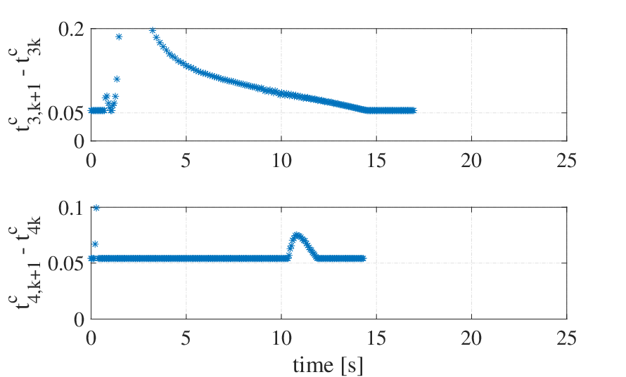
Fig. 2: Consensus of reference models, i=1,⋯,4i=1,\cdots,4.
Refer to caption
Fig. 3: Event-triggered sampling intervals in consensus of reference models.
Refer to caption
Fig. 4: Synchronization profiles of the four agents.
Refer to caption
Refer to caption
Fig. 5: Event-triggered sampling intervals in output regulation.

VI conclusion

In this paper, we have proposed an explicit solution to the event-triggered output synchronization problem for a class of heterogeneous nonlinear multi-agent systems in a network with a directed topology. It has also been shown that continuous monitoring among agents and Zeno phenomenon can be avoided. The two-fold result given in this paper has contributions to development of networked event-triggering mechanisms for both linear systems and nonlinear systems.

References

  • [1] X. Chen and Z. Chen, “Robust perturbed output regulation and synchronization of nonlinear heterogeneous multiagents,” IEEE Transactions on Cybernetics, vol. 46, no. 12, pp. 3111–3122, 2016.
  • [2] L. Zhu, Z. Chen, and R. H. Middleton, “A general framework for robust output synchronization of heterogeneous nonlinear networked systems,” IEEE Transactions on Automatic Control, vol. 61, no. 8, pp. 2092–2107, 2016.
  • [3] D. V. Dimarogonas, E. Frazzoli, and K. H. Johansson, “Distributed event-triggered control for multi-agent systems,” IEEE Transactions on Automatic Control, vol. 57, no. 5, pp. 1291–1297, 2012.
  • [4] D. V. Dimarogonas and K. H. Johansson, “Event-triggered control for multi-agent systems,” in Proceedings of the 48h IEEE Conference on Decision and Control (CDC) held jointly with 2009 28th Chinese Control Conference. IEEE, 2009, pp. 7131–7136.
  • [5] ——, “Event-triggered cooperative control,” in 2009 European Control Conference (ECC). IEEE, 2009, pp. 3015–3020.
  • [6] K. J. Aström and B. Bernhardsson, “Comparison of periodic and event based sampling for first-order stochastic systems,” in Proceedings of the 14th IFAC World congress, vol. 11. Citeseer, 1999, pp. 301–306.
  • [7] D. N. Borgers and W. M. Heemels, “Event-separation properties of event-triggered control systems,” IEEE Transactions on Automatic Control, vol. 59, no. 10, pp. 2644–2656, 2014.
  • [8] E. Garcia, Y. Cao, H. Yu, P. Antsaklis, and D. Casbeer, “Decentralised event-triggered cooperative control with limited communication,” International Journal of Control, vol. 86, no. 9, pp. 1479–1488, 2013.
  • [9] W. Zhu, Z.-P. Jiang, and G. Feng, “Event-based consensus of multi-agent systems with general linear models,” Automatica, vol. 50, no. 2, pp. 552–558, 2014.
  • [10] L. Xing, C. Wen, F. Guo, Z. Liu, and H. Su, “Event-based consensus for linear multiagent systems without continuous communication,” IEEE Transactions on Cybernetics, vol. 47, no. 8, pp. 2132–2142, 2017.
  • [11] Y. Fan, G. Feng, Y. Wang, and C. Song, “Distributed event-triggered control of multi-agent systems with combinational measurements,” Automatica, vol. 49, no. 2, pp. 671–675, 2013.
  • [12] Z. Sun, N. Huang, B. D. Anderson, and Z. Duan, “Comments on Distributed event-triggered control of multi-agent systems with combinational measurements,” Automatica: A journal of IFAC the International Federation of Automatic Control, no. 92, pp. 264–265, 2018.
  • [13] W. Hu, L. Liu, and G. Feng, “Consensus of linear multi-agent systems by distributed event-triggered strategy,” IEEE transactions on cybernetics, vol. 46, no. 1, pp. 148–157, 2016.
  • [14] C. Du, X. Liu, H. Liu, and P. Lu, “Distributed event-triggered consensus control for general linear multi-agent systems under directed graph,” in Decision and Control (CDC), 2017 IEEE 56th Annual Conference on. IEEE, 2017, pp. 4550–4555.
  • [15] Z. Liu, Z. Chen, and Z. Yuan, “Event-triggered average-consensus of multi-agent systems with weighted and direct topology,” Journal of Systems Science and Complexity, vol. 25, no. 5, pp. 845–855, 2012.
  • [16] C. Nowzari and J. Cortés, “Distributed event-triggered coordination for average consensus on weight-balanced digraphs,” Automatica, vol. 68, pp. 237–244, 2016.
  • [17] G. S. Seyboth, D. V. Dimarogonas, and K. H. Johansson, “Event-based broadcasting for multi-agent average consensus,” Automatica, vol. 49, no. 1, pp. 245–252, 2013.
  • [18] A. Girard, “Dynamic triggering mechanisms for event-triggered control,” IEEE Transactions on Automatic Control, vol. 60, no. 7, pp. 1992–1997, 2015.
  • [19] Z. Sun, N. Huang, B. D. Anderson, and Z. Duan, “A new distributed zeno-free event-triggered algorithm for multi-agent consensus,” in Decision and Control (CDC), 2016 IEEE 55th Conference on. IEEE, 2016, pp. 3444–3449.
  • [20] X. Meng and T. Chen, “Event based agreement protocols for multi-agent networks,” Automatica, vol. 49, no. 7, pp. 2125–2132, 2013.
  • [21] G. Guo, L. Ding, and Q.-L. Han, “A distributed event-triggered transmission strategy for sampled-data consensus of multi-agent systems,” Automatica, vol. 50, no. 5, pp. 1489–1496, 2014.
  • [22] M. Mazo and P. Tabuada, “Decentralized event-triggered control over wireless sensor/actuator networks,” IEEE Transactions on Automatic control, vol. 56, no. 10, pp. 2456–2461, 2011.
  • [23] P. M. Tallapragada and N. Chopra, “Decentralized event-triggering for control of nonlinear systems,” IEEE Transactions on Automatic control, vol. 59, no. 12, pp. 3312–3324, 2014.
  • [24] Y. Fan, L. Liu, G. Feng, and Y. Wang, “Self-triggered consensus for multi-agent systems with zeno-free triggers,” IEEE Transactions on Automatic Control, vol. 60, no. 10, pp. 2779–2784, 2015.
  • [25] W. Hu, L. Liu, and G. Feng, “Output consensus of heterogeneous linear multi-agent systems by distributed event-triggered/self-triggered strategy,” IEEE transactions on cybernetics, vol. 47, no. 8, pp. 1914–1924, 2017.
  • [26] W. Xu, D. W. Ho, L. Li, and J. Cao, “Event-triggered schemes on leader-following consensus of general linear multiagent systems under different topologies,” IEEE Transactions on Cybernetics, vol. 47, no. 1, pp. 212–223, 2017.
  • [27] T. Liu and Z.-P. Jiang, “A small-gain approach to robust event-triggered control of nonlinear systems,” IEEE Transactions on Automatic Control, vol. 60, no. 8, pp. 2072–2085, 2015.
  • [28] ——, “Event-based control of nonlinear systems with partial state and output feedback,” Automatica, vol. 53, pp. 10–22, 2015.
  • [29] W. Liu and J. Huang, “Event-triggered global robust output regulation for a class of nonlinear systems,” IEEE Transactions on Automatic Control, vol. 62, no. 11, pp. 5923–5930, 2017.
  • [30] ——, “Cooperative global robust output regulation for a class of nonlinear multi-agent systems by distributed event-triggered control,” Automatica, vol. 93, pp. 138–148, 2018.
  • [31] J. Wang, A. Sheng, D. Xu, Z. Chen, and Y. Su, “Event-based practical output regulation for a class of multiagent nonlinear systems,” IEEE transactions on cybernetics, no. 99, pp. 1–10, 2018.
  • [32] G. D. Khan, Z. Chen, and L. Zhu, “A new approach for event-triggered stabilization and output regulation of nonlinear systems,” IEEE Transactions on Automatic Control, p. Submitted, 2018.
  • [33] Z. Chen and H. Fujioka, “Performance analysis of nonlinear sampled-data emulated controllers,” IEEE Transactions on Automatic Control, vol. 59, no. 10, pp. 2778–2783, 2014.
  • [34] J. Mei, W. Ren, and J. Chen, “Consensus of second-order heterogeneous multi-agent systems under a directed graph,” in American Control Conference (ACC), 2014. IEEE, 2014, pp. 802–807.
  • [35] V. Kucera, “A contribution to matrix quadratic equations,” IEEE Transactions on Automatic Control, vol. 17, no. 3, pp. 344–347, 1972.
  • [36] Z. Chen and J. Huang, Stabilization and regulation of nonlinear systems. Springer, 2015.