Precise Radial Velocities of Cool Low Mass Stars With iSHELLishell_reduction (https://github.com/jgagneastro/ishell_reduction), PySHELL (Available upon request), Scipy (Jones et al. 2001), Matplotlib, (Hunter 2007), barycentric vel.pro (Wright & Eastman 2014)
Abstract
The coolest dwarf stars are intrinsically faint at visible wavelengths and exhibit rotationally modulated stellar activity from spots and plages. It is advantageous to observe these stars at near infrared (NIR) wavelengths (1-2.5 µm) where they emit the bulk of their bolometric luminosity and are most quiescent. In this work we describe our methodology and results in obtaining precise radial velocity (RV) measurements of low mass stars using K-band spectra taken with the R~80,000 iSHELL spectrograph and the NASA Infrared Telescope Facility (IRTF) using a methane isotopologue gas cell in the calibration unit. Our novel analysis pipeline extracts RVs by minimizing the RMS of the residuals between the observed spectrum and a forward model. The model accounts for the gas cell, tellurics, blaze function, multiple sources of quasi-sinusoidal fringing, and line spread function of the spectrograph (LSF). The stellar template is derived iteratively using the target observations themselves through averaging barycenter-shifted residuals. We have demonstrated 5 ms-1 precision over one-year timescales for the M4 dwarf Barnard’s Star and K dwarf 61 Cygni A, and 3 ms-1 over a month for the M2 dwarf GJ 15 A. This work demonstrates the potential for iSHELL to determine dynamical masses for candidate exoplanets discovered with the NASA TESS mission, and to search for exoplanets orbiting moderately active and/or young K & M dwarfs.
Keywords:
atmospheric effects, infrared: stars, methods: data analysis, stars: individual (61 Cygni A, Barnard’s Star, GJ 15 A), techniques: radial velocitiesI Introduction
The radial velocity (RV) technique has been successfully applied to reveal hundreds of systems around solar-type (FGK dwarf) stars since the discovery of 51 Pegasi b in 1995 (Mayor & Queloz 1995). Observations are usually performed at visible wavelengths where these stars are brightest and telluric lines are relatively scarce (Plavchan et al. 2015; Fischer et al. 2016). However, 75% of the stars in the solar neighborhood are cooler, less luminous M dwarfs (RECONS 2018). The “habitable zone” around M dwarfs is much closer to the star due to their lower luminosities, significantly shortening the timescales needed to detect habitable zone worlds. The lower stellar mass also means a larger reflex velocity for a given planet mass. These advantages have been recently exploited in the discovery of the planet in the habitable zone of the M dwarf Proxima Cen (Anglada-Escudé et al. 2016).
RV observations of M dwarfs, especially mid- to late-type M dwarfs (M4+), are more challenging than those of solar-type stars. M Dwarfs are intrinsically faint and require long integration times per epoch to acquire sufficient SNR, especially for spectroscopic observations where light is dispersed. Late M dwarfs are more magnetically active (West et al. 2004; Basri et al. 2010). Star spots and other sources of activity can introduce RV noise and spurious signals at periods corresponding to the stellar rotation period and harmonics where n is a small integer (Robertson et al. 2015). A further realization for M1-M4 dwarf stars is the stellar rotation period overlaps with the range in periods of habitable zone worlds (Newton et al. 2016; Vanderburg et al. 2016).
Due to the difficulties of RV observations of M dwarfs in the optical, interest has grown in the last decade in developing near-infrared (NIR) spectrographs for these observations. M dwarfs are brightest at near-infrared (NIR) wavelengths, and the flux contrast between star spots and the surrounding chromosphere is reduced (Martín et al. 2010; Mahmud et al. 2011; Crockett et al. 2012; Anglada-Escudé et al. 2013; Marchwinski et al. 2015). To first order in wavelength, the flux contrast (and thus RV signal) from activity is expected to follow a relationship, although additional challenges arise from the wavelength dependence of limb-darkening and convective blue-shift (Reiners et al. 2010). NIR RV efforts have made rapid progress in precision (and thus mass detection) capabilities. NIRSPEC on Keck (K-band, R~25000) obtained 45 ms-1 precision observing late M dwarfs (Tanner et al. 2012). CSHELL (K-band, R~46,000) on IRTF obtained 35 ms-1 observing GJ 15 A (Gao et al. 2016). NIR RV efforts have gained traction both with absorption gas cells (Bean et al. 2010, e.g.) and the use of fiber-feeds to stabilized environments for instruments. As a recent example, the Habitable Zone Planet Finder (HPF) on the 10 meter Hobby-Eberly Telescope (R~50,000, Y- and J-bands) has shown 3 ms-1 precision on Barnard’s Star, sufficient to detect rocky worlds in the habitable zone of M dwarfs (Metcalf et al. 2019a; Metcalf et al. 2019b).
Most NIR RV instruments exploited the , , and regions of the spectrum, although RV information content in the Y- and J-band is found to be lower than expected from synthetic spectra (Reiners et al. 2018). The K-band spectra of M dwarfs also contains deep sharp lines of CO at µm suitable for RV measurements. However, observations in this wavelength region are also plagued with telluric lines of water and methane as well as other trace molecules that complicate the data analysis (Seifahrt et al. 2010).
In this paper, we describe our methodology in obtaining precise NIR RVs from observations of cool low mass stars using the iSHELL spectrograph (Rayner et al. 2016) on the 3 meter NASA Infrared Telescope Facility (IRTF) at K-band wavelengths (2.18-2.47 ). We present our novel pipeline extending the work of Gao et al. 2016 with CSHELL in Sections III and IV. We test our pipeline with observations of Barnard’s Star (GJ 699), GJ 15 A, and 61 Cygni A, all previously used in RV searches and suitable as RV standards, and present the results in Section V. We analyze the fidelity of our stellar template retrieval in Section VI, and forward model parameter distributions in Section VII. In Section VIII we discuss our particular choice of forward model and how our obtained iSHELL RV precision compares to other precise NIR spectrographs, as well as prospects for planet confirmation. A summary of this work is provided in Section IX.
II Observations
We obtained spectra with the iSHELL spectrograph on the 3 meter NASA Infrared Telescope Facility (IRTF) between October 2016 and October 2017, with the majority of observations taking place during the first half of this period. Table 2 provides the estimated SNR (per detector pixel) of each observation as well as the number of observations (N) obtained each night. Spectra are recorded using the iSHELL spectrograph in KGAS mode (2.18-2.47 ) with a 0.375” slit at R~80,000. A Hawaii 2RG array records 29 cross-dispersed echelle orders () spanning this spectral range. A methane isotopologue () gas cell in the calibration unit with 90% continuum throughput is used to provide a common optical path wavelength reference and to constrain the variable line spread function (LSF) of the spectrograph (Anglada-Escudé et al. 2012; Plavchan et al. 2013). To minimize errors in the barycenter correction and telluric optical depths of individual spectra, integration times are limited to 5 minutes. The exposure midpoint (opposed to flux-weighted) is used to determine the barycentric correction since iSHELL does not have an exposure meter as is common in visible precise RV instruments (Wright & Eastman 2014). Unfortunately, the error in barycenter correction scales with square of the exposure time (Tronsgaard et al. 2019), so doubling an exposure time will quadruple our barycenter velocity uncertainty. Various factors can further contribute to a non-constant photon rate, particularly changes in airmass and atmospheric transparency. The telluric content (particularly water) can be variable on time-scales of an hour or less along with the changing airmass of our target (Sameshima et al. 2018), so we limit our maximum exposure time to avoid any errors that could potentially be introduced in the telluric modeling, although we do not characterize this. We further limit integration times to avoid the nonlinear detector regime of the detector for brighter targets. After every target is observed, a set of five flat-fields is obtained before slewing the telescope to the next target. An example of a raw unprocessed 2-dimensional fits image is shown in Fig. 1. All data are available online at the NASA/IPAC Infrared Science Archive.11 1 Available at https://irsa.ipac.caltech.edu/applications/irtf/. All IRTF data has a proprietary period of 18 months starting at the end of that observing semester.
We choose three bright RV standards to evaluate the RV precision obtainable with iSHELL. These targets have already been observed to show RV stability at or below the expected iSHELL precision, and are summarized in Table 1. Barnard’s Star (GJ 699) shows no RV variations down to 2 ms-1 over several years using data sets from Keck/HIRES & Lick/Hamilton after accounting for the observed secular acceleration of 4.515 ms-1yr-1 (Choi et al. 2012). More recent efforts have found a low-amplitude periodic signal at 233 days and ms-1 (Ribas et al. 2018). 61 Cygni is a binary system of two comparatively bright K dwarfs with an orbital period of 653 years, neither of which are known to host any planets. GJ 15 A is suspected to host a single planet with ms-1 and a period of 11.44 days (Howard et al. 2014).
| Star | R.A./Decl. | Spec. Type | Planets | Reference | |
|---|---|---|---|---|---|
| GJ 699 |
17:57:48.5
+04:41:36.1 |
M4V | 4.52 | b: ms-1, P=233 days |
Jenkins et al. 2009
Ribas et al. 2018 |
| GJ 15 A |
00:18:22.9
+44:01:22.6 |
M2V | 4.02 | b: ms-1, P=11.4 days |
Jenkins et al. 2009
Howard et al. 2014 |
| 61 Cygni A |
21:06:53.9
+38:44:57.9 |
K5V | 2.68 | No known planets | van Belle & von Braun 2009 |
| UT Date | Int. Time | a | b | |
| —Barnard’s Star— | ||||
| 2016 Oct. 16 | 4 | 5 min | 139 | 277 |
| 2016 Oct. 23 | 7 | 5 min | 159 | 420 |
| 2016 Nov. 06 | 8 | 5 min | 146 | 413 |
| 2016 Nov. 07 | 4 | 5 min | 201 | 402 |
| 2017 Apr. 06 | 9 | 5 min | 132 | 397 |
| 2017 Jun. 18 | 6 | 5 min | 164 | 402 |
| 2017 Jun. 26 | 6 | 5 min | 160 | 392 |
| 2017 Jul. 05 | 7 | 5 min | 152 | 402 |
| 2017 Jul. 29 | 10 | 5 min | 133 | 420 |
| 2017 Oct. 20 | 16 | 20 sec | 41c | 164c |
| 2017 Oct. 21 | 16 | 20 sec | 41c | 164c |
| 2017 Oct. 22 | 16 | 20 sec | 41c | 164c |
| 2017 Oct. 23 | 16 | 20 sec | 41c | 164c |
| —GJ 15 A— | ||||
| 2016 Oct. 16 | 7 | 2.5 min | 198 | 525 |
| 2016 Oct. 17 | 12 | 2.5 min | 150 | 521 |
| 2016 Oct. 22 | 8 | 2.5 min | 179 | 505 |
| 2016 Oct. 23 | 17 | 2.5 min | 122 | 503 |
| 2016 Nov. 06 | 16 | 1.5 min | 127 | 506 |
| 2016 Nov. 07 | 11 | 2.5 min | 158 | 524 |
| —61 Cygni A— | ||||
| 2016 Oct. 16 | 10 | 30 sec | 170 | 537 |
| 2016 Oct. 17 | 12 | 1 min | 152 | 525 |
| 2016 Oct. 22 | 23 | 15 sec | 105 | 502 |
| 2016 Oct. 23 | 10 | 1 min | 162 | 513 |
| 2016 Nov. 06 | 6 | 1 min | 127 | 506 |
| 2016 Nov. 07 | 16 | 15 sec | 126 | 502 |
| 2017 Apr. 06 | 7 | 1.5 min | 194 | 514 |
| 2017 Apr. 12 | 6 | 1.5 min | 210 | 515 |
| 2017 Jun. 18 | 5 | 1.5 min | 258 | 577 |
| 2017 Jun. 26 | 6 | 1.5 min | 223 | 546 |
| 2017 Jul. 05 | 11 | 1.5 min | 154 | 510 |
- a
represents the SNR per spectral pixel for an individual spectrum measured by summing the area of a Gaussian PSF model to the data near the blaze peak with no spectral features with the iSHELL observing gui. Sky noise is not used in this estimation.
- b
represents the total (co-added) SNR per spectral pixel for a consecutive series of observations, with .
- c
SNR was not recorded during the last four observations for Barnard’s Star and are an estimation from the previous nights assuming a relationship of SNR .
III Data Reduction
We reduce iSHELL data with custom Interactive Data Language (IDL) software routines22 2 Available at https://github.com/jgagneastro/ishell_reduction; version 1.1 and commit number dc5367c93d4ee37ae72286cf338388a2a9727155 were used.. For each nightly target, we locate the spectral trace using the corresponding flat-fields. We generate a master flat field which is free of sinusoidal fringing through various smoothing techniques. We then divide the corresponding science data by this master flat to correct for the slit illumination and pixel-to-pixel response. We finally iteratively extract the 1-dimensional spectral orders through an iterative process where we obtain a better estimation of the spatial point spread function (PSF), spectral flux density, and identification of bad pixels with each iteration.
First, we median combine and use the flat-fields to detect the 29 echelle order traces. We model the edges and center of each order with independent second-degree polynomials. In each flat-field order, we straighten the order into a rectangular array by linear interpolation in the spatial direction. We smooth in the spectral direction using a 45-pixel rolling median. We then divide the straightened flat by the spectrally-smoothed flat to isolate instrumental fringing in the flat-field (See Section IV.2.1). A one-dimensional version of the fringing is then obtained by taking the vertical median in the spatial direction, and smoothing the resulting 1-dimensional array with a 3-pixel rolling median. We divide the fringing pattern in each order to finally remove the fringing present in the flat-fields (Fig. 2).
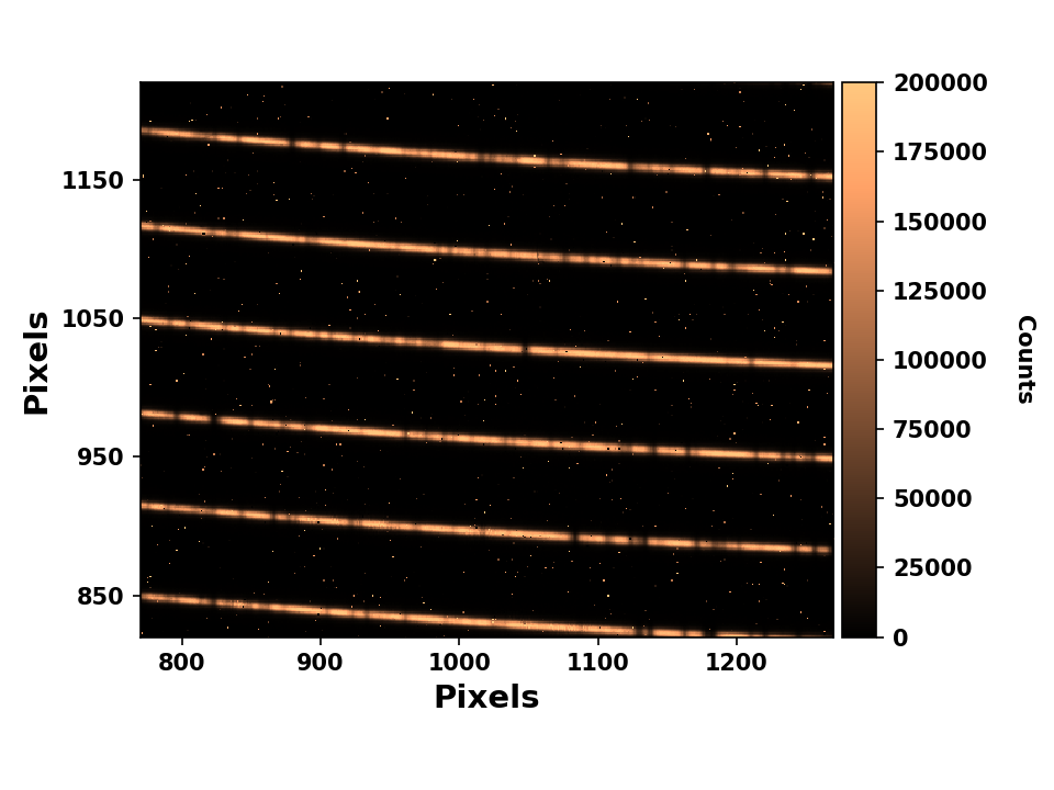


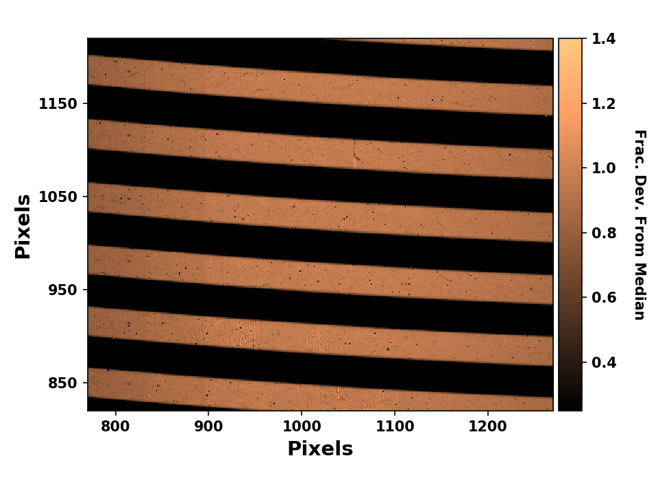
Next we divide the corrected flat-field into all individual science exposures to correct the slit illumination and pixel-to-pixel response function without injecting an additional fringing pattern in the science exposures. The fringing in iSHELL is not stable in phase and amplitude, nor is the slit-illumination function identical between flat-field (quartz lamp) and stellar (point) sources, and thus does not perfectly divide out if left in the flat-fields.
To extract the spectra, we use a multi-step iterative process. First, we straighten the individual spectral orders of each science exposure with the corresponding order’s central position polynomial (from the flat-fields). For each order, an initial (spatial) point spread function is constructed using a median filter in the dispersion (wavelength) direction. A first spectral extraction is performed by using the estimated point spread function as an extraction weight on the rectified order. A cross-correlation of the estimated profile with the straightened data is next performed at each spectral position where the estimated spectral flux density is above half of a cutoff value, set at the 80% quartile value of the spectral flux density. This results in a more precise trace position of the data within each order, which is next modeled with a second-degree polynomial.
We next create a curved two-dimensional spectral profile from the spatial point spread function and refined second-degree polynomial of the science trace position. We obtain a better estimate of the spectral flux density and avoid interpolation by using this two-dimensional profile as an extraction weight on the non-straightened science order. Significant outliers in the resulting spectral flux density are also masked iteratively by flagging large deviations taking place within less than three spectral pixels.
Next, this cleaned up version of the spectral flux density is used in combination with the two-dimensional trace to build a clean version of the two-dimensional science trace. Dividing the science trace by this resulting image allows us to flag bad pixels directly in the two-dimensional data by looking at significant outliers in flux deviations that happen within three pixels. This allows us to mask the deviant pixels directly in the two-dimensional image and to refine our best estimate of the spectral flux density by performing an optimal (maximum SNR) extraction (Horne 1986) using the masked two-dimensional spectral trace and the curved two-dimensional point spread function.
As a final step to refine the spectral flux density, we allow the width of the spatial line profile to vary linearly in the spectral direction within each order. To do this required modeling the spatial point spread function; we found that a Gaussian profile represents the data adequately. A Gaussian profile is fit at each spectral position of the masked two-dimensional science trace, and the resulting Gaussian profile width versus spectral pixel position is fit with a first-degree polynomial. This is used to build a final version of the curved two-dimensional extraction profile, and a last optimal extraction is performed with this profile to obtain our final extracted spectral flux density. Examples of reduced spectra are shown in Figs. 3 & 4.


IV Radial Velocity Pipeline
In this section, we describe the methods used to extract RVs by forward modeling single-order extracted (one-dimensional) science spectra (IV.2–IV.3), then compute nightly RV measurements and finally optimize multi-order RVs in Section IV.4. We adapt the RV pipeline for CSHELL spectra described in Gao et al. 2016 to iSHELL data. We have rewritten the CSHELL code in a Python script PySHELL33 3 Available upon request. taking into account iSHELL’s larger spectral grasp with multiple orders. Due to variability in the blaze function and due to the lower SNR, we choose to ignore the first and last 200 pixels at the edges of the 2048-element extracted spectra. Utilizing the remaining pixels is a subject of future work. Our radial velocity pipeline represents a significant departure from traditional analyses with iodine cell data. Rather than splitting orders into smaller chunks and introducing discontinuities at the boundaries, we model entire orders as a single “chunk”. This necessitates a more complex forward model than is used with traditional iodine cells (e.g. Butler et al. 1996).
IV.1 Choice of Numerical Solver
To fit a model to the extracted one-dimensional spectra, we have implemented a custom downhill Nelder-Mead algorithm that performs simplex calls for the entire parameter space followed by consecutive two-dimensional subspace calls for all neighboring pairs of parameters to better handle the large dimensional space, as standard Nelder-Mead algorithms fail to converge. A similar approach that we did not test would be to: first use SciPy’s optimize routine with method=Nelder-Mead a single time for the entire parameter space; second use optimize for each consecutive pair of parameters keeping others constant ; and finally third, repeat the first two steps for the number of parameters in the model. The minimum RMS is continuously improved with each call to optimize as the parameters converge. Our algorithm is therefore dependent on the parameter ordering, and we do not explore the impact of parameter ordering in this work. However, the RMS typically converges before iterations of the algorithm. Our specific Nelder-Mead algorithm in Python for a given simplex is based on that used for CSHELL given by Bajzer & Penzar 1999 but with stricter convergence requirements. Specifically, the largest fractional difference in the RMS for the current simplex must be less than three times in a row for the solver to be considered successfully converged.
IV.2 Spectral Forward Model
For a given echelle order, we define the forward model intensity as
| (1) |
where * represents a convolution. We describe each of the forward model terms in turn. is the Doppler shifted stellar spectrum derived iteratively and described in detail in Section IV.3. is our gas cell spectrum, obtained with a Fourier Transform Spectrometer (FTS) at the NASA Jet Propulsion Laboratory (JPL) at R~500,000 (Anglada-Escudé et al. 2012; Plavchan et al. 2013). Like Gao et al. 2016, we find the gas cell optical depth (vs. unity) because of the off-axis angle the gas cell was placed in the FTS, as opposed to CSHELL & iSHELL where the path length is minimized. corresponds to the Doppler shifted telluric absorption spectrum with optical depth . For KGAS mode, the relevant telluric components are water (), methane (), nitrous oxide (), and carbon dioxide (). Each component is obtained from Transmissions of the AtmosPhere for AStromomical data (TAPAS) (Bertaux et al. 2014). We use realistic temperature-pressure profiles for Maunakea corresponding to the zenith and date of April 12, 2018 at midnight (arbitrarily chosen). The telluric shift is common to all species, but each can have different optical depths to account for variable atmospheric content. The stellar and telluric shifts are computed on a logarithmic grid keeping If a telluric component has no absorption features prior to convolution, it is excluded from the fit for that order. The effective resolution of the gas cell and telluric templates in our spectral model are 5 and 15 times that of the data, respectively.
is the residual blaze function left over after the flat division in data reduction. The residual blaze is relatively consistent across orders for a sequence of observations, and is approximately quadratic. While the deviations from the quadratic are not well-modeled with an analytic function, they are relatively small in flux ( 10%). We first model the blaze with a quadratic to approximate the general curvature of the continuum, then use 14 cubic splines as an additive correction. A wavelength grid for the blaze function spline correction is generated by first starting from an initial guess for the wavelength solution. The corresponding grid for each spline point is then generated using a linearly spaced array with endpoints corresponding to the estimated wavelengths of pixels 200 and 1848 (the cropped data) with an extra padding of 0.1nm to account for the error in the initial wavelength solution, ensuring that no spline points are outside of the cropped data.
LSF represents the line spread function (line profile) of the spectrograph and is constructed using a sum of Gaussians with Hermite polynomial coefficients (Arfken G. 2012). These are derived iteratively using
| (2) | |||
| (3) |
where with being the Gaussian width of . The LSF is then constructed by summing over ,
| (4) |
where is the highest order of the Hermite function series. We use (up to ), and explore other LSF models in Section VIII.2. The LSF is normalized as a final step. Further, the convolution is only performed within a window of nm for the model pixel as convolution is computationally expensive.
Like the residual blaze function, we compute the wavelength grid of the data, for pixels , via a main quadratic component, plus a cubic spline correction for small local deviations. Unlike the blaze, a need for splines here is not initially obvious. As discussed further in Section VIII.1, however, inclusion of a spline correction in the wavelength solution improves the resulting RVs. To obtain the main quadratic component for the wavelength solution, pixel (from blue to red) is mapped to a window nm. An initial guess for the zero points are predetermined from modeling several nights of Vega data with no stellar lines. From here, the polynomial coefficients are determined through a matrix inversion and a quadratic wavelength solution is obtained for all pixels. While are not orthogonal parameters, we find that polynomial coefficients yield similar RV precision, and opt to use these “Lagrange points” for their simple behavior. Wavelength splines are placed on top of the quadratic by first choosing evenly spaced pixels (for the cropped data) equal to the number of splines plus one. Each pixel gets mapped to the range nm and are interpolated onto the data pixel grid using cubic spline interpolation. The sum of the quadratic and spline correction yields the final wavelength solution for a given spectrum.
IV.2.1 Fringing
and represent the two sources of fringing present in iSHELL data. The first is introduced by the order selection (OS) filter, before the light is diffracted at the echelle grating44 4 Upgrades planned for late 2019 will replace the order selection filter with a wedged version to eliminate this source of fringing in iSHELL spectra (Rayner, private comm.).. The OS filter behaves as a Fabry-Perót cavity, introducing a sinusoidal-like pattern with an amplitude of a few percent, and is modeled by:
| (5) | |||
| (6) |
is the amplitude of the signal and traces the optical path length through the cavity. corresponds to the finesse of the cavity, where R is the reflectance (Lipson S.G. 1995). A large finesse manifests as sharper downward cavity absorption spikes for the sinusoid, but we don’t see significant evidence for a large cavity finesse for in our data. Varying reveals no obvious preference for any particular value and solutions settle at both upper and lower bounds (0.1, 2) and shows no significant improvement in RVs, so we force .
The second source of fringing is introduced by the anti-reflective (AR) coating of the silicon immersion grating surface on the echelle as the light exits the grating. It is modeled with a similar Fabry-Perót absorption equation, but in a more complex form because of the wavelength-dependent angle of the incidence on the cavity:
| (7) |
and are geometric properties of the immersion grating and assumed constant. again traces the optical thickness of the cavity, and allows for a phase shift. corresponds to the wavelength with the shortest orthogonal path through the AR cavity with . We further opt to replace with a second wavelength “set point” corresponding to an overall phase of , where 68 is arbitrarily chosen to span a significant fraction of the order. , and are free parameters, along with the amplitude and finesse . A detailed derivation of this equation will be presented in Cale et al. (in prep).
Eq. 7 deviates from the standard fringing equation because the incident light at the AR exit face has already been diffracted at the echelle and is therefore spatially separated as a function of , resulting in different resonant cavity lengths for different wavelengths as they enter the AR cavity at different angles (Fig. 5). The AR fringing component has noticeably sharp downward cavity absorption features, indicating a large finesse, so we fit for . Lastly, we multiply the model by after convolution because it’s introduced post-diffraction. One signal we do not observe in our data is fringing corresponding to interference when light enters the AR cavity before getting diffracted at the echelle. We expect this would induce a signal similar to that of the OS filter with a corresponding amplitude and value for . A summary of all forward model parameters is given in Table 3.

| Num. | Description [units] | Symbol | Value/Bounds |
|---|---|---|---|
| 1 | Stellar Doppler Shift [ms-1] | unbounded | |
| 2 | Gas Cell Optical Depth | 0.97 | |
| 3 | Telluric Doppler Shift [ms-1] | (-200, 200) | |
| 4 | Optical Depth | (0.02, 4.0) | |
| 5 | Optical Depth | (0.1, 3.0) | |
| 6 | Optical Depth | (0.05, 3.0) | |
| 7 | Optical Depth | (0.05, 3.0) | |
| 8 | OS Filter Fringing Amplitude | (0.015, 0.043) | |
| 9 | OS Filter Fringing Cavity Length Scale [nm] | (, ) | |
| 10 | OS Filter Fringing Finesse | 1.0 | |
| 11 | AR Fringing Amplitude | (0, 0.03) | |
| 12 | AR Fringing Reflection Point [nm] | 0.075 | |
| 13 | AR Fringing Set Point [nm] | 0.05 | |
| 14 | AR Fringing Phase | (0, 2) | |
| 15 | AR Fringing Finesse | (1, 4) | |
| 16 | Immersion Grating Tilt Angle | 71.57097° | |
| 17 | Blaze Angle | 71.56795° | |
| 18-20 | Wavelength Solution Lagrange Points (3 total) [nm] | 0.05 | |
| 21 | Blaze Function Quadratic Term | (, ) | |
| 22 | Blaze Function Linear Term | (, ) | |
| 23 | Blaze Function Order Term | (0.98, 1.08) | |
| 24 | LSF Width [Model pixels] | (5.5, 12) | |
| 25-30 | LSF Hermite Terms (6 total) | 0.4 | |
| 31-45 | Blaze Spline Lagrange Point (15 total) | 0.135 | |
| 46-52 | Wavelength Solution Spline Lagrange Points (7 total) [nm] | 0.0125 |
IV.3 Stellar Template Retrieval
The derivation of the unconvolved stellar spectrum has consistently proven to be a difficult step in forward modeling spectra, particularly in the NIR (Bean et al. 2010). One approach is to use synthetic model spectra instead. Models of stellar atmospheres can produce synthetic stellar spectra given the effective temperature, metallicity, and surface gravity (Blake et al. 2010; Crockett et al. 2011; Bailey et al. 2012; Tanner et al. 2012). Due to their lower effective temperatures, atmospheres of late M dwarfs (and brown dwarfs) contain molecular ro-vibrational transitions which can which can significantly contribute to the opacity and affect the emitted spectrum at certain wavelengths (Allard et al. 2003). While the addition and refinement of molecular opacities and full 3D radiation transfer in newer models (such as the BT-Settl PHEONIX models) are providing a better match with observations (Allard et al. 2011), there are still some deficiencies.
A second approach is to deconvolve spectra of A or B stars with little to no stellar spectral features observed through an absorption gas cell (e.g iodine). Spectral lines from the gas cell (and tellurics) provide a means of obtaining the line profile (LSF) of the spectrograph, and this can be used to deconvolve the spectrum of a science target taken just before or soon after at a similar airmass and direction in the sky. However this approach presumes the LSF remains stable between observations. This may be true for instruments relying on stabilization, but may not be the case for iSHELL as it slews with the telescope at the Cassegrain focus.
We therefore choose to rely on the target observations themselves to extract the stellar spectrum using an iterative deconvolution method described in Sato et al. 2002. If is the only unknown variable in the model, then the residuals from a model using an imperfect stellar template correspond to the missing (or extra) features of the stellar template, up to a convolution and Doppler shift. Furthermore, by averaging together many spectra, the coadded signal-to-noise is much higher than in individual spectra. In the limit of iteratively adding the residuals back to the stellar template, the template approaches the unconvolved spectrum. This iterative deconvolution method does have its own limitations. First, sufficient sampling at multiple barycenter velocities with high combined SNR are necessary (e.g. two RV data points are not enough). Second, residual correlated noise can gradually get repeatedly added into the stellar template from missed bad pixels, or from non-stellar spectral features that are not well fit.
In our work, we start with a flat guess for and forward model all spectra. We choose a forward model wavelength grid resolution that is about 8 times the data spectral resolution to oversample the data and LSF. Higher resolution models yield similar RV precision and RMS values. To compare the model to the observed spectrum (compute an RMS), the high resolution model is linearly interpolated onto the lower-resolution data grid. We shift each set of residuals to a pseudo rest frame of the star according to the barycenter corrections () obtained from barycentric_vel.pro55 5 Available at http://astroutils.astronomy.ohio-state.edu/exofast/ (Wright & Eastman 2014), decoupling stellar features from any coherent features in the rest frame of the gas cell. We interpolate residuals onto the high resolution model wavelength grid using cubic splines and then median combine across spectra, weighted by RMS-2 of the residuals from the forward model fit. We add the median values to the previous template, and re-fit the spectra. We repeat this process until the RVs stabilize, which happens anywhere between 5-40 iterations for orders low in RV content, but typically at later iterations for orders high in RV content. We run all targets through 41 iterations to assess convergence and RV precision.
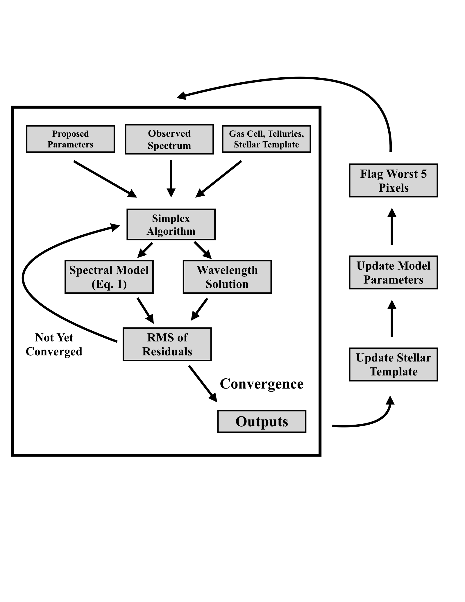
Furthermore, we run the flat template twice on the “first” iteration, where we attempt to minimize the effect of the deep stellar CO lines on the solver by masking values deeper than in the residuals of the first attempt. The blaze function splines and AR fringing are not well-constrained in the presence of poorly fit stellar lines, and are not included in the first iteration. We do not assess the impact of the initial error in the blaze on the RVs and stellar template generation at later iterations. However, with the variation in phase and decoupling from the star, any fringing that survives the weighted median combination in the pseudo rest frame of the star is minimized. We also force max{} 1, as the continuum is not well-constrained in early iterations. This requirement may be loosened at later iterations, although this is not explored in this work. Lastly, on iteration 10 and each iteration thereafter, we flag the worst 5 pixels in each set of residuals (see Fig. 7). After 41 iterations, this flags nearly 10% of all originally used pixels (150 of ~1648), but improves RV precision at later iterations. Each iteration produces a Doppler shift for each individual spectrum. To calculate an individual relative RV, we “subtract” off the barycenter correction from the full Doppler shift, . An outline of the forward model is given in Fig. 6.
After each iteration for a given order, we output text files and corresponding figures for the:
- •
Best fit model to the data and corresponding parameters.
- •
Wavelength solution to the data.
- •
Flagged (ignored) pixels.
- •
The stellar template used for this iteration.
- •
Individual and co-added nightly RVs.
- •
Residuals between the data and models with flagged pixels marked as zeros and the corresponding RMS values and number of target function calls.
To forward model our spectra in a timely manner, we use the ARGO cluster provided by the Office of Research Computing at George Mason University, VA, which can designate 280 cores to a single user, and the exo cluster at George Mason University, currently with 84 cores. Forward modeling a single-order spectrum takes 5-15 minutes at early iterations per core, but only 1-5 minutes at later iterations as parameters have already converged from their updated initial guess.
IV.4 RV Calculations
We explore two methods for computing one radial velocity measurement for each night averaged across echelle orders. The first extends on Gao et al. 2016 utilizing a series of weighted statistical formulas (Section IV.5). We also explore a second approach which numerically solves for the relative “zero-points” for each echelle order (Section IV.6).
IV.5 Weighted Statistics
In the equations that follow, & correspond to the night, individual observation, data pixel, and echelle order, respectively. In order to minimize our RV error per epoch, individual observations at are co-added to obtain a measurement at (see Table 2), weighted by RMS-2 from the forward model fit:
| (8) | |||
| (9) |
where and are the individual RVs and weights for order m, respectively. corresponds to the number of observations for the night. and are the observed and model spectra, respectively, computed at the data pixel. is the number of used pixels for the observation for order (e.g. ~1648–flagged pixels). Deviant pixels flagged during data reduction or forward modeling are not included in the sum.
Nightly error bars are computed via an unbiased weighted standard deviation, divided by the square root of the number of spectra used for that night, .
| (10) |
Before RVs from different echelle orders are combined, the weighted average RV of each order is subtracted off. Combined nightly RVs are then computed through a second weighted average,
| (11) | |||
| (12) | |||
| (13) | |||
| (14) |
where is the number of echelle orders used.
IV.6 Detrending Minimization
Second, to better constrain the intrinsic order dependent characteristic RVs (assumed to be above), we utilize a version of the Trend Filtering Algorithm (TFA) (Kovács et al. 2005) which is frequently used to remove systematics and detrend Kepler light curves (Aigrain et al. 2017; Still & Barclay 2012). We implement and minimize a modified weighted formula from Bedell et al. 2019 akin to the weighted implementation of TFA in Gopalan et al. 2016:
| (15) |
are the nightly RVs from Eq. 8, are the new order offsets, and are the “detrended” RVs for the night. and are sets of free parameters with lengths and , respectively. The weighted average of each order from Eq. 11 is still subtracted from before optimizing. Values of and are set to zero as an initial guess with bounds 5 ms-1 and 50 ms-1, respectively. Final error bars are computed using Eq. 13 with the detrended orders, . The parameters are optimized using the same Nelder-Mead algorithm described in Section IV.1.
V Results
For each of the three stars, we run orders through 41 iterations. Order numbers contain sufficient stellar and gas cell RV information content, but are also higher in water absorption and haven’t yielded comparable RV precision (30 ms-1 long-term). We aim to explore a more sophisticated telluric model for these orders in future work. Higher order numbers shortward of the CO band () are relatively low in stellar RV content and have fewer gas cell lines for a precise wavelength calibration (see Section V.2).
For Barnard’s Star, we also compute RVs separately from the first nine nights for orders , which we refer to as the “high SNR run” in the rest of this paper. Barnard’s Star has historically been shown to have the highest long-term RV stability with precisions below our expected noise floor, so we use it to assess multi-order RV precision (Section V.1), forward model parameter distributions (Section VII) and alternative forward model implementations (Section VIII). This also shows the impact of including lower SNR observations in the stellar template generation. Fig. 7 shows example fits of the model spectrum to a high and low SNR observation of Barnard’s Star. The residuals (and thus RMS) for the low SNR observations are typically twice as large compared to the high SNR observations (~2% vs. 1%), and are therefore weighted less in generating the stellar template.


V.1 RVs
To assess our combined order precision, we utilize a powerset (all possible subsets of a given set) to analyze the RV precision as a function of orders used and look for orders that statistically yield lower combined RV precision. We do so using the weighted statistical approach given by Eqs. 8-14. Using Eq. 16 (see Section V.2), we take our RV precision , and find the long-term RV precision follows this relationship (Fig. 8). Lastly, for Barnard’s Star, we subtract off from each individual (single spectrum) RV the secular acceleration of 4.515 ms-1yr-1 given by Choi et al. 2012 before any multi-order or nightly RVs are computed. We don’t perform this for other targets as their relative spatial motion is not significant enough to produce a detectable acceleration. Orders that yielded the lowest long-term precision are then optimized through Eq. 11, and typically reproduce RVs from the weighted formulation (Fig. 10). The long-term RV precisions for each individual order are presented in Table 4. We present the best combined order precision in Table 5 and corresponding Figures 9-12. We obtain best case long-term RV precisions of 4.3 ms-1 for Barnard’s Star, 2.7 ms-1 for GJ 15 A, and 3.8 ms-1 for 61 Cyg A. For 61 Cyg A, the RV is a large outlier for the last night (+ 1 kms-1). This outlier has a typical multi-order RV uncertainty, and survived numerous modifications to the code during development. We suspect this is an observational error where we mistakenly observed 61 Cygni B, or a flare event on the surface of the star. We therefore disregard this night from any long-term RV calculations.


|
Image
Order |
Echelle
Order |
Barnard’s Star
(High SNR) [ms-1] |
Iter |
Barnard’s Star
(All) [ms-1] |
Iter | GJ 15 A [ms-1] | Iter | 61 Cyg A [ms-1] | Iter |
|---|---|---|---|---|---|---|---|---|---|
| 5 | 216 | - | - | 19.02 | 10 | 50.07 | 32 | 16.68 | 31 |
| 6 | 217 | 15.87 | 28 | 13.68 | 33 | 32.39 | 15 | 32.92 | 40 |
| 7 | 218 | 13.95 | 9 | 16.25 | 12 | 3.61 | 32 | 13.17 | 15 |
| 8 | 219 | 11.66 | 20 | 10.68 | 23 | 7.39 | 32 | 9.48 | 16 |
| 9 | 220 | 18.05 | 7 | 14.50 | 40 | 6.59 | 13 | 15.14 | 39 |
| 10 | 221 | 16.53 | 27 | 17.15 | 21 | 8.36 | 18 | 19.32 | 32 |
| 11 | 222 | 15.10 | 23 | 14.93 | 24 | 4.81 | 40 | 10.95 | 26 |
| 12 | 223 | 21.11 | 40 | 16.59 | 6 | 17.38 | 34 | 11.99 | 12 |
| 13 | 224 | 12.99 | 40 | 27.16 | 25 | 9.39 | 12 | 11.88 | 20 |
| 14 | 225 | 29.20 | 19 | 33.23 | 33 | 13.38 | 6 | 24.46 | 18 |
| 15 | 226 | 16.17 | 17 | 11.19 | 21 | 9.07 | 15 | 30.22 | 19 |
| 16 | 227 | 16.22 | 40 | 15.44 | 16 | 20.88 | 6 | 27.24 | 6 |
| 17 | 228 | 31.07 | 14 | 28.14 | 15 | 7.34 | 26 | 26.85 | 34 |
| 18 | 229 | - | - | 28.91 | 40 | 127.77 | 18 | 488.75 | 6 |
| 19 | 230 | - | - | 25.14 | 23 | 49.54 | 17 | 475.78 | 6 |
| 20 | 231 | - | - | 27.34 | 24 | 48.82 | 11 | 96.62 | 7 |
| 21 | 232 | - | - | 20.17 | 22 | 67.97 | 14 | 895.76 | 6 |
| 22 | 233 | - | - | 49.28 | 40 | 89.55 | 40 | 240.85 | 6 |
| 23 | 234 | - | - | 46.82 | 40 | 90.12 | 18 | 124.50 | 9 |
| 24 | 235 | - | - | 41.13 | 15 | 42.95 | 6 | 60.39 | 14 |
| 25 | 236 | - | - | 68.48 | 27 | 132.62 | 40 | 195.59 | 6 |
| 26 | 237 | - | - | 45.51 | 40 | 95.76 | 16 | 67.75 | 21 |
| JD-2457677 | Nightly RV [ms-1] | Unc. [ms-1] |
| —Barnard’s Star (high SNR) (Orders 7-9, 11, 13), ms-1, — | ||
| 0.76914091 | 5.26 | 3.55 |
| 7.72960279 | -1.70 | 5.17 |
| 21.71375211 | -6.50 | 4.78 |
| 22.69412594 | -1.20 | 5.43 |
| 173.07680052 | 4.89 | 7.68 |
| 246.08399455 | -1.35 | 5.32 |
| 253.97949511 | 0.69 | 11.04 |
| 262.9147927 | 8.16 | 5.84 |
| 286.90298491 | -2.39 | 8.42 |
| —Barnard’s Star (All) (Orders 6-10, 14, 17, 20), ms-1, — | ||
| 0.76914091 | -1.94 | 7.06 |
| 7.72960279 | -4.02 | 4.11 |
| 21.71375211 | -4.68 | 6.92 |
| 22.69412594 | 7.09 | 8.61 |
| 173.07680052 | 6.86 | 7.70 |
| 246.08399455 | 2.30 | 4.81 |
| 253.97949511 | -6.65 | 8.81 |
| 262.9147927 | 6.35 | 5.19 |
| 286.90298491 | -0.04 | 9.68 |
| 369.6983861 | 1.65 | 4.47 |
| 370.68776439 | 9.96 | 8.76 |
| 371.69478571 | -3.60 | 5.38 |
| 372.68679116 | -2.62 | 5.60 |
| —GJ 15 A (Orders 8, 9, 10), ms-1, — | ||
| 0.82538026 | 2.81 | 5.93 |
| 1.83099163 | -0.980 | 3.43 |
| 6.88132949 | 0.71 | 6.57 |
| 7.88033167 | 0.13 | 6.29 |
| 21.8549003 | -5.16 | 3.80 |
| 22.86261265 | 2.92 | 4.24 |
| —61 Cyg A1 (Orders 8-9, 11-12, 17), ms-1, — | ||
| 0.79182255 | -3.28 | 10.66 |
| 1.7336577 | -0.65 | 11.27 |
| 6.8404918 | -0.570 | 2.34 |
| 7.80991716 | 6.21 | 2.38 |
| 21.79603189 | 3.44 | 5.67 |
| 22.7468759 | 3.97 | 8.79 |
| 173.15354752 | 1.02 | 15.35 |
| 179.14649648 | -0.10 | 23.62 |
| 246.12869699 | -7.58 | 12.27 |
| 254.07051542 | -2.45 | 4.30 |
| 263.01044249 | 1403.12 | 17.50 |
- 1
Only the first ten nights are considered in any calculations for 61 Cyg A.


V.2 Error Analysis
We compare our obtained RV precisions with the expected analytic precision in the optimistic photon noise limit. Following Bouchy et al. 2001, we compute a photon noise model precision:
| (16) |
for both the convolved stellar template and gas cell used in our forward model, which we then add in quadrature to obtain a photon noise estimated RV precision. We do this for each order. is the signal at pixel given in photo-electrons (PEs). We adopt a peak SNR of 300 (per detector pixel) and gain of 1.8 to convert SNR to PEs66 6 http://irtfweb.ifa.hawaii.edu/~ishell/iSHELL_observing_manual.pdf. This is performed on the data grid, ignoring cropped pixels. A models the observed blaze function prior to flat-fielding sufficiently well, so we modulate the templates to approximately account for the lower SNR near the edges of the orders. We also convolve both templates with a Gaussian LSF with , which is a representative LSF width in our model grid, and is roughly equal to one data pixel.
For GJ 15 A and 61 Cyg A, our nightly RV precision, , is comparable to the photon noise estimate (Figs. 14, 15). Nightly scatter in RVs for Barnard’s Star are a few ms-1 above the photon noise estimate, even when ignoring the lower SNR data (Fig. 13).
Achieving this precision over long timescales is challenging due to other standard and non-standard sources in the RV error budget unaccounted for in the photon noise approximation. Known sources of external error arise from the fact that iSHELL is mounted at Cassegrain focus, and thus mechanically flexes as the telescope moves. Finally, iSHELL has both standard and non-standard fringing sources that will induce errors of ms-1 if not modeled sufficiently, and 50 ms-1 if not modeled at all (Gao et al. 2016). Determining telluric induced error on RVs is the subject of a future investigation, but regions of large residuals are not found to be correlated with regions of high telluric absorption. We find that order 14 () is an outlier for all three targets, and suggests that the gas cell spectrum or telluric template is in error for this order.


For our optimized multi-order RVs, we also compute the reduced chi-squared statistic given by:
| (17) |
where corresponds to the largest possible degrees of freedom (Andrae et al. 2010), is the average RV of all nights weighted by , and is the uncertainty given by Eq. 13. By looking at all possible values of from the powerset, we find for the high SNR Barnard’s run, corresponds to approximately 4–6 ms-1 (Fig. 16). When observing stars with unknown RVs, we do not have this freedom of picking the orders that lead to the lowest long-term . However, when using at least 8 orders, less than 1 percent of are less than 1. So, we can be confident in obtaining long-term multi-order precision of 5–7 ms-1, so long as we are using a sufficient number of orders and if the RV content allows for it, which will be the case for most K & M dwarfs, and late G dwarfs as well.

VI Stellar Template Generation
For each star and each order, a high resolution (8 times the data) deconvolved stellar template is obtained. For all orders, after a large number of iterations, randomly coherent noise eventually begins to accumulate in the stellar template, particularly for values near the continuum where the RV content is less, and especially near the edges where the SNR is relatively low. Additionally, the empirically derived template wavelength grid is still Doppler shifted by the unknown absolute RV of the star relative to the Solar system barycenter. This can be estimated by cross-correlating our empirically-derived template to a synthetic template. Examples of retrieved stellar templates are shown in Figs. 17-20.


In our approach to extract heliocentric RVs, all spectra are compared to a common empirically-derived stellar template, and therefore we must be concerned whether or not our RV errors are caused by inherent astrophysical RV variability or internal errors in the stellar template spectrum itself. We do not quantitatively investigate the RV precision as a function of the number of epochs used in the analysis to identify a minimum number of epochs required for adequate barycenter velocity sampling in the stellar template derivation. Instead, in order to test how robust our stellar template retrieval is, we run two seasonal data sets of Barnard’s Star and compare the generated templates. We choose only the high SNR data set taken in October - November 2016 and the following high SNR data set taken from April - July 2017. We do this for order 13 which is high in stellar and gas RV content.
Qualitatively, we find that using fewer spectra in the analysis allow bad pixels to increasingly affect the template (Fig. 21). We find that it is critical in our analysis to flag bad pixels in the data or in the residuals on the data wavelength grid, because a single bad pixel gets spread out into many on the template grid due to the high resolution of the model. Additionally, we find that deep lines with high RV content are fairly consistent between the two seasons and the mismatches are typically found for values near the continuum (Fig. 22).


VII Model Parameters
VII.1 Multi-Order Consistencies
The same set of forward model parameters are used for all orders (see Table 3). We forward model all orders independently - e.g. the parameters derived from one order are not used to constrain the parameters for other neighboring orders, when in principle some parameters should be identical across orders or related by simple analytic approximations. Thus, we can investigate parameters that are consistent across orders as a sanity check on our analysis. For this Section, we use the high SNR Barnard’s Star run results. We find the telluric water and methane optical depths are consistent across orders (Fig. 23). Order 15 tends to require a systematically higher water optical depth compared to the other orders, indicating error in the synthetic telluric template at that wavelength.
The fringing parameters are not well-behaved across orders, but show clear nightly consistency (Fig. 24). The telluric shift shows a large scatter order to order relative to our RV precision, and is relatively more consistent intra-order across all nights (Fig. 24). This could be used in future work to refine our telluric template.
The quadratic wavelength solution and AR fringing component (Eq. 7) wavelength set points will influence multi-order consistencies, but we still find the former () are fairly consistent across orders, especially (not shown).


VII.2 Correlations
Our choice of forward model implementation for the work presented here uses 48 parameters. We investigate parameters that are highly correlated with RVs or other parameters. Some parameters are expected to be correlated without concern. The quadratic wavelength solution Lagrange points are not orthogonal parameters, and are indeed strongly correlated with one another. We also find neighboring spline points to be correlated for the blaze and wavelength corrections and are not further discussed as they are also not orthogonal. Other correlated parameters are found through computing the Pearson linear correlation coefficient defined in Pearson 1895 for all pairs of parameters and for each order. Significant linear correlation or anti-correlation corresponds to . We calculate for all pairs of parameters, including for each spectrum. We flag all pairs of parameters such that for all orders (6-17) using the high SNR Barnard’s Star results. We find that the LSF width is degenerate with even LSF Hermite terms (odd terms are usually zero), despite being an orthogonal basis. We also find that the water optical depth is correlated with several parameters, but only consistently with the base (quadratic) wavelength solution points across multiple orders (Figs. 25, 26). Most of the water depth correlations are due to two nights with relatively high water vapor content/airmass. Otherwise, we find no other parameters with consistently across orders. A full correlation plot is shown in Fig. 25, and several examples of correlated parameters are shown in Fig. 26. We also check for correlation in the single-order nightly (co-added) RVs. We find neighboring orders are moderately correlated or anti-correlated, which is expected with the large spectral region of overlap, but find no other strong correlation (Fig. 27).


VIII Discussion
With a complex forward model of 48 parameters, we investigate the benefits and drawbacks of our choice of parameter space. Proper analysis of our forward model requires a thorough analysis for each component, but here we only focus on the wavelength solution and LSF, as we identify they significantly impact the derivation of our RVs. Without a robust LSF and wavelength solution, the model breaks down and remaining parameters will fail to converge. We conclude the discussion with a comparison to other NIR RV spectrographs, methodologies, and prospects for planet confirmation.
VIII.1 Wavelength Solution
We expect the wavelength solution to be well-modeled by a quadratic, but considering both the non-ideal stability conditions for iSHELL and extremely fine RV measurements being performed, there are good motives to try a wavelength solution that allows for local perturbations. To test this, we run several orders of Barnard’s Star from the high SNR data set with considerable stellar RV content using a various number of splines for the wavelength solution. For orders near the middle of the detector, the addition of splines can yield worse RV precision, but in most cases the RVs are improved (Figs. 28-29). Unfortunately, there is little agreement on the number of splines. However, we find the average spline corrections for all targets and orders are similar (order-to-order consistency), with most deviations occurring at the end points, justifying the spline correction (Fig. 30).


VIII.2 LSF Model
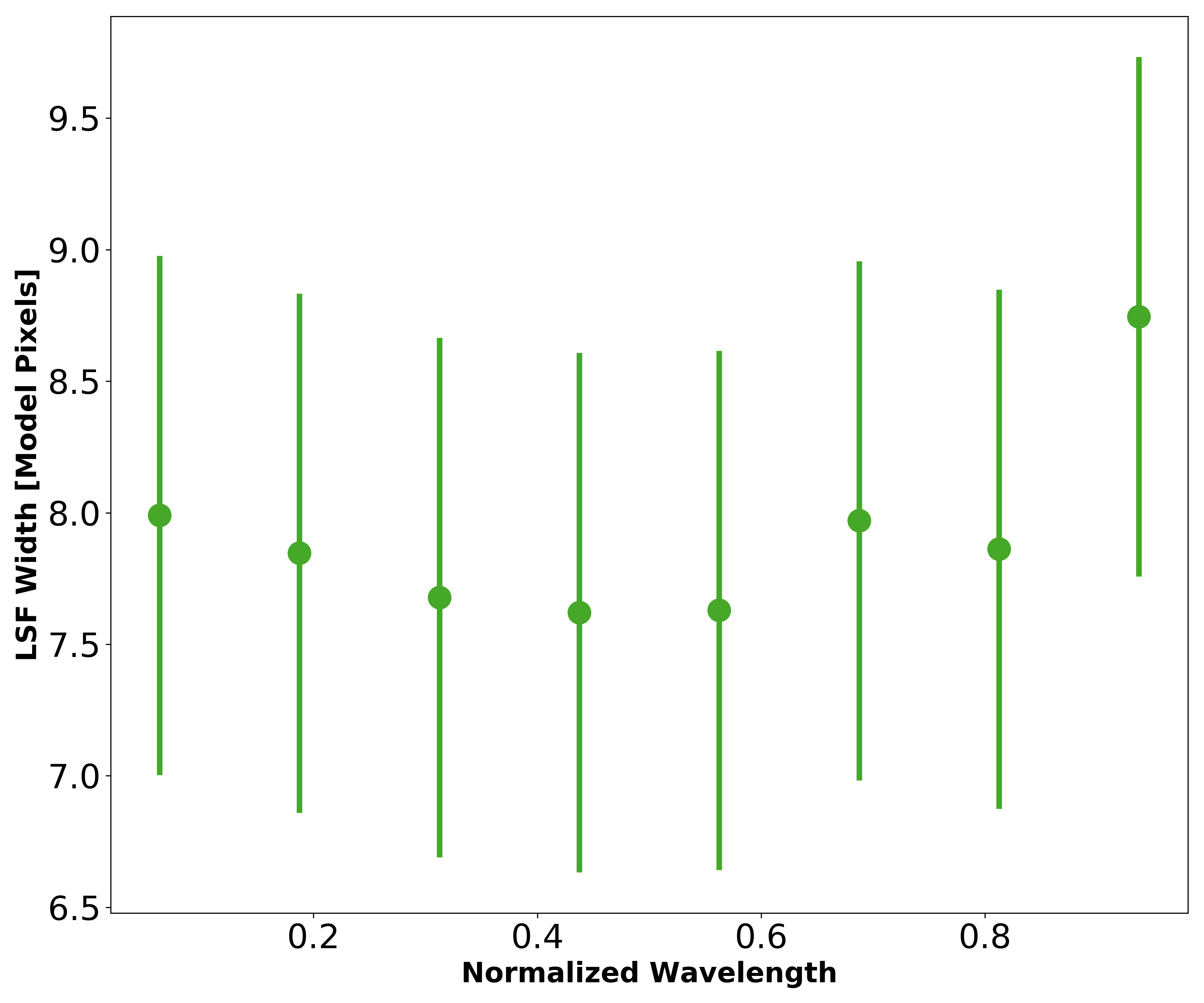
Like Gao et al. 2016 with CSHELL, we assess different parameterizations of our LSF model. With iSHELL’s larger spectral grasp, we find that a varying LSF model within the order can improve the RMS in fitting. If the LSF truly is dynamic across a single-order, then it would be advantageous to allow for a unique LSF model at each model pixel using spline continuity relations, similar to the wavelength solution and blaze function. Unfortunately this would be too computationally expensive having to compute over 16,000 LSF’s for a single model. Further, there is no reason to use a finer LSF model than a single resolution element (~0.03 nm, or 3 detector pixels). The downside of a binned LSF is it drastically increases the number of model parameters and therefore runtime. Further, from the limited number of cases performed with a dynamic LSF, we find that this degrades RV precision. A 3 Hermite term model with 8 equally sized bins across the detector (Fig. 31) typically yields ~5 ms-1 higher single-order RV precision, while a 7 Hermite term model (8 bins) is anywhere from 0–10 ms-1 worse on average. Since it is possible to over-fit the data, a lower RMS from a more complex LSF model does not necessarily lead to the lowest RV precision.
VIII.3 Other NIR Precise RV Instruments & Methodologies
We compare our results with other on-sky NIR precise RV spectrographs. Early instruments like NIRSPEC (McLean et al. 1995) on Keck were capable of 40–50 ms-1 precisions using tellurics as a wavelength reference and were mostly limited by the smaller spectral resolution of R~25,000 (Tanner et al. 2012). The CRIRES (Kaeufl et al. 2004) spectrograph on the VLT obtained 5 ms-1 long-term RVs at K-band using an ammonia gas cell for wavelength calibration, and was primarily limited by imperfect modeling of telluric lines (Bean et al. 2010). The Habitable Zone Planet Finder (HPF) spectrograph (Y- & J-band) on the 10 meter Hobby-Eberly telescope has reached 3 ms-1 long-term precisions on Barnard’s Star (Metcalf et al. 2019b). Unlike iSHELL which uses a gas cell to serve as a common optical path wavelength reference, HPF uses a laser frequency comb providing a series of evenly spaced emission lines to serve as a wavelength reference (Metcalf et al. 2019a). The CARMENES instrument utilizes two spectrographs (visible and J-, Y-band) with the goal of characterizing stellar activity through analyzing the color (wavelength) dependence on RVs. The visible arm has shown 1–5 ms-1 is possible (Reiners et al. 2018), but the NIR is still impacted by the mitigation of tellurics using the CCF method and the lower than expected (from synthetic spectra) RV information content in the Y- and J-bands (Tal-Or et al. 2018).
While not used here, the wobble pipeline (Bedell et al. 2019) is a second data-driven technique to retrieve and has shown notable precision at optical wavelengths further validating our approach. In their work, an initial template is determined in the same method we outline above, but is then treated as a high resolution grid of values to be optimized. The grid must be the same for all spectra, but each is then Doppler shifted with a unique . This implies all spectra are optimized simultaneously with a single likelihood function, although the temporal variations are fit separately.
VIII.4 Prospects for iSHELL Planet Confirmation
With the launch of the NASA TESS (Transiting Exoplanet Survey Satellite) mission, there will be a plethora of planet candidates needing RV follow-up to constrain the mass, and therefore density of the planets. Given our demonstrated precision, many of these candidates orbiting K and M dwarfs brighter than and with velocity semi-amplitudes 3 ms-1 will be detectable with iSHELL. From the existing list of TESS objects of interest77 7 https://tess.mit.edu/toi-releases/ that meet this brightness and predicted semi-amplitude criteria, and the total estimated yield from Barclay et al. 2018, we estimate ~100 candidates will be amenable to follow-up with iSHELL. We have already demonstrated iSHELL’s planet detection capabilities with the discoveries of a Jovian planet system (Plavchan et al. 2019, submitted).
With its unique wavelength coverage, iSHELL measurements will provide a valuable window to confirm planets around K and M dwarfs, particularly those that are more magnetically active and less amenable to confirmation at visible wavelengths. To first order, we expect RV variations induced by stellar activity from stellar rotation modulated spots and plages to be reduced in amplitude in the NIR w/r/t to the visible by a factor proportional to the frequency ratio (Reiners et al. 2010). For example, a star with 5 ms-1 stellar activity in the visible may be reduced to 1.5 ms-1 in the NIR, improving sensitivity to planets with velocity semi-amplitudes of ~1–10 ms-1.
IX Summary & Future Improvements
We have developed a data analysis pipeline that can robustly extract RVs from K-Band spectra taken with the iSHELL spectrograph on the NASA IRTF using a gas cell as a wavelength reference. By iteratively minimizing the RMS between the model and observed spectrum, we retrieve both the best-fit RVs as well as a deconvolved high-resolution spectrum of the star. The model uses 48 parameters and accounts for our gas cell, tellurics, fringing, blaze, LSF, and wavelength solution. Our initial efforts have shown 5 ms-1 precision for Barnard’s Star and 61 Cyg A over a ~1 year baseline, and 3 ms-1 for GJ 15 A over one month. We note a summary of accomplishments shown in this work below.
- 1.
Achieve 5 ms-1 RV precision over 1 year with
- •
A unique calibration source at an unfrequented wavelength range for precise RV work,
- •
A spectrograph that slews with the telescope at Cassegrain focus,
- •
- 2.
In the presence of
- •
Deep and dynamic telluric lines across entire spectral orders,
- •
Non-standard fringing greatly sophisticating an already high-dimensional forward model,
- •
Starting from the assumption of an unknown stellar template.
- •
Future improvements to our analysis may come with a more sophisticated RV forward model. We have yet to utilize the large overlap of the echelle orders and order-to-order parameter consistency. Low SNR regions (from blaze modulation) near the ends of order are closer to the blaze wavelength (and thus a higher SNR) in orders which will help yield better estimates of the proper line shapes across the entire order, as well as bad pixel flagging. Lastly, we may want to introduce a time-varying telluric or stellar component to account for dynamic features (in a similar fashion to the wobble pipeline).
X Acknowledgments
We acknowledge support from the the National Science Foundation (Astronomy and Astrophysics grant 1716202) and George Mason University start-up funds. All RVs extracted through PySHELL were run on ARGO, a research computing cluster provided by the Office of Research Computing, and the exo computer cluster, both at George Mason University, VA. We thank John Rayner and the IRTF and iSHELL support astronomers, telescope operators, and engineers for the dedicated efforts in helping enable the collection of the data presented in this paper. We acknowledge Guillem Anglada-Escudé, Russel White, Todd Henry, and Bernie Walp for their feedback. The authors wish to recognize and acknowledge the very significant cultural role and reverence that the summit of Maunakea has always had within the indigenous Hawaiian community. We are most fortunate to have the opportunity to conduct observations from this mountain.
References
- Aigrain et al. (2017) Aigrain, S., Parviainen, H., Roberts, S., Reece, S., & Evans, T. 2017, MNRAS, 471, 759
- Allard et al. (2003) Allard, F., Guillot, T., Ludwig, H.-G., et al. 2003, in IAU Symposium, Vol. 211, Brown Dwarfs, ed. E. Martín, 325
- Allard et al. (2011) Allard, F., Homeier, D., & Freytag, B. 2011, in Astronomical Society of the Pacific Conference Series, Vol. 448, 16th Cambridge Workshop on Cool Stars, Stellar Systems, and the Sun, ed. C. Johns-Krull, M. K. Browning, & A. A. West, 91
- Andrae et al. (2010) Andrae, R., Schulze-Hartung, T., & Melchior, P. 2010, arXiv e-prints, arXiv:1012.3754
- Anglada-Escudé et al. (2012) Anglada-Escudé, G., Plavchan, P., Mills, S., et al. 2012, PASP, 124, 586
- Anglada-Escudé et al. (2013) Anglada-Escudé, G., Butler, R. P., Reiners, A., et al. 2013, Astronomische Nachrichten, 334, 184
- Anglada-Escudé et al. (2016) Anglada-Escudé, G., Amado, P. J., Barnes, J., et al. 2016, Nature, 536, 437
- Arfken G. (2012) Arfken G., Weber H., H. F. 2012, Mathematical Methods for Physicists (Academic press)
- Bailey et al. (2012) Bailey, III, J. I., White, R. J., Blake, C. H., et al. 2012, ApJ, 749, 16
- Bajzer & Penzar (1999) Bajzer, Z., & Penzar, I. 1999, simps
- Barclay et al. (2018) Barclay, T., Pepper, J., & Quintana, E. V. 2018, ApJS, 239, 2
- Basri et al. (2010) Basri, G., Walkowicz, L. M., Batalha, N., et al. 2010, ApJ, 713, L155
- Bean et al. (2010) Bean, J. L., Seifahrt, A., Hartman, H., et al. 2010, ApJ, 713, 410
- Bedell et al. (2019) Bedell, M., Hogg, D. W., Foreman-Mackey, D., Montet, B. T., & Luger, R. 2019, arXiv e-prints, arXiv:1901.00503
- Bertaux et al. (2014) Bertaux, J. L., Lallement, R., Ferron, S., Boonne, C., & Bodichon, R. 2014, A&A, 564, A46
- Blake et al. (2010) Blake, C. H., Charbonneau, D., & White, R. J. 2010, ApJ, 723, 684
- Bouchy et al. (2001) Bouchy, F., Pepe, F., & Queloz, D. 2001, A&A, 374, 733
- Butler et al. (1996) Butler, R. P., Marcy, G. W., Williams, E., et al. 1996, PASP, 108, 500
- Choi et al. (2012) Choi, J., Marcy, G., & Howard, A. 2012, in American Astronomical Society Meeting Abstracts, Vol. 219, American Astronomical Society Meeting Abstracts #219, 245.04
- Crockett et al. (2011) Crockett, C. J., Mahmud, N. I., Prato, L., et al. 2011, ApJ, 735, 78
- Crockett et al. (2012) —. 2012, ApJ, 761, 164
- Fischer et al. (2016) Fischer, D. A., Anglada-Escude, G., Arriagada, P., et al. 2016, PASP, 128, 066001
- Gao et al. (2016) Gao, P., Plavchan, P., Gagné, J., et al. 2016, PASP, 128, 104501
- Gopalan et al. (2016) Gopalan, G., Plavchan, P., van Eyken, J., et al. 2016, PASP, 128, 084504
- Horne (1986) Horne, K. 1986, PASP, 98, 609
- Howard et al. (2014) Howard, A. W., Marcy, G. W., Fischer, D. A., et al. 2014, ApJ, 794, 51
- Hunter (2007) Hunter, J. D. 2007, Computing in Science & Engineering, 9, 90
- Jenkins et al. (2009) Jenkins, J. S., Ramsey, L. W., Jones, H. R. A., et al. 2009, ApJ, 704, 975
- Jones et al. (2001) Jones, E., Oliphant, T., Peterson, P., et al. 2001, SciPy: Open source scientific tools for Python
- Kaeufl et al. (2004) Kaeufl, H.-U., Ballester, P., Biereichel, P., et al. 2004, in Proc. SPIE, Vol. 5492, Ground-based Instrumentation for Astronomy, ed. A. F. M. Moorwood & M. Iye, 1218–1227
- Kovács et al. (2005) Kovács, G., Bakos, G., & Noyes, R. W. 2005, MNRAS, 356, 557
- Lipson S.G. (1995) Lipson S.G., Lipson H., T. D. 1995, Optical Physics (Cambridge)
- Mahmud et al. (2011) Mahmud, N. I., Crockett, C. J., Johns-Krull, C. M., et al. 2011, ApJ, 736, 123
- Marchwinski et al. (2015) Marchwinski, R. C., Mahadevan, S., Robertson, P., Ramsey, L., & Harder, J. 2015, ApJ, 798, 63
- Martín et al. (2010) Martín, E. L., Guenther, E., Del Burgo, C., et al. 2010, in Astronomical Society of the Pacific Conference Series, Vol. 430, Pathways Towards Habitable Planets, ed. V. Coudé du Foresto, D. M. Gelino, & I. Ribas, 181
- Mayor & Queloz (1995) Mayor, M., & Queloz, D. 1995, Nature, 378, 355
- McLean et al. (1995) McLean, I. S., Becklin, E. E., Figer, D. F., et al. 1995, in Proc. SPIE, Vol. 2475, Infrared Detectors and Instrumentation for Astronomy, ed. A. M. Fowler, 350–358
- Metcalf et al. (2019a) Metcalf, A. J., Fredrick, C. D., Terrien, R. C., Papp, S. B., & Diddams, S. A. 2019a, arXiv e-prints, arXiv:1902.02817
- Metcalf et al. (2019b) Metcalf, A. J., Anderson, T., Bender, C. F., et al. 2019b, arXiv e-prints, arXiv:1902.00500
- Newton et al. (2016) Newton, E. R., Irwin, J., Charbonneau, D., Berta-Thompson, Z. K., & Dittmann, J. A. 2016, ApJ, 821, L19
- Pearson (1895) Pearson, K. 1895, Proceedings of the Royal Society of London Series I, 58, 240
- Plavchan et al. (2015) Plavchan, P., Latham, D., Gaudi, S., et al. 2015, arXiv e-prints, arXiv:1503.01770
- Plavchan et al. (2013) Plavchan, P. P., Anglada-Escude, G., White, R., et al. 2013, in Proc. SPIE, Vol. 8864, Techniques and Instrumentation for Detection of Exoplanets VI, 88641J
- Rayner et al. (2016) Rayner, J., Tokunaga, A., Jaffe, D., et al. 2016, in Proc. SPIE, Vol. 9908, Ground-based and Airborne Instrumentation for Astronomy VI, 990884
- RECONS (2018) RECONS. 2018, RECONS Research Consortium on Nearby Stars
- Reiners et al. (2010) Reiners, A., Bean, J. L., Huber, K. F., et al. 2010, ApJ, 710, 432
- Reiners et al. (2018) Reiners, A., Zechmeister, M., Caballero, J. A., et al. 2018, A&A, 612, A49
- Ribas et al. (2018) Ribas, I., Tuomi, M., Reiners, A., et al. 2018, Nature, 563, 365
- Robertson et al. (2015) Robertson, P., Roy, A., & Mahadevan, S. 2015, ApJ, 805, L22
- Sameshima et al. (2018) Sameshima, H., Matsunaga, N., Kobayashi, N., et al. 2018, PASP, 130, 074502
- Sato et al. (2002) Sato, B., Kambe, E., Takeda, Y., Izumiura, H., & Ando, H. 2002, PASJ, 54, 873
- Seifahrt et al. (2010) Seifahrt, A., Käufl, H. U., Zängl, G., et al. 2010, A&A, 524, A11
- Still & Barclay (2012) Still, M., & Barclay, T. 2012, PyKE: Reduction and analysis of Kepler Simple Aperture Photometry data, Astrophysics Source Code Library, ascl:1208.004
- Tal-Or et al. (2018) Tal-Or, L., Zechmeister, M., Reiners, A., et al. 2018, A&A, 614, A122
- Tanner et al. (2012) Tanner, A., White, R., Bailey, J., et al. 2012, ApJS, 203, 10
- Tronsgaard et al. (2019) Tronsgaard, R., Bucchave, L., Wright, J., Eastman, J., & Blackman, R. 2019, MNRAS
- van Belle & von Braun (2009) van Belle, G. T., & von Braun, K. 2009, ApJ, 694, 1085
- Vanderburg et al. (2016) Vanderburg, A., Plavchan, P., Johnson, J. A., et al. 2016, MNRAS, 459, 3565
- West et al. (2004) West, A. A., Hawley, S. L., Walkowicz, L. M., et al. 2004, AJ, 128, 426
- Wright & Eastman (2014) Wright, J. T., & Eastman, J. D. 2014, PASP, 126, 838