The intrinsic reddening of the Magellanic Clouds as traced by background galaxies – I. The bar and outskirts of the Small Magellanic CloudThe intrinsic reddening of the Magellanic Clouds as traced by background galaxies – I. The bar and outskirts of the Small Magellanic Cloud–2019
Abstract
We present a method to map the total intrinsic reddening of a foreground extinguishing medium via the analysis of spectral energy distributions (SEDs) of background galaxies. In this pilot study, we implement this technique in two distinct regions of the Small Magellanic Cloud (SMC) – the bar and the southern outskirts – using a combination of optical and near-infrared broadband imaging. We adopt the lephare -minimisation SED-fitting routine and various samples of galaxies and/or quasi-stellar objects to investigate the intrinsic reddening. We find that only when we construct reddening maps using objects classified as galaxies with low levels of intrinsic reddening (i.e. ellipticals/lenticulars and early-type spirals), the resultant maps are consistent with previous literature determinations i.e. the intrinsic reddening of the SMC bar is higher than that in the outer environs. We employ two sets of galaxy templates – one theoretical and one empirical – to test for template dependencies in the resulting reddening maps and find that the theoretical templates imply systematically higher reddening values by up to 0.20 mag in . A comparison with previous reddening maps, based on the stellar components of the SMC, typically shows reasonable agreement. There is, however, significant variation amongst the literature reddening maps as to the level of intrinsic reddening associated with the bar. Thus, it is difficult to unambiguously state that instances of significant discrepancies are the result of appreciable levels of dust not accounted for in some literature reddening maps or whether they reflect issues with our adopted methodology.
Keywords:
(galaxies:) Magellanic Clouds – galaxies: photometry – galaxies: ISM – surveys – (ISM:) dust, extinction1 Introduction
The Large and Small Magellanic Clouds (LMC and SMC) are the largest, most massive dwarf satellite galaxies of the Milky Way (MW), and represent an unparallelled testbed to study the formation and evolution of galaxies. Given the interactions between the LMC and SMC as well as the Magellanic Clouds (MCs) and the MW (see e.g Olsen et al. 2011; Besla et al. 2012; Diaz & Bekki 2012; Choi et al. 2018), they provide a unique insight into the effects of such interactions on the structure and history of the galaxies. In a cosmological context, interacting galaxies can also be used to study the effects of minor merger events, which are believed to be important for the formation of MW-like galaxy haloes (Brook et al. 2004; Read et al. 2008).
Studying interacting galaxies, however, is non-trivial as the underlying structure and stellar populations have both been shaped by prior events. A dominant factor contributing to the uncertainties is the internal dust of the galaxy, which is generally non-uniform and can thus have a significant effect on the derived physical properties. The reddening is typically inferred through colour-magnitude diagram (CMD) analyses.
The reddening of the MCs has been extensively investigated, based predominantly on various stellar components of the MCs. Such methods include comparing the colour of the red clump and/or RR Lyrae stars with the unreddened colour predicted by stellar evolutionary models at the corresponding metallicity (see e.g. Udalski et al. 1999a; Udalski et al. 1999b; Subramanian & Subramaniam 2009; Subramanian & Subramaniam 2012; Haschke et al. 2011; Tatton et al. 2013; Choi et al. 2018), multi-band fitting of the reddening law to the apparent distance moduli of Cepheids to derive individual reddening values (see e.g. Inno et al. 2016), as well as comparing multi-band photometry with stellar atmospheric models (see e.g. Zaritsky et al. 2002; Zaritsky et al. 2004). In addition, longer-wavelength mid-/far-infrared (IR), microwave and radio observations of the MCs have also played crucial roles in not only mapping, but also quantifying the dust content of the MCs (see e.g. Gordon et al. 2003; Leroy et al. 2007; Bernard et al. 2008; Israel et al. 2010).
Here we present a pilot study to map and quantify the total intrinsic reddening of the MCs based on observations of background galaxies behind the MCs. Whilst background galaxies have been used in the past to probe the reddening of the MCs (see e.g. Hodge 1969; Gurwell & Hodge 1990; van Loon et al. 1997; Dutra et al. 2001; Krienke & Hodge 2001), these studies have typically used only a small number of galaxies to place constraints on the reddening along given line of sights based on either their observed colours or through spectroscopic analysis. In this study, we combine optical and near-IR photometric data to construct eight-band spectral energy distributions (SEDs) which we use to map the reddening across the MCs as well as determine the total line-of-sight reddening. This technique has the advantage that it does not rely on the use of stars in the CMD i.e. it is independent of the tool used to study the underlying stellar populations. Furthermore, as it does not involve the use of variable stars, the technique is not spatially limited to those which have been catalogued through time-series photometric identification of light curves.
The structure of the paper is as follows. In Section 2 we introduce the photometric data sets, describe our galaxy selection procedure and also discuss the photometric pipeline used to create the SEDs. Section 3 describes the fitting of the galaxy SEDs and in Section 4 we introduce the method adopted to determine the intrinsic reddening. We discuss our results in Section 5 and in Section 6 we present our conclusions.
2 Photometric data set
Our data set consists of optical and near-IR photometry taken as part of the Survey of the MAgellanic Stellar History (SMASH; Nidever et al. 2017) and the Visible and Infrared Survey Telescope for Astronomy (VISTA) survey of the Magellanic Clouds system (VMC; Cioni et al. 2011), which together are composed of eight bandpasses () covering the wavelength range 0.3–2.5 m.
2.1 SMASH optical data
SMASH is a National Optical Astronomy Observatory (NOAO) community Dark Energy Camera (DECam) survey of the MC system which maps 480 deg2 (distributed across an area of 2400 deg2 at a 20 per cent filling factor) with limiting (AB) magnitudes of 24 mag in . DECam (Flaugher et al. 2015) mounted on the Blanco 4-m telescope at Cerro Tololo Inter-American Observatory (CTIO) comprises 62 CCDs (of which were functional throughout the majority of the SMASH observations; see Nidever et al. 2017 for details) covering a field of view of 3 deg2 with a pixel scale of 0.27′′. All scheduled SMASH observations have now been completed from which we determine a median image seeing of 1.21, 1.12, 1.00, 0.94 and 0.89 arcsec in , respectively, with a standard deviation ranging from 0.32 () to 0.24 arcsec (). To cover the gaps between the CCDs, the survey’s observing strategy consists of deep exposures (999 s in and 801 s in ), in addition to three sets of short 60 s exposures in with large, half-CCD offsets between each set.
2.2 VMC near-IR data
The VMC is one of the first six public surveys commissioned by the European Southern Observatory (ESO) and covers 170 deg2 of the MC system with limiting (AB) magnitudes of 22 mag in . The VISTA IR CAMera (VIRCAM; Sutherland et al. 2015) comprises 16 detectors arranged in a sparse-filled 4 4 rectangular grid within the 1.65 degree diameter field of view, with a pixel scale of 0.34′′, and provides an active field of 0.60 deg2 on pixels (known as a pawprint). Due to gaps of 0.9 detector width in the -direction and 0.425 detector width in the -direction a set of six offset pawprints are observed to give one filled rectangular area consisting of a central rectangle of 1.475 1.017 degrees covered by at least two of the six pawprints (1.5 deg2); plus two thin stripes each 0.092 degrees wide (along the two long edges) covered by just one pawprint, giving a total contiguously covered area of 1.77 deg2 (known as a tile). VMC observations were completed in October 2018 and from these we determine a median image seeing of 1.03, 1.00 and 0.93 arcsec in with standard deviations of 0.13, 0.10 and 0.08 arcsec, respectively. The VMC is a multi-epoch survey providing three epochs in and 12 in , so accounting for the individual pawprint exposures, the number of offset exposures and the number of epochs in each band, the total exposure times per tile are 2400 s in and 9000 s in . Repeat observations within each survey suggest a photometric precision of better than 2 per cent in all bands.

This pilot study represents a proof of concept for our technique to determine the total intrinsic reddening using galaxies observed through the MCs and as such we focus on only two VMC tiles. The complete analysis of the combined SMASH-VMC footprint is still underway. In this paper we focus on tiles SMC 2_4 and SMC 4_3 from the VMC survey – hereafter referred to as the outskirts and bar regions of the SMC – centred at and , respectively. Fig. 1 shows the positions of these tiles overlaid on a stellar density plot of the central region of the SMC for which we have adopted the centre of the SMC () as provided by the HYPERLEDA catalogue of Paturel et al. 2003. This figure demonstrates that the two tiles probe regions of different stellar density of the SMC, and sample large enough areas to encompass different levels of intrinsic reddening.
2.3 A priori identification of background galaxies
To identify background galaxies we adopt a combination of colour-magnitude and morphological selections. Given the relatively crowded nature of the MCs and the cleaner separation between stars and galaxies in near-IR CMDs (see e.g. Maddox et al. 2012; Cioni et al. 2014), compared to their optical counterparts (see e.g. Nidever et al. 2019), we opt to identify background galaxies using the VMC PSF photometric catalogues. These catalogues are generated from homogenised deep tiles which are created by combining pawprints from different epochs (see Rubele et al. 2015), which “smears” any variability. Pawprints which were taken in sub-optimal observing conditions (e.g. high seeing, patchy cloud cover, etc.) were not included in the creation of the deep tiles.
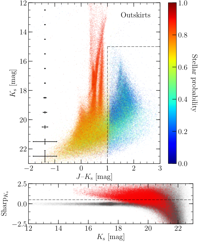
We initially define our sample of galaxies as those objects which satisfy both – mag and mag in the , – CMD, thereby ensuring that our objects are detected in at least two bands. We impose the bright magnitude cut to avoid including intrinsically reddened evolved stars and/or young stellar objects in our sample. The top panel of Fig. 2 shows our initial colour-magnitude selection for the outskirts region of the SMC. This sample is further refined using a combination of the stellar probability and -band sharpness index11 1 The daophot sharpness index is proportional to the ratio of the FWHM of the object to the FWHM of the PSF model and so extended objects will tend to have values appreciably larger than zero. provided for each unique object as part of the VMC PSF catalogues. Stellar probabilities are calculated based on a combination of the position in the colour-colour diagram, the local completeness level (as determined by artificial star tests; see Rubele et al. 2011) and the daophot (Stetson 1987) sharpness index. Fig. 2 clearly shows that the objects initially identified through our colour-magnitude selection have low stellar probabilities (mean value of 0.33) and also exhibit significantly larger sharpness indices than one would expect for stellar objects. We adopt the sharpness index as measured from the -band images as the VMC observing requirements ensure the highest quality seeing in this bandpass (see Cioni et al. 2011). We therefore include the criteria that objects which satisfy our initial colour-magnitude selection must also have stellar probabilities of less than 0.33 and -band sharpness indices of greater than 0.5. These combined criteria result in the identification of 29,843 and 18,509 potential galaxies in the outskirts and bar regions of the SMC, respectively.
There will of course be a number of sources with stellar probabilities of less than 0.33 at bluer colours. The available colour-magnitude and morphological information is insufficient to differentiate between whether such objects are actually galaxies or simply blended stars, and so to retain a relatively clean sample of galaxies we do not loosen the aforementioned criteria. The objects which meet these selection criteria, however, will invariably include a number of both quasi-stellar objects (QSOs) and stars (especially at fainter magnitudes where the -band sharpness index distribution begins to bloom; see the bottom panel of Fig. 2). Of these, stars are genuine contaminants as they are not observed through the MCs and hence their SEDs do not include the imprints of the intrinsic MC reddening. QSOs, on the other hand, can be used in exactly the same way as the background galaxies. Further details pertaining to how we differentiate between different types of objects (galaxies, QSOs and stars) are presented in Section 3 in which we describe our adopted SED-fitting code.
2.4 lambdar photometry
Fluxes for each of our targets are measured using the Lambda Adaptive Multi-Band Deblending Algorithm in R (lambdar, v0.20; Wright et al. 2016). lambdar is designed to perform accurate matched aperture photometry, of pre-defined sources, across images that are neither pixel nor PSF matched. To perform the photometry lambdar requires two inputs; a catalogue of objects containing positions and aperture parameters as well as a FITS image with World Coordinate System (WCS) astrometry. We also took advantage of the lambdar functionality to mask out contaminants to remove the contribution of sources within 3 arcsec of each object.
As a result of crowding, we use lambdar to not only measure fluxes using standard (circular) apertures of diameter 3 arcsec [see e.g. the Cosmic Evolution Survey (COSMOS; Scoville et al. 2007) optical and near-IR photometric catalogue produced by Capak et al. 2007], but also PSF-weighted apertures which will result in more reliable deblending of sources. PSF-weighted apertures preferentially extract information from the central regions of galaxies which acts to both reduce the noise on the estimates caused by noisy low-flux pixels in the galaxy’s outskirts and reduce the complexity of the SED required to model the galaxy by probing the (typically redder) central regions of the galaxy. By using fluxes extracted using PSF-weighted apertures, however, one implicitly ignores the self-contamination of the inner-galaxy profile by flux from the outskirts of the galaxy. If the PSF between different bands varies significantly, this could result in slightly incorrect flux estimates and/or systematics, however as the size of the PSFs across all eight bands are similar (see Sections 2.1 and 2.2), this essentially means that the contamination is consistent in each band and thus should not significantly affect the resultant SED. Fig. 3 shows postage stamp cut-outs of typical and 20 mag galaxies in the outskirts region of the SMC in each of the eight bandpasses with a 3 arcsec diameter aperture overlaid.

Specific details of lambdar are presented by Wright et al. 2016, although there have been some developments to the code since its publication which are relevant to the work presented here. In particular, the program now includes the functionality to estimate the PSF of an input image by stacking suitably segregated high-signal-to-noise point sources. As the imaging under analysis here can be significantly affected by crowding, this functionality is able to return high fidelity PSFs and thus is particularly useful. To ensure that our final PSF estimate is robust, we have generated PSFs for a given image using different samples of point sources. The PSF estimates are seen to vary by less than half a percent in integrated area, suggesting that the choice of which point sources contribute to the stacked PSF is not critical to the fidelity of the PSF estimate. Other than the new PSF estimation, the code remains largely unchanged since v0.12 described by Wright et al. 2016. Nonetheless, some minor changes and genuine bug fixes have been implemented, and are all documented in the GitHub repository commit history22 2 https://github.com/AngusWright/LAMBDAR.
For our input FITS images we downloaded the VMC images covering the bar and outskirts regions of the SMC from the VISTA Science Archive33 3 http://horus.roe.ac.uk/vsa. VMC data for the bar region of the SMC (SMC 4_3) are publicly available and those for the outskirts (SMC 2_4) will soon be released as part of VMC Data Release 5 which is in preparation. (VSA; Cross et al. 2012). We adopt the deep stacks (the stacked pawprints from different epochs, each of which comprises 16 detectors) as opposed to the single deep tiles as the latter can suffer from significant jumps in the sky background level on small scales due to the process of combining different pawprints in the creation of the tile44 4 Despite known issues with some of the VIRCAM detectors (see http://casu.ast.cam.ac.uk/surveys-projects/vista/technical/known-issues for a full description), we do not notice any obvious trends in the reddening maps which would suggest that these significantly affect our results.. To calibrate the near-IR data onto an AB magnitude system, we follow the prescription of González-Fernández et al. 2018.
To calibrate the optical data onto a native DECam AB magnitude system we remove the SMASH colour terms introduced to calibrate the photometry onto a quasi-SDSS system. This process was performed on a CCD-by-CCD basis and involves the use of “fiducial” colours (as defined by the SDSS standard stars and which includes the band one wishes to calibrate; see Nidever et al. 2017). For our “fiducial” colours we adopt the following values: –, –, –, –, – mag for the -, -, -, - and -bands, respectively. The uncertainties on the coefficients used in the SMASH transformation equations are very small (less than 1 per cent) and as we perform a transformation with a fixed fiducial colour the resultant uncertainties on the DECam AB magnitude photometry should be equally small.
| Region | Sample | No. of objects |
|---|---|---|
| Outskirts | Aper. | 29,606 (91.4, 6.1, 1.5, 0.5, 0.5) |
| PSF | 29,788 (93.9, 4.7, 0.9, 0.3, 0.2) | |
| Bar | Aper. | 16,796 (66.3, 18.9, 8.0, 4.2, 2.6) |
| PSF | 18,248 (74.2, 15.9, 6.2, 2.6, 1.1) |
Given the observing strategy of both the SMASH and VMC surveys, each galaxy in our sample is observed multiple times except for objects in two narrow strips along the length of the VIRCAM array (see fig. 3 of Cross et al. 2012). Although these regions, except for the lower strip of the outskirts region of the SMC which corresponds to the lower limit of the VMC coverage, are covered by observations of other tiles in the VMC survey, we do not include these additional measurements. The final flux for each object is simply the weighted mean of all available measurements in that band and for which we set the weights equal to the inverse square of the corresponding uncertainty on the flux. To ensure reliable SED fits, we only retain objects for which we measure positive fluxes in at least four out of the eight available bandpasses. Given that we have extracted fluxes using both standard (circular) as well as PSF-weighted apertures, the number of resultant objects for a given tile in both cases is not necessarily the same. Our final standard aperture and PSF-weighted aperture photometric catalogues have a total of 29,606 and 29,788 objects, respectively, for the outskirts region of the SMC, whereas for the bar region the catalogues contain 16,796 and 18,248 objects (see Table 1).
2.5 Accounting for foreground Milky Way reddening
The final step in the creation of our galaxy SEDs is to account for diffuse foreground MW reddening. The line-of-sight reddening towards a given galaxy includes several components, and thus by removing the MW component this will make it easier to infer the intrinsic reddening of the two SMC tiles from the SEDs. We determine the corresponding value for a given position using the Python module sfdmap55 5 https://github.com/kbarbary/sfdmap which linearly interpolates within the Schlegel et al. 1998 dust maps. Following Schlafly & Finkbeiner 2011, a scaling of 0.86 is applied as standard to the SFD98 values to reflect the fact that these values were calculated using the Cardelli et al. 1989 and O’Donnell 1994 extinction laws, which have since been shown to overestimate the resultant reddening values (see also Schlafly et al. 2010; Yuan et al. 2013). To convert a given value to extinction in a specific bandpass, we adopt the following coefficients:
| (1) |
The coefficients are taken from the Dark Energy Survey (DES) Data Release (DR) 1 paper by Abbott et al. 2018, whereas the coefficients are from González-Fernández et al. 201866 6 As the DES does not include -band observations the corresponding coefficient is not given by Abbott et al. 2018. This was instead calculated in exactly the same way as for the coefficients and kindly provided upon request by the DES collaboration.. These coefficients have been calculated assuming as well as account for the Schlafly & Finkbeiner 2011 recalibration, and should therefore be used in conjunction with the unscaled SFD98 values provided by sfdmap.

Fig. 4 shows the SFD98 foreground MW and residual intrinsic SMC reddening in the direction of the SMC. From the top panel of Fig. 4 it is clear that towards the Bar and Wing regions of the SMC the prescription adopted by SFD98 to convert the dust measurements into a foreground reddening becomes unreliable due to contamination from SMC sources (or unresolved temperature structure; see Appendix C of SFD98) leading to foreground values of almost 1.5 mag in places. Whilst the top panel of Fig. 4 appears to suggest that in the outer environs of the SMC the MW foreground reddening is essentially uniform, the bottom panel of Fig. 4 shows significant amounts of low-level variation in the SFD98 values. Regions in the north and west of the panel have systematically lower reddening values than regions in the south and east. Whether these variations are indeed genuine variations in the foreground MW reddening or are instead variations in the intrinsic SMC reddening is unclear.
In an attempt to account for the foreground MW reddening in a reasonable and systematic way, we estimate the median foreground reddening in the direction of the SMC by defining an annulus of width 0.2∘ at a radius of 2.5∘ from our adopted SMC centre (see Fig. 4). Using the VMC PSF catalogues, we extract all sources which lie within this annulus ( 1.9 objects) and use sfdmap to determine the corresponding SFD98 reddening values, from which we determine a median reddening and standard deviation of mag and 0.011 mag, respectively. Finally, we then apply this median value to all objects in our photometric catalogues and correspondingly de-redden the individual fluxes using the coefficients noted in Eqn. 1.
3 Fitting the SEDs of galaxies
Whilst there are many available sophisticated codes for modelling and interpreting galaxy SEDs (see http://www.sedfitting.org/ for a compilation of these), we adopt the lephare code77 7 http://cesam.lam.fr/lephare/lephare (developed by S. Arnouts and O. Ilbert). Our choice of SED-fitting code is primarily motivated by our goal to produce reddening maps of the MCs, but is also influenced by several additional factors. For instance, in addition to the MC reddening, it would be beneficial to have statistics related to the background galaxies, such as redshift and galaxy type, which could then be compared to other studies. Furthermore, given that our photometric catalogues still include some stellar contaminants which we would like to remove, the SED-fitting code needs to be flexible enough to allow us to fit not only galaxy templates, but also different sets of templates to the SEDs and determine which provides a better fit to the data. lephare is a minimisation template-fitting routine which allows us to fit distinct sets of templates (including QSOs and stars) and thus easily determine the best-fitting model for a given SED88 8 In practice it can be hard to reliably differentiate between galaxies and QSOs based only on the value of the fit as this can classify a significant number of normal galaxies as QSOs (O. Ilbert priv. comm.). Thus whilst in some studies only galaxy and stellar templates are considered (see e.g. Ilbert et al. 2006; Ilbert et al. 2009), we chose to include QSO templates as these may provide a better fit to the SED than those in our galaxy template sets. We therefore note that the numbers of classified galaxies and QSOs listed in the text should be treated with caution.. Importantly, lephare permits inclusion of the intrinsic reddening of background galaxies [expressed in terms of ] to vary as a free parameter and explicitly accounts for intergalactic reddening following the prescription of Madau 1995 in which a detailed model of the H I opacity of the Universe is constructed by analysing the effects of various absorption mechanisms on the broadband colours of cosmologically distant galaxies.
3.1 SED template libraries
To investigate to what extent the derived reddening values are template-dependent, we adopt two distinct sets of galaxy templates; one theoretical and the other empirical. Our base set of theoretical spectra (see Ilbert et al. 2009) comprises the three elliptical and six spiral (S0, Sa, Sb, Sc, Sd, Sdm) SEDs generated by Polletta et al. 2007 using the grasil code (Silva et al. 1998). Ilbert et al. 2009 found that these templates were unable to fully reproduce the bluest colours of the COSMOS sample of galaxies (Lilly et al. 2007) and so included an additional 12 starburst templates generated from the Bruzual & Charlot 2003 models ranging in time of the most recent starburst from 0.03–3 Gyr. Finally, Ilbert et al. 2009 linearly interpolated some of the Polletta et al. 2007 templates, so our final set of theoretical templates consists of 31 galaxy SEDs; seven elliptical, 12 spiral and 12 starburst. Our base set of empirical templates comprises six spectra including the four observed spectral types (Ell, Sbc, Scd, Irr) from Coleman et al. 1980 in addition to two starburst galaxies from Kinney et al. 1996. These templates were first extrapolated beyond 1 m using the gissel synthetic models of Bruzual & Charlot 2003 and then optimised using the rest-frame fluxes of galaxies with spectroscopic redshift determinations in the VIMOS VLT Deep Survey (VVDS; see Ilbert et al. 2006 for details). Finally, to refine the sampling in colour- space, pairs of templates were linearly interpolated to create a final set of 62 SEDs. The sets of 31 theoretical and 62 empirical templates are referred to as COSMOS and AVEROI_NEW in lephare and shall henceforth be referred to as such.
In addition to our galaxy templates, we also adopt two further sets of templates corresponding to QSOs and stars. The QSO templates consist of 10 SEDs taken from the study of Polletta et al. 2007 which includes spectra of moderately luminous active galactic nuclei (AGN) representing Seyfert 1.8 and Seyfert 2 galaxies, optically selected QSOs with different values of IR/optical flux ratios, type 2 QSOs as well as composite AGN+starburst galaxies (see Polletta et al. 2007 for details). The stellar templates comprise a total of 235 spectra including the 131 spectra encompassing all normal spectral types and luminosity classes at solar abundance as well as metal-rich and metal-poor F–K dwarfs and G–K giants from Pickles 1998, 100 theoretical spectra of late-type dwarfs of different effective temperatures and surface gravities from Chabrier et al. 2000, and four white dwarf spectra from Bohlin et al. 1995. Although the stellar templates do not include inherently dusty objects such as Carbon and asymptotic giant branch stars, our criteria to select potential galaxies (see Section 2.3) should ensure that these are not an issue.
To compute the fluxes for our templates in the combined DECam and VIRCAM bandpasses, all templates were convolved with the corresponding system responses which are available at the NOAO and ESO webpages, respectively99 9 The DECam responses are available at http://www.ctio.noao.edu/noao/content/DECam-filter-information, whereas the VIRCAM responses are available at http://www.eso.org/sci/facilities/paranal/instruments/vircam/inst.html. Note that as the absolute calibration/normalisation of the DES DR1 bandpasses is not yet available on the DECam webpages, we have instead adopted the older system responses which are still provided for legacy use.. Emission line fluxes can have a significant effect on the magnitudes and colours of galaxies as a function of redshift, especially if there is significant ongoing star formation (see e.g. Jouvel et al. 2009). lephare allows such fluxes to be included in the theoretical magnitudes derived from the galaxy templates and so in order to better reproduce the colours of such galaxies we choose to include these (see Ilbert et al. 2009 for details regarding the implementation).
3.2 Redshift prior
Although the combination of optical and near-IR bands significantly reduces the intrinsic scatter of derived photometric redshifts as well as the rate of catastrophic failures (see e.g. Le Fèvre et al. 2013; Wright et al. 2018), the colours of the adopted templates can be degenerate with redshift. To minimise spurious likelihood peaks in the redshift distribution, we include a Bayesian redshift prior which describes the redshift probability distribution for galaxies as a function of spectral type (see e.g. Benítez 2000; Ilbert et al. 2006) and which has been calibrated using the robust VVDS spectroscopic sample (Le Fèvre et al. 2005).
3.3 Extinction law
Ilbert et al. 2009 used the COSMOS galaxy sample (Lilly et al. 2007) to test different extinction laws to determine the best extinction law to adopt for a given spectral type. Their analysis demonstrated that the extinction law as measured for the SMC by Prevot et al. 1984 is well suited for ellipticals, spirals and a subset of starburst galaxies, whereas for bluer starburst galaxies the Calzetti et al. 2000 extinction law as determined from observations of starburst galaxies is more appropriate. The extinction law for the two starburst galaxies included in the original six spectra from which the AVEROI_NEW template set was created is best described by the Prevot et al. 1984 formalism and thus we adopt this law for the AVEROI_NEW templates. For the COSMOS templates, however, we follow the prescription described by Ilbert et al. 2009 regarding which extinction law to use for a particular galaxy template. For our QSO templates we also adopt the Prevot et al. 1984 extinction law as this has been found to reproduce the dust reddening of most QSOs at both high and low redshifts (see e.g. Gallerani et al. 2010). To limit degeneracies in the best-fitting solutions (see e.g. Arnouts et al. 2007), we allow the reddening to vary for the galaxy and QSO templates from to 0.5 mag in steps of mag.
It is worth stressing that all adopted galaxy and QSO templates already include a certain level of dust extinction, either due to a formulated prescription in the code used to create the SEDs or due to the fact that they are empirical templates. So, even if highly obscured objects are present in our sample, a combination of the template including some extinction and the possibility to include additional extinction should ensure such objects are well fitted.
3.4 Systematic offsets
Potential uncertainties in both the absolute calibration of the photometric zero points as well as the predicted fluxes of the template SEDs, resulting from the adopted bandpass response functions and/or an incomplete template set, can result in zero point offsets between the predicted and observed colours (see e.g. Ilbert et al. 2006). The standard approach to account for such uncertainties is to use a large representative sample of galaxies with spectroscopic redshifts (i.e. covering the same part of the sky and with photometry using the same instrumental set-up) and iteratively calculate the required correction factor to ensure that the difference between the predicted and observed magnitudes at a given redshift is less than a few mmag (see e.g. Capak et al. 2004; Ilbert et al. 2009). Unfortunately, such a representative sample of galaxies behind the SMC does not exist, and although there are on the order of 200 QSOs (e.g. Kozłowski et al. 2013; Ivanov et al. 2016) which we could potentially use, the patchy, non-uniform reddening associated with the SMC makes a robust determination of zero point offsets difficult to ascertain. Furthermore, given that we would need to use a template set tailored for QSOs, there is no guarantee that the derived zero point offsets for the QSOs are necessarily those required by our adopted galaxy template sets. In the near future we expect large samples of spectroscopic redshifts for galaxies behind the MCs to be obtained with wide-field spectrographs currently under development (e.g. 4MOST; de Jong et al. 2016).
The recent work on calibrating the VISTA photometric system by González-Fernández et al. 2018 shows that updates to the Cambridge Astronomical Survey Unit (CASU) pipeline can affect the absolute calibration of the zero points at mag level. Although no similar analysis has been performed for the SMASH data, the absolute photometric calibration of the DES DR1 zero points suggests systematic uncertainties at the 0.03 mag level, although additional sources of systematic uncertainty cannot be excluded and are currently being investigated (Abbott et al. 2018). Thus in an attempt to account for these zero point offsets, as well as potential uncertainties related to our choice of template sets, we include an additional systematic uncertainty of 0.1 mag in each of our eight bands which is added in quadrature to the measured uncertainty in each band as calculated from our lambdar photometry (see Section 2.4). Note that the amplitude of our offset is motivated by previous studies in which it has been demonstrated that typical offset amplitudes are 0.1 mag in the optical/near-IR wavelength regime our data cover (see e.g. Brodwin et al. 2006; Ilbert et al. 2006; Ilbert et al. 2009).
4 Determining the intrinsic reddening
| COSMOS | AVEROI_NEW | ||||||
|---|---|---|---|---|---|---|---|
| Region | Sample | Galaxies | QSOs | Stars | Galaxies | QSOs | Stars |
| Outskirts | Aper. | 12,187 (41.1) | 16,188 (54.7) | 1,231 (4.2) | 7,585 (25.6) | 20,542 (69.4) | 1,479 (5.0) |
| PSF | 15,158 (50.9) | 13,791 (46.3) | 839 (2.8) | 9,904 (33.3) | 18,838 (63.2) | 1,046 (3.5) | |
| Bar | Aper. | 3,861 (23.0) | 10,433 (62.1) | 2,502 (14.9) | 2,770 (16.5) | 11,139 (66.3) | 2,887 (17.2) |
| PSF | 5,272 (28.9) | 10,406 (57.0) | 2,570 (14.1) | 3,440 (18.9) | 11,522 (63.1) | 3,286 (18.0) | |
We run lephare on both the standard and PSF-weighted aperture samples of galaxies for the bar and outskirts regions of the SMC allowing the redshift to vary from to 6.0 in steps of (see Table 2 for the full classification of all objects in the various samples). Unlike in typical extragalactic studies, where additional reddening is only implemented for galaxy templates of type Sc and bluer/later (see e.g. Ilbert et al. 2009), we are dealing with an extra component of the line-of-sight reddening (the SMC itself). Thus to ensure that our fits, especially for redder/earlier galaxies, are unbiased, we allow additional reddening for all galaxy types. In this Section we will first introduce the reddening maps inferred from our preferred combination of parameters, namely the use of standard apertures, empirical templates and galaxies with low levels of intrinsic reddening, and then provide a discussion on the systematics introduced when using different combinations of parameters.
4.1 Reddening maps of the bar and outskirts of the SMC
It is common practice when implementing lephare to only allow additional reddening for galaxy templates corresponding to spectral types of Scd and bluer/later (see e.g. Ilbert et al. 2006; Arnouts et al. 2007). Presumably this is due to the fact that the typically low/negligible levels of intrinsic reddening inherent to galaxies of spectral types Sbc and redder/earlier are adequately accounted for in the empirical templates (see e.g. Ilbert et al. 2013). If we similarly assume that no additional reddening is required for spectral types Sbc and redder/earlier using the AVEROI_NEW templates, this would imply that, in our implementation of lephare where we have allowed the reddening to vary in this spectral type range, the best-fitting values correspond to the total intrinsic reddening of the bar and outskirts regions of the SMC.
| Region | Sample | COSMOS | AVEROI_NEW |
|---|---|---|---|
| Outskirts | Aper. | 15,031 (50.8) | 14,537 (49.1) |
| PSF | 19,812 (66.5) | 19,124 (64.2) | |
| Bar | Aper. | 6,661 (39.7) | 6,365 (37.9) |
| PSF | 8,488 (46.5) | 7,906 (43.3) |
Before we infer the intrinsic reddening maps from the galaxies classified as having spectral types of Sbc and redder/earlier according to the AVEROI_NEW templates, and for which the fluxes have been extracted using standard (circular) apertures, there are a few effects that are worth considering which could potentially affect the resultant reddening, namely the number of bandpasses in the SEDs, blending and incompleteness issues at faint magnitudes and redshift probability distributions with multiple peaks. Placing constraints on these would provide the most robust sample from which to infer the reddening maps. Appendix A addresses each of these points in detail and Table 3 lists the number of objects which pass these three selection criteria (having removed objects classified as stars).

Fig. 5 shows arcmin2 resolution reddening maps, smoothed with an 8 arcmin Gaussian, for the standard aperture samples of the outskirts and bar regions of the SMC using only objects classified by lephare as galaxies with spectral types of Sbc and redder/earlier according to the AVEROI_NEW templates and which satisfy the three criteria designed to refine the sample (see Appendix A). To determine the value within a given bin, we take the median of all best-fitting values. The number of galaxies in a given bin varies from 87 to 217 for the outskirts region and 16 to 125 for the bar region (likely as a result of differing limiting magnitudes between the two regions; see Appendix A.2), and the median reddening values across both regions are and 0.13 mag, respectively. The associated uncertainty on the reddening values ranges from to 0.10 mag and from to 0.16 mag for the outskirts and bar regions, respectively. These values represent the uncertainties in a given bin and are calculated as the standard deviation of the galaxy reddening values within that bin. To help the reader visualise where the majority of the dust lies in the central regions of the SMC we overlay the IRAS 100 m emission contours in the bottom panel of Fig. 5. Note that due to the low levels of intrinsic dust emission, in addition to a lack of variation, across the outskirts region of the SMC, we only plot the emission contours in the bar region.
4.2 Effects of adopting different templates, apertures and galaxy samples
In Section 4.1 we presented intrinsic reddening maps of the SMC based on our preferred combination of parameters, as well as three criteria designed to refine the sample of galaxies from which the maps were inferred. In this Section we will investigate what effect adopting different templates, apertures and galaxy samples would have on the inferred maps. Fig. 6 presents a large number of inferred reddening maps which will form the basis of our discussion regarding these effects. To quantify how each individual effect affects the inferred reddening map, we will adopt the combination of parameters used to create Fig. 5 as our reference.
4.2.1 Empirical vs. theoretical templates
We first investigate the effect of adopting theoretical galaxy templates as opposed to empirical templates. Fig. 6 clearly shows that the use of theoretical templates results in increased levels of reddening, regardless of galaxy sample, aperture, etc. We determine an increase in the median inferred reddening of and 0.20 mag for the outskirts and bar regions, respectively. These values are larger than the associated uncertainties ( 0.1 and 0.14 mag, respectively) and thus we conclude that the use of the COSMOS theoretical templates results in inferred reddening maps with statistically significant enhanced levels of reddening.
4.2.2 Standard vs. PSF-weighted apertures
As discussed in Section 2.4, the use of PSF-weighted apertures can affect the resultant SED compared to if fluxes are extracted using standard apertures. From Fig. 6, we note a statistically insignificant (given the associated uncertainties) increase in the median reddening of and 0.05 mag for the outskirts and bar regions, respectively, as a result of adopting PSF-weighted apertures.
4.2.3 Galaxy samples
In the preceding Sections we have only discussed the use of galaxies with low levels of intrinsic reddening to create intrinsic reddening maps of the two regions of the SMC. Such galaxies constitute only a small fraction of the full sample of background objects (both galaxies and QSOs) and so here we investigate what effects increasing our sample size (including the addition of dusty irregular and/or starburst galaxies) has on the inferred reddening maps. From Fig. 6 we can see that the inclusion of all potential background objects markedly alters the inferred reddening maps, such that both regions show similar levels of intrinsic reddening. Although not shown in Fig. 6, similar results are found when creating maps using only galaxies and only QSOs. The median reddening for both regions is mag, which equates to an increase of and 0.02 mag for the outskirts and bar regions, respectively. Such a finding is in stark contrast to what we infer using only galaxies with low levels of intrinsic reddening as well as previous reddening maps of the SMC based on its stellar components or dust emission, both of which clearly demonstrate that the bar region shows enhanced levels of reddening compared to the outer environs (see Section 5).
Note that for the COSMOS templates we have adopted two distinct extinction laws depending on the spectral type of the template (see Section 3.3). Thus one can argue that to infer the intrinsic reddening of the SMC using all background objects, all templates should have been treated using the same single SMC-like extinction law. Given the similarity between the Prevot et al. 1984 and Calzetti et al. 2000 extinction laws, in conjunction with the low levels of intrinsic reddening inherent to the SMC and the discretisation of reddening values adopted in our implementation of lephare [ mag], we find that this inconsistency has negligible effect on the inferred reddening maps. Note that as all AVEROI_NEW templates were treated with the same SMC-like extinction law, our preferred reddening maps shown in Fig. 5 do not suffer from this inconsistency.
4.2.4 Criteria designed to refine the sample
Finally, we investigate what effect the selection criteria designed to refine the sample of galaxies has on the inferred reddening maps. From Fig. 6 we note a small change in the physical appearance of the reddening maps for both regions. The median reddening, however, only decreases by mag in the bar region as a result of not including the selection criteria (the median reddening of the outskirts region is unchanged). Note that when using the COSMOS templates, the median reddening can vary by 0.1 mag due to the selection criteria alone, although this is still within the associated uncertainties and thus we conclude that the inclusion of the selection criteria has a statistically insignificant effect on the resultant reddening maps.
4.3 Galaxy spectral type and photometric redshift distributions
Although studies of galaxies behind the MCs are not new, this study represents (one of) the first to investigate them in large numbers and thus some discussion of the galaxy statistics is warranted. Figs. 7 and 8 show the distribution of best-fitting galaxy templates based on the COSMOS and AVEROI_NEW templates, respectively. These figures highlight that although the distributions for a given region, irrespective of whether the fluxes have been measured using standard or PSF-weighted apertures, are very similar with comparable numbers of each galaxy type, there are systematic differences in the galaxy type distribution between the bar and outskirts regions. It is likely that a combination of the difference in the line-of-sight reddening and crowding between the two regions plays a significant role in the resultant differences in best-fitting galaxy template fractions.
In addition, there is a clear template-dependency on the inferred fraction of galaxy types. Although the fractions of elliptical/lenticular galaxies are similar for both sets of templates (10–20 per cent depending on the region), there are significant differences in the numbers of both spirals and irregular/starburst galaxies. The AVEROI_NEW templates suggest a plausible number of spiral galaxies (30–35 per cent), whereas only 10 per cent of galaxies are classified as spirals with the COSMOS templates. Similarly, a staggering 65–80 per cent of galaxies are classified as starburst by the COSMOS templates. Such numbers are likely attributable to how the COSMOS template set was created, however a comprehensive analysis of these templates is outside the remit of this study.
Figs. 9 and 10 show the photometric redshift distributions of galaxies based on the COSMOS and AVEROI_NEW templates, respectively. Irrespective of the adopted template set, the peak in the redshift distribution is essentially the same for a given sample. Using the AVEROI_NEW templates, at redshifts higher than 0.2 and 1 (for the bar and outskirts regions, respectively), we see a gradual decrease in the number of galaxies as a function of redshift, with no galaxies at redshifts beyond . In the case of the COSMOS templates we see a similar redshift distribution as for the AVEROI_NEW templates up to a redshift , however there are also a non-negligible number of galaxies with higher redshifts in all samples (see e.g. the bump at in Fig. 9). Given that we do not see such effects when using empirical templates, we can only surmise that this results from the use of theoretical templates (see also Onodera et al. 2012 who showed potential issues with using theoretical templates to determine photometric redshifts). The clear difference in the peak of the redshift distribution between the outskirts and bar regions, irrespective of adopted templates, suggests that the combination of crowding and incompleteness (see Appendix A.2) has a marked effect on the latter resulting in a peak at much lower redshifts.

4.4 Comparison with literature results
To place our results in context, in Figs. 8 and 10 we also plot the best-fitting galaxy template and photometric redshift distributions, respectively, resulting from the analysis of the combined CFHTLS-DF1 optical data and the VISTA Deep Extragalactic Observations (VIDEO) data performed by Jarvis et al. 2013 and provided by M. Jarvis (priv. comm.)1010 10 These data differ somewhat from those published by Jarvis et al. 2013 and so differences may be observed between the photometric redshift distribution shown here and that shown in their fig. 13.. Given that the wavelength coverage is almost identical between the CFHT/VIDEO sample and ours, as well as the fact that Jarvis et al. 2013 use the lephare code in conjunction with the same galaxy (AVEROI_NEW)/QSO templates as used here makes this a favourable data set to compare against. The fraction of ellipticals between the standard and PSF-weighted aperture samples of the outskirts region and the CFHT/VIDEO sample agree to 2–6 per cent, whereas this decreases to only 15–17 per cent for spirals and 10–13 per cent for irregular and starburst galaxies. In contrast, for the bar region samples the fractions agree to within 12–15, 14–23 and 7–11 per cent for elliptical, spiral and irregular/starburst galaxies, respectively. Although the significantly higher number of high- galaxies in the CFHT/VIDEO sample (see Fig. 10) clearly demonstrates the deeper photometry in the Jarvis et al. 2013 sample, it is reassuring to see that the redshift distributions for the outskirts region peak at a similar redshift.
| COSMOS/QSO photo- | AVEROI_NEW/QSO photo- | |||||
|---|---|---|---|---|---|---|
| Name | Spectro- | Aper. | PSF | Aper. | PSF | Reference |
| XMMU J003917.7730330 | 0.345 | 1 | ||||
| MQS J004143.75731017.1 | 0.217 | 2a | ||||
| MQS J004145.04725435.9 | 0.267 | 2 | ||||
| OGLE SMC125.2 55437 | 0.785 | 3b | ||||
| MQS J004736.12724538.2 | 0.572 | 2 | ||||
| OGLE SMC100.6 59954 | 2.086 | 3b | ||||
| OGLE SMC100.4 26477 | 0.288 | 3 | ||||
| OGLE SMC105.7 34076 | 0.505 | – | 3a | |||
References: (1) Maitra et al. 2019, (2) Kozłowski et al. 2013, (3) Kozłowski et al. 2011.
aBest-fitting template corresponds to a galaxy template.
bListed as plausible QSO due to low-quality spectra.
As an additional test of our lephare outputs, in Table 4 we compare the calculated photometric redshifts to spectroscopic redshifts of QSOs in our two SMC tiles. We combine the spectroscopically confirmed QSOs behind the SMC from Dobrzycki et al. 2003a; Dobrzycki et al. 2003b, Geha et al. 2003, Véron-Cetty & Véron 2010, Kozłowski et al. 2011, Kozłowski et al. 2013, Ivanov et al. 2016, and Maitra et al. 2019, and identify a total of 33 unique matches within the VMC PSF catalogues of the two SMC tiles adopting a 1 arcsec matching radius. Of these all but one lie in the bar region, of which only eight pass our selection criteria. The remaining QSO in the outskirts region does not pass these selection criteria. Table 4 shows that there is a good correlation between the spectroscopic and photometric redshifts, although the uncertainties on the latter do appear to be significantly underestimated. Of the eight QSOs listed in Table 4, for only one all four photometric redshift determinations are within 3 of the spectroscopic redshift, however for six at least one photometric redshift is consistent at the same level. Given the small-number statistics, we defer drawing any significant conclusions until the full analysis of the SMC is presented in a forthcoming paper.
5 Discussion and comparisons
The foremost conclusion, based on our knowledge of the reddening distribution of the SMC from previous studies, is that one is unable to produce reliable reddening maps based on all objects classified as galaxies and/or QSOs (see Section 4.2.3). It is unclear exactly what the reason for this is. However, the seemingly large number of starburst galaxies present in our samples could play a significant role (see Figs. 7 and 8). Compared to elliptical/lenticular and early type spirals, starburst galaxies exhibit significantly higher levels of intrinsic reddening. It could be that the additional reddening provided by the SMC itself acts to change the shape of the spectrum such that it is better fit by a starburst galaxy template. Such starburst templates do not necessarily require additional reddening to provide a good fit to the data, and thus could act to bias any determination of the reddening of the foreground SMC.
Conversely, if we remove galaxies with high levels of intrinsic reddening (e.g. late-type spirals, irregulars and starburst) then the resultant reddening maps appear to be more consistent with what we know regarding the reddening distribution of the SMC; namely that, other than the Wing, the Bar exhibits higher levels of reddening than regions farther from the centre (see e.g. Dobashi et al. 2009; Haschke et al. 2011; Rubele et al. 2018). Note, however that we still see regions within both regions (irrespective of the adopted templates) which exhibit high levels of intrinsic reddening. A comparison to previously published reddening maps allows us to better understand if these are also present in other maps or whether these features potentially indicate enhanced levels of dust and/or could be attributed to problems associated with our methodology.
In the following we compare our preferred reddening maps (see Section 4.1) to reddening maps from the literature. The publicly available reddening data from which we can construct the comparison reddening maps are based on various stellar components of the SMC. A significant effect in comparing maps based on background galaxies and stars in the SMC is the depth effect. Whereas the galaxies trace the full line-of-sight dust column through the SMC, the stars only trace the reddening to some mean distance in the SMC. If the SMC has a long tidal tail of debris (including dust) that lies primarily along the line of sight (see e.g. Jacyszyn-Dobrzeniecka et al. 2016; Ripepi et al. 2017), then the galaxies will naturally show enhanced level of reddening, compared to the stellar reddening values which sample less of the total column depth. Assuming that the stellar reddening values represent the “mean” reddening along a given line of sight, one could naively argue that these values should be multiplied by a factor of 2 to account for the “remaining” volume of the SMC to be traced. Given the asymmetric depth of the SMC as a function of position (see e.g. Subramanian & Subramaniam 2012; Nidever et al. 2013), such an assumption is not necessarily warranted and so we do not apply such a correction but note it for the sake of our comparisons. Another feature to note regarding the stellar reddening values is that they tend to provide line-of-sight measurements which also include the foreground MW component (something which we have explicitly removed as we are interested in determining the total intrinsic reddening within the two SMC regions). We therefore remove the foreground MW component from the literature maps by simply subtracting mag (see Section 2.5) from each line-of-sight reddening measurement.
5.1 SMC reddening maps from the literature
In this Section we briefly introduce the SMC reddening maps from the literature which we include in our comparison to the reddening maps presented here based on background galaxies (see Fig. 5). The literature maps are not only based on different stellar components of the SMC, but have also been derived using different wavelength regimes covering the optical and near-IR. To facilitate a comparison, we have re-sampled the literature maps to the same arcmin2 resolution as adopted for our reddening maps by simply taking the median reddening value of all stars/cells which fall within a given bin.
5.1.1 Zaritsky et al. 2002
Zaritsky et al. 2002 used multi-band optical data from the Magellanic Clouds Photometric Survey (MCPS; Zaritsky et al. 1997) to construct 18 deg2 -band extinction maps of the SMC based on hot ( K) and cool ( K) stars1111 11 http://djuma.as.arizona.edu/~dennis/mcsurvey/Data_Products.html.. We chose to compare our reddening maps based on background galaxies to the cool star extinction maps, as although the hot (young) stars will provide a better probe of the dust associated with recent/on-going star formation, any pervasive dust signatures may be affected by small filling factors due to the biased sampling of such stars. In contrast, the cool stars will provide a more uniform probe of the reddening across the SMC. We transform into following the standard (Cardelli et al. 1989). The MCPS footprint only covers a very small fraction of the outskirts region and thus we limit our comparison to the bar region only.
5.1.2 Haschke et al. 2011
Haschke et al. 2011 used - and -band data from the third phase of the Optical Gravitational Lensing Experiment (OGLE III; Udalski 2003) to create 14 deg2 reddening maps of the SMC based on red clump and RR Lyrae stars, however only the former is publicly available1212 12 http://dc.zah.uni-heidelberg.de/mcextinct/q/cone/form. To transform the values determined by Haschke et al. 2011 into , we adopt the prescription of Tammann et al. 2003. Note that the OGLE-III footprint does not include the outskirts region. Upon subtracting the foreground MW component from the Haschke et al. 2011 values, the number of remaining cells with positive reddening values is significantly reduced. This not only implies that essentially zero intrinsic reddening is associated with the bar region, although in the most south-westerly bin of the bar region there were no cells with which to calculate a median reddening. We therefore adopted the median reddening from the remaining 11 bins in this region. We note that other studies have also used OGLE-III data to study the reddening properties of the SMC resulting in very similar reddening maps (see e.g. Subramanian & Subramaniam 2012; Nayak et al. 2018).
5.1.3 Rubele et al. 2018
Rubele et al. 2018 used near-IR VMC data to determine the star formation history of the central 23 deg2 of the SMC with a spatial resolution of approximately arcmin. The derivation of the star formation history consists of determining the linear combination of partial models that best fit the observed , and , colour-magnitude Hess diagrams. These partial models include the effects of extinction, and so by finding the best-fitting combination of models, Rubele et al. 2018 determine a representative “mean” -band extinction for each subregion. We transform into in the same way as for the Zaritsky et al. 2002 reddening map (see Section 5.1.1).
5.1.4 Muraveva et al. 2018
Muraveva et al. 2018 used a combination of near-IR time-series photometry from the VMC and optical light curves from OGLE IV to study the structure of the SMC as traced by RR Lyrae stars. As part of this analysis, they also determined optical reddening values by comparing the observed colours of these stars to their intrinsic colour (based on an empirical relation connecting the intrinsic colour of the star to its -band amplitude and period; see also Haschke et al. 2011). We transform to using the same formalism as for the Haschke et al. 2011 reddening map (see Section 5.1.2). Importantly, this sample also covers the outskirts region, which thus provides a means to test our galaxy reddening maps in regions much less affected by crowding and with lower levels of reddening. There are no RR Lyrae from the Muraveva et al. 2018 sample which occupy the most south-easterly bin of the outskirts region and thus for this bin we adopted the median value from the other 11 bins in this region.
5.1.5 Tatton et al. (in preparation)
Tatton et al. (in preparation) used near-IR VMC data to construct an ) reddening map covering 45 deg2 of the SMC using red clump stars adopting a very similar method to those of Haschke et al. 2011 and Subramanian & Subramaniam 20121313 13 This work is currently in preparation. The thesis containing it can be accessed at http://eprints.keele.ac.uk/5587/1/TattonPhD2018.pdf.. We have converted to using the extinction coefficients listed in Eqn. 1.
5.2 Quantitative comparisons
Fig. 11 presents the literature reddening maps discussed in Section 5.1 as well as the comparison with the reddening maps produced in this work based on background galaxies. The top two rows show the literature reddening maps for the outskirts (first row) and bar (second row) regions. The bottom two rows show the difference between our preferred reddening maps (see Section 4.1) and the literature maps such that . As in Figs. 5 and 6, the contours in the second and fourth rows represent the IRAS 100 m dust emission.
5.2.1 The outskirts region
Fig. 11 shows that the reddening maps of the outskirts region of the SMC exhibit similar levels of intrinsic reddening (allowing for the associated uncertainty in each sample), with median values of and 0.07 mag for the Muraveva et al. 2018 and Tatton et al. (in prep.) samples, respectively. The differential reddening maps imply that, despite sampling the full line-of-sight of the SMC, the intrinsic reddening values inferred from the background galaxies are typically lower than those inferred from the red clump/RR Lyrae stars. If we allow a factor of two difference to account for this depth effect, we calculate median differences of and mag, for the Muraveva et al. 2018 and Tatton et al. (in prep.) samples, respectively. The median uncertainty on the reddening, as derived from the background galaxy sample, is mag, thus implying that our reddening map of the outskirts region is entirely consistent with that of Muraveva et al. 2018. Whilst this uncertainty suggests that the reddening map presented here and that of Tatton et al. are inconsistent, note that there are difficulties in the absolute calibration of the VMC -band data (see e.g. González-Fernández et al. 2018; Rubele et al. 2018) which could potentially account for the residual differences.
5.2.2 The bar region
From Fig. 11 it is clear that, even amongst the various literature maps, there is significant variation regarding the intrinsic reddening of the bar region of the SMC, with the maximum values within a given map ranging from mag (Haschke et al. 2011) to mag (Rubele et al. 2018). Given that the SMC bar is the most productive region, in terms of star formation (see e.g. Cignoni et al. 2012; Rubele et al. 2018), it is interesting to note that several maps, such as those of Zaritsky et al. 2002, Haschke et al. 2011 and Muraveva et al. 2018, show no signatures of enhanced intrinsic reddening in this region (although one must make an allowance for the degraded spatial resolution of Fig. 11). Furthermore, whereas one clearly sees a significant increase in the level of intrinsic reddening between the outskirts and bar regions in the Tatton et al. (in prep.) reddening maps, these two regions are statistically indistinguishable based on the Muraveva et al. 2018 reddening values.
These low levels of reddening could potentially be owing to selection effects, in the sense that the stars used to create these maps lie preferentially in front of the SMC bar and thus do not include contributions from the extinguished regions associated with recent and ongoing star formation, however this seems rather implausible. In the case of the Muraveva et al. 2018 sample, for which the distances to the RR Lyrae stars are known, even within the bar region the stars span a range of distances ( 10 kpc) thereby fully sampling the bar itself. Comparing the red clump reddening maps of Haschke et al. 2011 and Tatton et al. (in prep.), which are essentially derived from the same stars, it is unclear why there is such a systematic difference when using either optical or near-IR data, as the methods used to determine the reddening of a given star are virtually identical. Potential systematics could result from differences in the adopted SMC metallicity (which will have an impact on the intrinsic colour adopted to deredden red clump stars), the different sensitivities of both optical and near-IR wavelengths to interstellar extinction and also potential issues regarding the photometric calibration of the -band data (see Section 5.2.1). This latter point may also have an impact on the observed systematic difference between the reddening maps determined from the two sets of colour-magnitude Hess diagrams in Rubele et al. 2018, where those based on the CMD have noticeably higher reddening values.
Given the amount of variation amongst the various literature maps of the bar region, it is not surprising that the differential reddening maps also vary significantly. Of these, the most discrepant is the comparison with the red clump reddening map of Haschke et al. 2011, for which we calculate a median difference of mag [maximum difference of mag]. Similarly large differences are also seen in the comparison with the cool star extinction map of Zaritsky et al. 2002 as well as the RR Lyrae reddening map of Muraveva et al. 2018. Even if we allow for differences in the depth of the SMC sampled, it is hard to reconcile residual maximum differences of , 0.19 and 0.16 mag for the Haschke et al. 2011, Zaritsky et al. 2002 and Muraveva et al. 2018 maps, respectively.
In contrast, the two Rubele et al. 2018 and the Tatton et al. reddening maps show appreciably smaller differences when compared to our background galaxy reddening maps [, 0.04 and 0.00 mag; , 0.11 and 0.12 mag for the and Rubele et al. 2018 and Tatton et al. maps, respectively]. Again, allowing for the fact that we sample, on average, twice the depth of the SMC, we find that both the Rubele et al. 2018 and Tatton et al. reddening maps are consistent, to within the uncertainties, with our reddening map of the SMC bar region based on background galaxies. The Rubele et al. 2018 reddening map exhibits markedly enhanced levels of reddening [ mag; mag] indicative of a large amount of additional interstellar reddening which our background galaxies do not suggest. As noted by Rubele et al. 2018, the authors consider the reddening values stemming from the CMD analysis more robust, and thus it is reassuring that it is these reddening values which are consistent with those we infer from the background galaxies.

One common feature of all differential reddening maps of the SMC bar region shown in Fig. 11 is the increased levels of reddening directly below the bar itself (RA 0.4, Dec –0.7 deg) as well as in the north easterly direction along the bar (RA –0.1, Dec 0.1 deg). These enhancements are similar in magnitude to the intrinsic reddening associated with the bar itself and such features are not present in any of the literature reddening maps in which we see an obvious increase in the intrinsic reddening coincident with the SMC bar. We therefore conclude that these features in the differential reddening maps stem from our background galaxy reddening maps and it will be interesting to see, when the full analysis of the SMC is complete, whether additional fluxes for objects close to the edge of a given tile will alleviate such structures.
6 Summary
In this study we have introduced a technique to quantify and map the total intrinsic reddening of two regions within the SMC (the bar and outskirts) based on the analysis of spectral energy distributions (SEDs) of background galaxies. The main steps involved in achieving this are as follows:
- 1.
We have used the lambdar photometry package to perform matched aperture photometry on optical and near-IR images taken as part of the SMASH and VMC surveys, respectively, to create SEDs covering the wavelength range 0.3–2.5m. One of the regions is centred on the SMC bar and is therefore significantly affected by crowding. Thus, in addition to extracting fluxes using standard (circular) apertures we also adopt PSF-weighted apertures to create two distinct sets of SEDs with which to determine the intrinsic reddening within the two regions. Photometry was performed on pre-defined sources identified as likely galaxies from a combination of , – colour-magnitude and morphological selections.
- 2.
We adopt the lephare template-fitting code which allows us to fit the SEDs using a combined set of galaxy/QSO templates. We discuss and quantify the effects introduced into the inferred reddening maps as a result of adopting different galaxy templates, apertures and galaxy samples, as well as several additional criteria designed to refine the sample of galaxies.
- 3.
We find that inferring reddening maps using all available background galaxies and/or QSOs results in unreliable reddening maps, whereas selecting only galaxies with low levels of intrinsic reddening provides maps which are morphologically consistent with the large-scale reddening distribution of the SMC as evidenced in previous studies.
- 4.
We find that the use of theoretical galaxy templates results in systematically higher inferred reddening values [by as much as 0.20 mag in ] which is inconsistent with previous determinations of the intrinsic SMC reddening.
- 5.
Finally, we compare our preferred reddening maps (see Section 4.1) to stellar reddening maps available in the literature. For the outskirts region we find good agreement between our map and those in the literature (having taken into consideration that different tracers sample different lengths along the line-of-sight dust column). The comparison of the bar region, however, is more complicated owing to the significant variation amongst the various literature reddening maps. For those which clearly demonstrate an enhanced level of reddening associated with the bar we again find good agreement (accounting for the depth effects). In contrast, for those maps which suggest an extremely low level of intrinsic reddening in the bar region we find significant discrepancies. Given the lack of any clear cut conclusion in our comparison with the literature maps of the bar region, it is unclear whether this implies that either our map suggests appreciable levels of dust not accounted for in some stellar reddening maps and/or an issue with our methodology.
In this study we have provided a proof of concept regarding the use of background galaxies observed through the SMC to quantify and map the total intrinsic reddening. Work is currently underway to extend the techniques introduced herein to the full combined SMASH-VMC footprint which will provide detailed reddening maps covering over 150 deg2 across the main bodies of both the LMC and SMC, as well as discrete regions within the Magellanic Bridge.
Future large-scale spectroscopic surveys (including several 4MOST consortium surveys; see e.g. Cioni et al. 2019) will provide tens of thousands of extragalactic spectra which will provide, not only robust redshift determinations, but also a complementary method to quantify the total intrinsic reddening of the foreground MCs. In this context, and allowing for the inherent caveats (e.g. uncertain photometric redshifts determinations; see e.g. Salvato et al. 2019), our photometrically determined estimates of the dust content will provide a necessary benchmark to test these against.
Acknowledgements
This project has received funding from the European Research Council (ERC) under the European Union’s Horizon 2020 research and innovation programme (grant agreement no. 682115). S.R. acknowledges support from the ERC consolidator grant project STARKEY (grant agreement no. 615604). Y.C. acknowledges support from NSF grant AST 1655677. R.R.M. acknowledges partial support from project BASAL AFB- as well as FONDECYT project no. 1170364. The authors would like to thank the Cambridge Astronomy Survey Unit (CASU) and the Wide Field Astronomy Unit (WFAU) in Edinburgh for providing the necessary data products under the support of the Science and Technology Facility Council (STFC) in the U.K. The authors would also like to thank O. Ilbert for discussions pertaining to the usage of the lephare code as well as M. J. Jarvis for providing the lephare outputs of the combined CFHTLS and VIDEO data sets. The authors would like to extend their gratitude to the referee whose comprehensive report not only made several excellent suggestions, but also helped us more clearly present the material. This project is based on observations collected at the European Organisation for Astronomical Research in the Southern Hemisphere under ESO programme 179.B-2003. Based on observations at Cerro Tololo Inter-American Observatory, National Optical Astronomy Observatory (NOAO Prop. ID: 2013A-0411 and 2013B-0440; PI: Nidever), which is operated by the Association of Universities for Research in Astronomy (AURA) under a cooperative agreement with the National Science Foundation This project used data obtained with the Dark Energy Camera (DECam), which was constructed by the Dark Energy Survey (DES) collaboration. Funding for the DES Projects has been provided by the U.S. Department of Energy, the U.S. National Science Foundation, the Ministry of Science and Education of Spain, the STFC of the U.K., the Higher Education Funding Council for England, the National Center for Supercomputing Applications at the University of Illinois at Urbana-Champaign, the Kavli Institute of Cosmological Physics at the University of Chicago, the Center for Cosmology and Astro-Particle Physics at the Ohio State University, the Mitchell Institute for Fundamental Physics and Astronomy at Texas A&M University, Financiadora de Estudos e Projetos, Fundação Carlos Chagas Filho de Amparo à Pesquisa do Estado do Rio de Janeiro, Conselho Nacional de Desenvolvimento Científico e Tecnológico and the Ministério da Ciência, Tecnologia e Inovacão, the Deutsche Forschungsgemeinschaft, and the Collaborating Institutions in the Dark Energy Survey. The Collaborating Institutions are Argonne National Laboratory, the University of California at Santa Cruz, the University of Cambridge, Centro de Investigaciones Enérgeticas, Medioambientales y Tecnológicas-Madrid, the University of Chicago, University College London, the DES-Brazil Consortium, the University of Edinburgh, the Eidgenössische Technische Hochschule (ETH) Zürich, Fermi National Accelerator Laboratory, the University of Illinois at Urbana-Champaign, the Institut de Ciències de l’Espai (IEEC/CSIC), the Institut de Física d’Altes Energies, Lawrence Berkeley National Laboratory, the Ludwig-Maximilians Universität München and the associated Excellence Cluster Universe, the University of Michigan, the National Optical Astronomy Observatory, the University of Nottingham, the Ohio State University, the University of Pennsylvania, the University of Portsmouth, SLAC National Accelerator Laboratory, Stanford University, the University of Sussex, and Texas A&M University. Finally, this project has made extensive use of the Tool for OPerations on Catalogues And Tables (TOPCAT) software package (Taylor 2005) as well as the following open-source Python packages: Astropy (The Astropy Collaboration et al. 2018), matplotlib (Hunter 2007), NumPy (Oliphant 2015), pandas (McKinney 2010), and SciPy (Jones et al. 2001–).
References
- Abbott et al. (2018) Abbott T. M. C., Abdalla F. B., Allam S., et al., 2018, ApJS, 239, 18
- Arnouts et al. (2007) Arnouts S., Walcher C. J., Le Fèvre O., et al., 2007, A&A, 476, 137
- Benítez (2000) Benítez N., 2000, ApJ, 536, 571
- Bernard et al. (2008) Bernard J.-P., Reach W. T., Paradis D., et al., 2008, AJ, 136, 919
- Besla et al. (2012) Besla G., Kallivayalil N., Hernquist L., van der Marel R. P., Cox T. J., Kereš D., 2012, MNRAS, 421, 2109
- Bohlin et al. (1995) Bohlin R. C., Colina L., Finley D. S., 1995, AJ, 110, 1316
- Brodwin et al. (2006) Brodwin M., Lilly S. J., Porciani C., McCracken H. J., Le Fèvre O., Foucaud S., Crampton D., Mellier Y., 2006, ApJS, 162, 20
- Brook et al. (2004) Brook C. B., Kawata D., Gibson B. K., Freeman K. C., 2004, ApJ, 612, 894
- Bruzual & Charlot (2003) Bruzual G., Charlot S., 2003, MNRAS, 344, 1000
- Calzetti et al. (2000) Calzetti D., Armus L., Bohlin R. C., Kinney A. L., Koornneef J., Storchi-Bergmann T., 2000, ApJ, 533, 682
- Capak et al. (2007) Capak P., Aussel H., Ajiki M., et al., 2007, ApJS, 172, 99
- Capak et al. (2004) Capak P., Cowie L. L., Hu E. M., et al., 2004, AJ, 127, 180
- Cardelli et al. (1989) Cardelli J. A., Clayton G. C., Mathis J. S., 1989, ApJ, 345, 245
- Chabrier et al. (2000) Chabrier G., Baraffe I., Allard F., Hauschildt P., 2000, ApJ, 542, 464
- Choi et al. (2018) Choi Y., Nidever D. L., Olsen K., et al., 2018, ApJ, 866, 90
- Cignoni et al. (2012) Cignoni M., Cole A. A., Tosi M., Gallagher J. S., Sabbi E., Anderson J., Grebel E. K., Nota A., 2012, ApJ, 754, 130
- Cioni et al. (2019) Cioni M.-. R. L., Storm J., Bell C. P. M., Lemasle B., Niederhofer F., Bestenlehner J. M., El Youssoufi D., Feltzing S., González-Fernández C., Grebel E. K., Hobbs D., Irwin M., Jablonka P., Koch A., Schnurr O., Schmidt T., Steinmetz M., 2019, The Messenger, 175, 54
- Cioni et al. (2011) Cioni M.-R. L., Clementini G., Girardi L., et al., 2011, A&A, 527, A116
- Cioni et al. (2014) Cioni M.-R. L., Girardi L., Moretti M. I., Piffl T., Ripepi V., Rubele S., Scholz R.-D., Bekki K., Clementini G., Ivanov V. D., Oliveira J. M., van Loon J. T., 2014, A&A, 562, A32
- Coleman et al. (1980) Coleman G. D., Wu C.-C., Weedman D. W., 1980, ApJS, 43, 393
- Cross et al. (2012) Cross N. J. G., Collins R. S., Mann R. G., Read M. A., Sutorius E. T. W., Blake R. P., Holliman M., Hambly N. C., Emerson J. P., Lawrence A., Noddle K. T., 2012, A&A, 548, A119
- de Jong et al. (2016) de Jong R. S., Barden S. C., Bellido-Tirado O., et al., 2016, in Proc. SPIE, Vol. 9908, Ground-based and Airborne Instrumentation for Astronomy VI, p. 99081O
- Diaz & Bekki (2012) Diaz J. D., Bekki K., 2012, ApJ, 750, 36
- Dobashi et al. (2009) Dobashi K., Bernard J.-P., Kawamura A., Egusa F., Hughes A., Paradis D., Bot C., Reach W. T., 2009, AJ, 137, 5099
- Dobrzycki et al. (2003a) Dobrzycki A., Macri L. M., Stanek K. Z., Groot P. J., 2003a, AJ, 125, 1330
- Dobrzycki et al. (2003b) Dobrzycki A., Stanek K. Z., Macri L. M., Groot P. J., 2003b, AJ, 126, 734
- Dutra et al. (2001) Dutra C. M., Bica E., Clariá J. J., Piatti A. E., Ahumada A. V., 2001, A&A, 371, 895
- Flaugher et al. (2015) Flaugher B., Diehl H. T., Honscheid K., et al., 2015, AJ, 150, 150
- Gallerani et al. (2010) Gallerani S., Maiolino R., Juarez Y., Nagao T., Marconi A., Bianchi S., Schneider R., Mannucci F., Oliva T., Willott C. J., Jiang L., Fan X., 2010, A&A, 523, A85
- Geha et al. (2003) Geha M., Alcock C., Allsman R. A., et al., 2003, AJ, 125, 1
- González-Fernández et al. (2018) González-Fernández C., Hodgkin S. T., Irwin M. J., González-Solares E., Koposov S. E., Lewis J. R., Emerson J. P., Hewett P. C., Yoldaş A. K., Riello M., 2018, MNRAS, 474, 5459
- Gordon et al. (2003) Gordon K. D., Clayton G. C., Misselt K. A., Landolt A. U., Wolff M. J., 2003, ApJ, 594, 279
- Gurwell & Hodge (1990) Gurwell M., Hodge P., 1990, PASP, 102, 849
- Haschke et al. (2011) Haschke R., Grebel E. K., Duffau S., 2011, AJ, 141, 158
- Hodge (1969) Hodge P. W., 1969, SAO Special Report, 306
- Hunter (2007) Hunter J. D., 2007, Computing in Science & Engineering, 9, 90
- Ilbert et al. (2006) Ilbert O., Arnouts S., McCracken H. J., et al., 2006, A&A, 457, 841
- Ilbert et al. (2009) Ilbert O., Capak P., Salvato M., et al., 2009, ApJ, 690, 1236
- Ilbert et al. (2013) Ilbert O., McCracken H. J., Le Fèvre O., et al., 2013, A&A, 556, A55
- Inno et al. (2016) Inno L., Bono G., Matsunaga N., Fiorentino G., Marconi M., Lemasle B., da Silva R., Soszyński I., Udalski A., Romaniello M., Rix H.-W., 2016, ApJ, 832, 176
- Israel et al. (2010) Israel F. P., Wall W. F., Raban D., Reach W. T., Bot C., Oonk J. B. R., Ysard N., Bernard J. P., 2010, A&A, 519, A67
- Ivanov et al. (2016) Ivanov V. D., Cioni M.-R. L., Bekki K., de Grijs R., Emerson J., Gibson B. K., Kamath D., van Loon J. T., Piatti A. E., For B.-Q., 2016, A&A, 588, A93
- Jacyszyn-Dobrzeniecka et al. (2016) Jacyszyn-Dobrzeniecka A. M., Skowron D. M., Mróz P., Skowron J., Soszyński I., Udalski A., Pietrukowicz P., Kozłowski S., Wyrzykowski Ł., Poleski R., Pawlak M., Szymański M. K., Ulaczyk K., 2016, Acta Astron., 66, 149
- Jarvis et al. (2013) Jarvis M. J., Bonfield D. G., Bruce V. A., et al., 2013, MNRAS, 428, 1281
- Jones et al. (2001–) Jones E., Oliphant T. E., Peterson P., et al., 2001–, SciPy: Open source scientific tools for Python
- Jouvel et al. (2009) Jouvel S., Kneib J.-P., Ilbert O., Bernstein G., Arnouts S., Dahlen T., Ealet A., Milliard B., Aussel H., Capak P., Koekemoer A., Le Brun V., McCracken H., Salvato M., Scoville N., 2009, A&A, 504, 359
- Kinney et al. (1996) Kinney A. L., Calzetti D., Bohlin R. C., McQuade K., Storchi-Bergmann T., Schmitt H. R., 1996, ApJ, 467, 38
- Kozłowski et al. (2011) Kozłowski S., Kochanek C. S., Udalski A., 2011, ApJS, 194, 22
- Kozłowski et al. (2013) Kozłowski S., Onken C. A., Kochanek C. S., Udalski A., Szymański M. K., Kubiak M., Pietrzyński G., Soszyński I., Wyrzykowski Ł., Ulaczyk K., Poleski R., Pietrukowicz P., Skowron J., OGLE Collaboration, Meixner M., Bonanos A. Z., 2013, ApJ, 775, 92
- Krienke & Hodge (2001) Krienke K., Hodge P. W., 2001, PASP, 113, 1115
- Le Fèvre et al. (2013) Le Fèvre O., Cassata P., Cucciati O., et al., 2013, A&A, 559, A14
- Le Fèvre et al. (2005) Le Fèvre O., Vettolani G., Garilli B., et al., 2005, A&A, 439, 845
- Leroy et al. (2007) Leroy A., Bolatto A., Stanimirovic S., Mizuno N., Israel F., Bot C., 2007, ApJ, 658, 1027
- Lilly et al. (2007) Lilly S. J., Le Fèvre O., Renzini A., et al., 2007, ApJS, 172, 70
- Madau (1995) Madau P., 1995, ApJ, 441, 18
- Maddox et al. (2012) Maddox N., Hewett P. C., Péroux C., Nestor D. B., Wisotzki L., 2012, MNRAS, 424, 2876
- Maitra et al. (2019) Maitra C., Haberl F., Ivanov V. D., Cioni M.-R. L., van Loon J. T., 2019, A&A, 622, A29
- McKinney (2010) McKinney W., 2010, in Proceedings of the 9th Python in Science Conference, van der Walt S., Millman J., eds., p. 51
- Muraveva et al. (2018) Muraveva T., Subramanian S., Clementini G., Cioni M.-R. L., Palmer M., van Loon J. T., Moretti M. I., de Grijs R., Molinaro R., Ripepi V., Marconi M., Emerson J., Ivanov V. D., 2018, MNRAS, 473, 3131
- Nayak et al. (2018) Nayak P. K., Subramaniam A., Choudhury S., Sagar R., 2018, A&A, 616, A187
- Nidever et al. (2013) Nidever D. L., Monachesi A., Bell E. F., Majewski S. R., Muñoz R. R., Beaton R. L., 2013, ApJ, 779, 145
- Nidever et al. (2019) Nidever D. L., Olsen K., Choi Y., et al., 2019, ApJ, 874, 118
- Nidever et al. (2017) Nidever D. L., Olsen K., Walker A. R., et al., 2017, AJ, 154, 199
- O’Donnell (1994) O’Donnell J. E., 1994, ApJ, 422, 158
- Oliphant (2015) Oliphant T. E., 2015, Guide to NumPy. CreateSpace Independent Publishing Platform, 2nd ed.
- Olsen et al. (2011) Olsen K. A. G., Zaritsky D., Blum R. D., Boyer M. L., Gordon K. D., 2011, ApJ, 737, 29
- Onodera et al. (2012) Onodera M., Renzini A., Carollo M., et al., 2012, ApJ, 755, 26
- Paturel et al. (2003) Paturel G., Petit C., Prugniel P., Theureau G., Rousseau J., Brouty M., Dubois P., Cambrésy L., 2003, A&A, 412, 45
- Pickles (1998) Pickles A. J., 1998, PASP, 110, 863
- Polletta et al. (2007) Polletta M., Tajer M., Maraschi L., Trinchieri G., Lonsdale C. J., Chiappetti L., Andreon S., Pierre M., Le Fèvre O., Zamorani G., Maccagni D., Garcet O., Surdej J., Franceschini A., Alloin D., Shupe D. L., Surace J. A., Fang F., Rowan-Robinson M., Smith H. E., Tresse L., 2007, ApJ, 663, 81
- Prevot et al. (1984) Prevot M. L., Lequeux J., Prevot L., Maurice E., Rocca-Volmerange B., 1984, A&A, 132, 389
- Read et al. (2008) Read J. I., Lake G., Agertz O., Debattista V. P., 2008, MNRAS, 389, 1041
- Ripepi et al. (2017) Ripepi V., Cioni M.-R. L., Moretti M. I., et al., 2017, MNRAS, 472, 808
- Rubele et al. (2015) Rubele S., Girardi L., Kerber L., Cioni M.-R. L., Piatti A. E., Zaggia S., Bekki K., Bressan A., Clementini G., de Grijs R., Emerson J. P., Groenewegen M. A. T., Ivanov V. D., Marconi M., Marigo P., Moretti M.-I., Ripepi V., Subramanian S., Tatton B. L., van Loon J. T., 2015, MNRAS, 449, 639
- Rubele et al. (2011) Rubele S., Girardi L., Kozhurina-Platais V., Goudfrooij P., Kerber L., 2011, MNRAS, 414, 2204
- Rubele et al. (2018) Rubele S., Pastorelli G., Girardi L., Cioni M.-R. L., Zaggia S., Marigo P., Bekki K., Bressan A., Clementini G., de Grijs R., Emerson J., Groenewegen M. A. T., Ivanov V. D., Muraveva T., Nanni A., Oliveira J. M., Ripepi V., Sun N.-C., van Loon J. T., 2018, MNRAS, 478, 5017
- Salvato et al. (2019) Salvato M., Ilbert O., Hoyle B., 2019, Nature Astronomy, 3, 212
- Schlafly & Finkbeiner (2011) Schlafly E. F., Finkbeiner D. P., 2011, ApJ, 737, 103
- Schlafly et al. (2010) Schlafly E. F., Finkbeiner D. P., Schlegel D. J., Jurić M., Ivezić Ž., Gibson R. R., Knapp G. R., Weaver B. A., 2010, ApJ, 725, 1175
- Schlegel et al. (1998) Schlegel D. J., Finkbeiner D. P., Davis M., 1998, ApJ, 500, 525
- Scoville et al. (2007) Scoville N., Aussel H., Brusa M., et al., 2007, ApJS, 172, 1
- Silva et al. (1998) Silva L., Granato G. L., Bressan A., Danese L., 1998, ApJ, 509, 103
- Stetson (1987) Stetson P. B., 1987, PASP, 99, 191
- Subramanian & Subramaniam (2009) Subramanian S., Subramaniam A., 2009, A&A, 496, 399
- Subramanian & Subramaniam (2012) Subramanian S., Subramaniam A., 2012, ApJ, 744, 128
- Sutherland et al. (2015) Sutherland W., Emerson J., Dalton G., Atad-Ettedgui E., Beard S., Bennett R., Bezawada N., Born A., Caldwell M., Clark P., Craig S., Henry D., Jeffers P., Little B., McPherson A., Murray J., Stewart M., Stobie B., Terrett D., Ward K., Whalley M., Woodhouse G., 2015, A&A, 575, A25
- Tammann et al. (2003) Tammann G. A., Sandage A., Reindl B., 2003, A&A, 404, 423
- Tatton et al. (2013) Tatton B. L., van Loon J. T., Cioni M.-R., Clementini G., Emerson J. P., Girardi L., de Grijs R., Groenewegen M. A. T., Gullieuszik M., Ivanov V. D., Moretti M. I., Ripepi V., Rubele S., 2013, A&A, 554, A33
- Taylor (2005) Taylor M. B., 2005, in Astronomical Society of the Pacific Conference Series, Vol. 347, Astronomical Data Analysis Software and Systems XIV, Shopbell P., Britton M., Ebert R., eds., p. 29
- The Astropy Collaboration et al. (2018) The Astropy Collaboration, Price-Whelan A. M., Sipőcz B. M., Günther H. M., et al., 2018, AJ, 156, 123
- Udalski (2003) Udalski A., 2003, Acta Astron., 53, 291
- Udalski et al. (1999a) Udalski A., Soszynski I., Szymanski M., Kubiak M., Pietrzynski G., Wozniak P., Zebrun K., 1999a, Acta Astron., 49, 223
- Udalski et al. (1999b) Udalski A., Soszynski I., Szymanski M., Kubiak M., Pietrzynski G., Wozniak P., Zebrun K., 1999b, Acta Astron., 49, 437
- van Loon et al. (1997) van Loon J. T., Zijlstra A. A., Whitelock P. A., Waters L. B. F. M., Loup C., Trams N. R., 1997, A&A, 325, 585
- Véron-Cetty & Véron (2010) Véron-Cetty M.-P., Véron P., 2010, A&A, 518, A10
- Wright et al. (2018) Wright A. H., Hildebrandt H., Kuijken K., et al., 2018, A&A submitted (arXiv: 1812.06077)
- Wright et al. (2016) Wright A. H., Robotham A. S. G., Bourne N., et al., 2016, MNRAS, 460, 765
- Yuan et al. (2013) Yuan H. B., Liu X. W., Xiang M. S., 2013, MNRAS, 430, 2188
- Zaritsky et al. (1997) Zaritsky D., Harris J., Thompson I., 1997, AJ, 114, 1002
- Zaritsky et al. (2004) Zaritsky D., Harris J., Thompson I. B., Grebel E. K., 2004, AJ, 128, 1606
- Zaritsky et al. (2002) Zaritsky D., Harris J., Thompson I. B., Grebel E. K., Massey P., 2002, AJ, 123, 855
Appendix A Refining our sample of galaxies
In this Appendix we discuss the three criteria used to refine our sample of galaxies from which the intrinsic reddening maps of the bar and outskirts of the SMC are inferred.
A.1 Number of bandpasses
For the vast majority of objects across all samples, the SEDs comprise the full eight bandpasses available from our combined optical/near-IR data set (see Table 1). Thus, the simplest constraint to ensure the most robust SED fits is to remove objects for which the SEDs have fewer than eight bandpasses.
A.2 Blending and incompleteness at faint magnitudes
From Fig. 2 it is clear that as one moves to fainter magnitudes, the reliability with which we are able to differentiate between stellar and non-stellar objects deteriorates. Although we have attempted to remove potential contaminants using a combination of colour-magnitude and morphological selections, from Fig. 2 it is evident that at an apparent magnitude of 20 mag there is an increase in the stellar probability of the objects within our initial colour-magnitude selection. Furthermore, although we have introduced a cut on the stellar probability of less than 0.33, there is sufficient ambiguity regarding the robustness of these values (based on the criteria used to assign these probabilities; see Section 2.3) in this region of colour-magnitude space. Finally, Fig. 2 also shows that our -band sharpness index cut of Sharp is probably only sufficient to reliably distinguish between stellar and non-stellar objects for apparent magnitudes brighter than 20 mag. At fainter magnitudes the -band sharpness index distribution blooms such that both stellar and non-stellar objects can have values indicative of extended objects. Note that the CMD shown in Fig. 2 is in the natural VISTA system whereas the magnitudes we have calculated using lambdar are AB magnitudes (see Section 2.4 for details), and so we must account for this difference when defining a magnitude cut1414 14 mag (González-Fernández et al. 2018)..
We must also consider the effects of incompleteness in our samples and how this may vary due to both environmental effects such as crowding and reddening as well as the adopted apertures from which the fluxes are calculated. Fig. 12 shows the -band AB magnitude differential number counts at 0.5 mag intervals for objects in both the standard and PSF-weighted aperture samples of the bar and outskirts regions of the SMC. From Fig. 12 we can see that incompleteness starts to become an issue at a -band AB magnitude of 20 mag in both outskirts region samples, whereas in the bar region samples it is approximately 1 mag fainter. To account for this, we adopt apparent -band AB magnitude cuts of 21.0 and 20.5 mag for the standard aperture samples and 21.5 and 20.5 mag for the PSF-weighted aperture samples of the outskirts and bar regions, respectively.
A.3 Redshift probability distributions with multiple peaks
lephare automatically creates a redshift probability distribution function (PDF) for each object thus providing a metric to study the redshift probability for a given object over a given redshift range (in this case 0 6). Fig. 13 demonstrates the, broadly speaking, two types of PDFs; a single-peaked (unimodal) distribution with a prominent peak at a given and very little dispersion and a multi-peaked (multimodal) distribution with numerous peaks (sometimes at comparable probabilities) and a high level of dispersion. Although both PDFs will provide a best-fitting photometric redshift, it is clear that both of these are not equally reliable. Given that we have the added complication of including reddening in the SED fitting process, it would make sense to ensure that the sample of objects from which we investigate the reddening properties comprise those with the most robust redshift determinations, thereby minimising the degeneracy between redshift and reddening. Although lephare includes an inbuilt function to detect secondary peaks above a given threshold in the output PDFs, it is unclear what this threshold is and, interestingly, the PDF shown in the bottom panel of Fig. 13 is not flagged as an object for which the PDF contains a secondary peak. We therefore decide to screen the PDFs of each object to identify multimodal distributions using the Python routine scipy.signal.find_peaks. For the various input parameters, we adopt a value of 0.3 for the minimum peak height (the maximum probability in the PDFs is set to unity), a value of 0.1 in space for the minimum peak distance, and a threshold of zero (given that some of our unimodal distributions are broader than that shown in the top panel of Fig. 13, but also harbour no additional peaks in the PDF). We therefore retain those objects for which the former two constraints are met in addition to those objects for which we detect only one peak in the corresponding PDF.