Reconstructing compound objects by quantum imaging with higher-order correlation functions
Abstract
Quantum imaging has a potential of enhancing precision of the object reconstruction by using quantum correlations of the imaging field. This is especially important for imaging requiring low-intensity fields up to the level of few-photons. However, quantum imaging generally leads to nonlinear estimation problems. The complexity of these problems rapidly increases with the number of parameters describing the object. We suggest a way to drastically reduce the complexity for a wide class of problems. The key point of our approach is connecting the features of the Fisher information with the parametric locality of the problem, and building the efficient iterative inference scheme reconstructing only a subset of the whole set of parameters in each step. This iterative scheme is linear on the total number of parameters. This scheme is applied to quantum near-field imaging, the inference procedure is developed resulting in super-resolving reconstruction of grey compound transmission objects. The functionality of the method is demonstrated with experimental data obtained by measurements of higher-order correlation functions for imaging with entangled twin-photons and pseudo-thermal light sources. By analyzing the informational content of the measurement, it becomes possible to predict the existence of optimal photon correlations providing for the best image resolution in the super-resolution regime. This prediction is experimentally confirmed. It is also shown how an estimation bias stemming from image features may drastically improve the resolution.
Introduction
Quantum imaging implies that one uses quantum features of the imaging field source and measurement setup for enhancing precision of inferring the objects parameters from the registered image. However, for a large number of parameters describing the object, the problem of inferring these parameters from measurement results can be quite demanding, even when it is linear. It might require a prohibitive amount of measurement and computational effort to be solved. For example, to reconstruct the state of a moderate number (say, a few dozen) of the simplest quantum objects, qubits, one already needs some simplifying assumptions, such as a low rank of the state tao; dohoho; gross1; gross2, the possibility to approximate the state by a matrix product cramer, or by a permutationally invariant state geza1; geza2; geza3. For nonlinear problems the task is even more difficult thiebaut; nonlinear.
Here we present an efficient method for nonlinear estimation problems that applies for the important class of parametrically localized measurements. For this class, the result of a particular measurement is dependent on a limited subset of parameters only. Such measurements are common for objects consisting of components well separated in physical or phase space. For example, measurements on individual systems in ion traps traps or optical lattices lattice, direct direct and near-field imaging shih or data-pattern tomography ourprl2010 fall into this category. For such measurements, we develop an iterative sliding window method (SWM) by reconstructing on each step only a subset of parameters which can be much smaller than the total number of parameters. The complexity for such an approach depends linearly on the number of times one needs to shift the window to cover the whole parameter set. To establish the use of the SWM, we develop an informational approach for the analysis of the measurement scheme. We apply here the Fisher information matrix (FIM) for the analysis of the problem and for designing the SWM. Nowadays, Fisher information analysis is firmly establishing itself as an operational tool in quantum tomography and imaging schemes tsangx; tsang16; hradil1; hradil2; seveso. We show how the structure of the FIM can be exploited for estimating the size and structure of the parameter subset of the SWM iterations. We demonstrate the efficiency of our method with the practically important problem of imaging with correlated photons by measuring a second- or higher-order correlation function for position-momentum entangled photons generated by spontaneous parametric down-conversion (SPDC) and pseudo-thermal light. We predict the existence of an optimal degree of photon correlations in the imaging field to achieve the best resolution for a given object. The FIM analysis allows us also to uncover the possibility to increase the resolution using biased estimation with a bias stemming from physical limitations on the set of the problem parameters.
Results
Theoretical background
To elucidate our approach, let us start with the simplest linear measurement model described with the probabilities , where are the parameters in question and is the square Hermitian measurement matrix. We call the measurement strictly parametrically -local, if and for , i.e., the matrix is -banded, the th and other side diagonals are equal to zero. It means that each probability depends on no more than on neighbouring parameters. The key observation here is the possibility to approximate the inverses of banded matrices with approximately banded matrices apband; decay. It would mean that the estimator of the parameter depends only on probabilities in the vicinity of . Such a locality provides the possibility of getting an accurate estimate for some , for example, by minimization of the distance between a set of experimentally measured frequencies, , , where is an interval around , and the probabilities estimated as cramer. Estimation can be performed for a sequence of , thus, shifting the estimation window along the whole set of parameters. The complexity of the SWM is linear on the number of shifts required to cover the whole set of parameters. Below we elaborate on this possibility. Notice that the consideration given above holds also for non-strictly parametrically local measurements (Supplementary Note 1).
Now let us consider the general nonlinear parametric measurement model . Strict parametric -locality for the case would mean for . Our suggestion is to estimate the influence of a given change of a particular parameter on the other parameters with help of the FIM and the Cramer-Rao bound (CRB). Assuming the completeness of the measurement set, , the FIM for this case reads
| (1) |
For the unbiased estimate, the CRB connects the elements of the inverse FIM with the variance of the estimators, , where gives the total number of events. A banded structure of the FIM would mean that an error estimate for a particular parameter, , can be influenced by variations of the parameters only in some vicinity . Our suggestion is to use this clue for designing the SWM as it was described above for the linear case. Also, FIM and CRB can be used for optimization of the measurement scheme aiming at lowering the error bounds per given number of measured events, . One can minimize the bound for the total measurement error described by the trace of the inverse FIM. A banded structure of the FIM gives a clue to the connection between the width of the FIM and the total error: generally, for given diagonal elements of the FIM, increasing the width (i.e., a number and value of bands) leads to an increase of the inverse trace and the total error (Supplementary Note 2). One can also define an empirical Rayleigh criterion for the parameter resolution from the banded structure: when the FIM is strongly diagonally dominant, , then statistical errors for estimation of the parameter are defined mainly by the measured , and the parameters can be well estimated by individual measurements. Notice, that the diagonal dominance is a quite strong property imposing locality (Supplementary Note 1). For example, for a strictly -banded diagonally dominant FIM, a lower bound on the variance of is defined by elements with tridig.

Imaging with higher-order correlation functions
We illustrate the previous discussion applying the SWM to practically relevant examples of quantum near-field imaging by means of higher-order correlation functions. Measuring higher-order correlation functions shih; zhang; chen; zhou is one of the ways to increase the resolution of imaging gatto; oron; oron1; classen; classen1 and to go beyond the empirical Rayleigh limit born. The scheme of the measurement setup is schematically depicted in Fig. 1. The state of linearly polarized light described by the density matrix impinges on the object described by the transmission function , passes through the imaging system described by its point-spread function (PSF) and goes to the detectors. The operator of the field amplitude, , at the object plane is connected to the operator of the field amplitude at the image plane, , as
| (2) |
where is a PSF describing the field propagation between the object and image plane shih. Integration in Eq. (2) is over the object plane . We represent the object as a superposition of pixels , where the function describes the unit transmission through the th pixel, and is the value of the transmission assigned to the th pixel. We measure the th order intensity correlation function, , where the index numbers some set of points, , in the image plane. The detection probabilities are
| (3) |
The coefficients are defined by the imaging system and the state of the source. In Supplementary Note 3, are derived for SPDC entangled photons and pseudo-thermal states used for experimental implementations.

Sliding window method for imaging
The problem of the object inference is to find a set of transmission values fitting the measured data described by the set of frequencies in the best way. For the realization of the SWM, we implement the following iterative scheme: On the first step, we define the pixels (the functions ) in such a way that the FIM, i.e. Eq. (1), is strongly diagonally dominant and infer the initial approximation. Then, we divide each initial pixel in a subgroup of smaller pixels, assign to each of them the transmittance of the parent pixel and calculate the FIM. Next we define the window to be shifted as some set of adjacent “core” pixels and some “border” pixels around the “core”. Thereby, we use the number and relative value of major bands of the FIM for defining the size of the “border” and perform the fitting. Notice that for building the procedure one does not need to know the object beforehand or to perform some preliminary estimation. The pixel size and the window structure can be defined for the model object and the used imaging setup. The details of the SWM method and the pseudo-code are provided in Method section.
Object inference
Let us illustrate the mechanics of the SWM with transmitting 1D and 2D objects. We take for our examples common “workhorses” of the quantum imaging field: a pseudo-thermal state martienssen1964 and a position-momentum entangled state produced by SPDC walborn10. In Figs. 2 one can see an illustration of the SWM for a 1D object for the simulated (Supplementary Note 3). Figs. 2(a,b) show an example of the typical strongly diagonally dominant FIM for a pixels larger that the Rayleigh limit (Fig. 2(a)) and the FIM with pixel smaller than the Rayleigh limit (Fig. 2(b)). However, the FIM of Fig. 2(b) is still narrowly banded and thus the inference problem is treatable by the SWM. The rule-of-thumb here is to choose the size of the border region larger than the number of the major bands of the FIM. Fig. 2(c) shows the object. Fig. 2(d) shows the simulated for the object of Fig. 2(c) for the thermal source. The process of reconstruction by moving the “window” is depicted in Fig. 2(f) (Methods section). The result of the reconstruction is shown in Figs. 2(g,h). Notice that for the case we have come beyond the Rayleigh limit , shown with the red bar in Fig. 2(h): the reconstruction result 2(g) is close to the original object shown in Fig. 2(c), while the diagonal part of the image 2(e) looks differently. The object inference for the higher-order correlation functions can be realized similarly to the procedure described above.
Experiment
The experimental verification of the SWM was done with the particular realizations of a generic measurement scheme depicted in Fig. 1 for both, a pseudo-thermal and a spontaneous down-conversion (SPDC) source (Methods section). To produce pseudo-thermal light, a rotating ground glass disk was illuminated by a monochromatic laser martienssen1964; goodman1975 operating at nm. Type-0 position-momentum entangled two-photon states were generated by a SPDC source walborn10. Thereby, we use a 12 mm long periodically poled potassium titanyl phosphate (PPKTP) nonlinear crystal pumped by a continuous wave laser centered at 405 nm. The entangled photons are then emitted at 810 nm. Detection at the image plane was done using SuperEllen, a single photon sensitive 3232 pixel single-photon avalanche diodes (SPAD) array detector manufactured in complementary metal–oxide–semiconductor (CMOS) technology gasparini2018; unternaehrer2018. Fig. 3 shows the results of the SWM for experimental data. Fig. 3(b) shows the reconstructed 2D object inferred from the measurement of for the pseudo-thermal source shown in Fig. 3(a) (only the diagonal part is shown). Figs. 3(c, d) present reconstruction of 1D object from for the SPDC imaging state. Resolution beyond the Rayleigh limit (shown by red bars) is demonstrated for both sources.


Optimization of the imaging state
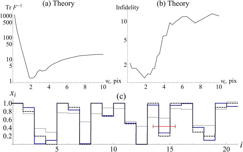
The informational approach allows us to predict the optimal correlation width of the used illumination source for the object resolution in the super-resolution regime. Intuitively, it seems that the smaller the correlation width is, the better the resolution should be. However, the analysis of the collected information shows that for the object inference perfectly correlated photons might not be the best choice. It follows from an optimization of the lower bound on the total reconstruction error. This prediction is valid for an arbitrary reconstruction method for the measurement of the second-order correlated function with both twin-photon and quasi-thermal imaging source. In Fig. 4(a) an example of the optimization is shown for the image reconstruction from a function for a pseudo-thermal state. The trace of the inverse FIM and the infidelity of the reconstruction are shown for different correlation widths . There is an optimal allowing to increase the reconstruction quality for the same number of detector counts in the super-resolution regime. One can describe the most optimal state with the following rule-of-thumb: the correlation width should be close to the smallest object details to be resolved, i.e., to the pixel size. In the super-resolution regime, the measurement of the second-order intensity correlation gives the most information per detected photon coincidence event about the object when the photons going through the neighbouring pixels are correlated. This prediction is confirmed by the experimental results shown in Fig. 4(b) using the pseudo-thermal source with various correlation widths of the generated speckles (Supplementary Note 3). A similar relation between the optimal photon correlation width and the size of the object features also holds for a SPDC source (Supplementary Note 4). For pixel size exceeding the Rayleigh limit this effect disappears; decreasing the correlation width brings about enhancement of the resolution (Fig. 4(c)).
Inference bias
The informational approach and the SWM can capture the possibility of a considerable improvement of resolution stemming from constraints imposed on the parameters. For the special case of parameters being on the borders of the allowed regions, the estimation is generally biased. The bias can significantly modify the error bounds eldarreview; eldar2004 (see Supplementary Note 5, and Fig. 4(d)). For the imaging of binary black-and-white objects (i.e., for being either 0 or 1; see bottom inset and thick lines in Fig. 4(d)), one can go far beyond the resolution limit found for grey images (top inset and thin lines in Fig. 4(d)) even without any prior assumption of the binary object structure. The reason for it is the dependence of the errors bounds on the bias derivative with respect to the parameters eldarreview. Generally, the SWM shifts the estimators near borders. The closer the estimated value is to the border, the larger is the respective shift and the error bound deviation. Notice that for the object inference demonstrated in Fig. 3, this bias effect was actually seen.
Discussion
We developed an inference method for nonlinear parametrically local problems and showed how the analysis of the information allows one to develop an estimation scheme making the complexity of the problem linear on the total number of parameters. Then, the scheme was applied to the experimental data for superresolution imaging based on higher-order correlation measurements with non-classical two-photon and pseudo-thermal states. It was shown how the FIM can be applied to optimize the imaging state for better resolution, in particular, for the correlation width of the twin-photon or pseudo-thermal imaging fields. Generally, the correlation width should be close to the smallest details to be resolved. This prediction is experimentally confirmed for measurements with pseudo-thermal light. It was also demonstrated that bias due to marginal values of estimated parameters can improve the resolution. We believe that the suggested SWM and an information approach for nonlinear inference problems will find applications for the design and optimization of inference schemes in imaging, quantum diagnostics and tomography.
Methods
The sliding windows method
The practical application of the SWM to the quantum imaging problem consists of the following steps.
First, an initial rough estimate of the object transmission amplitude is found. The pixel size is chosen in such a way that the inverse of the FIM for the reconstruction of the object, expressed in terms of pixels of the size , is diagonally dominant. The problem is strongly local and a single run of the SWM is sufficient for getting the initial estimate.
Then, the estimate is refined by representing the object in terms of smaller pixels (size ) and applying the reconstruction algorithm again. The pixel size limits the size of the object features that can be successfully reconstructed and, therefore, determines the achievable resolution.
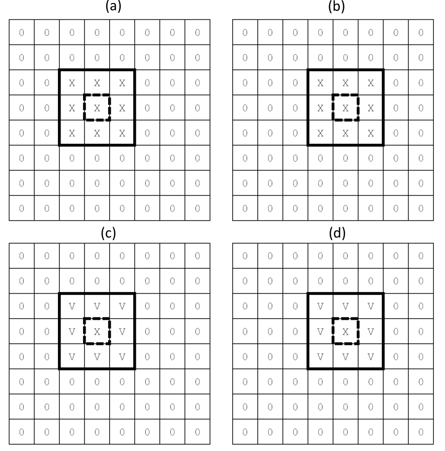
Here the pseudo code for the iterative reconstruction is presented. Both algorithms (the one for the first approximation inference and the one for refinement) are mathematically very similar, the only difference is the role of the window border: the first algorithm implies that pixels inside the border are unknown and not reliable (at each step): they need to be reconstructed but then discarded; the second algorithm implies that pixels inside the border are known (at each step) and thus can be included in the optimization problem as known constants (Fig. 5).
The pseudo code for the first approximation inference algorithm reads as follows:
For given core window dimensions, compute all core window positions which lead to the object being fully covered by non overlapping core windows.
For each position of the core window:
For a given border size, build a complete window: core + border.
Map the resulting full window to the image plane.
Find all detectors inside the obtained window in the image plane.
Combine the obtained detectors according to the order of correlations and other constraints if present.
For the obtained detector combinations, load corresponding experimental joint detection frequencies.
Build a function that maps pixels inside the full window to residual between theoretical joint detection probabilities and experimental frequencies. The theoretical probabilities are computed assuming all pixels but those inside the window to be zero.
Perform numerical minimization of the function thus obtained. Pixels inside the full window are subjected to physical constraints.
Update object pixels inside the core window with the corresponding values obtained from the minimization procedure. Discard other pixel values.
Because the algorithm first computes all core window positions and then applies one iteration per core window position, it is easily paralleled.
The pseudo code for the iterative refinement algorithm reads as follows:
For a given core window position and a given border size, build a complete window: core + border.
Map the resulting window to the image plane.
Find all detectors inside the obtained window in the image plane.
Combine the obtained detectors according to the order of correlations and other constraints if present.
For the obtained detector combinations, load corresponding experimental joint detection frequencies.
Build a function that maps pixels inside the core window to the residuals between theoretical joint detection probabilities and experimental frequencies. The theoretical probabilities are computed assuming pixels outside the core window but inside the full window to be known, they are set to constant values. Pixels outside the full window are set to zero.
Perform numerical minimization of the function thus obtained. Pixels inside the core window are subject to physical constraints.
Update pixels inside the core window with the values obtained.
Move the core window one step further.

Experiments
In the first experiment we illuminate a rotating ground glass disk (RGGD) with an attenuated, monochromatic laser operating at nm (Fig. 8). An additional lens (L1) in front of the disk allows to vary the beam waist radius at the position of the RGGD. Subsequently, we insert a far-field lens (L2) in a setting ( mm) in order to collimate the light and remove the spherical wave-front given by the point-like source. (The latter has shown to induce distortions in the subsequent imaging setup.) The object plane (OP) is then located in the far-field of the source. An object is then imaged onto the image plane (IP) by means of L3 ( mm) which is additionally endowed with a variable size pinhole (PH) to control the resolution, i.e. the Rayleigh limit of the setup. The diameter of the PH was fixed to 1.7 mm. The magnification factor of the imaging system is whereas the object distance is mm and the imaging distance is given by mm. At the image plane, photons are detected by SuperEllen, a single photon sensitive 3232 pixel SPAD array detector manufactured in CMOS technology with a pixel pitch of 44.64 m and a fill-factor of 19.7% gasparini2018; unternaehrer2018. SuperEllen is able to provide frames with a data acquisition window of 30 ns and a readout time of 10 s at a frame rate of 800 kHz. The spatial correlations between pixels were evaluated between consecutive frames with a resolution of 10 s given by the frame separation. This procedure allows for the resolution of the coherence time of the speckles of the order of s. Second- and third-order correlation functions are measured with SuperEllen.
The here presented pseudo-thermal light setup was used to obtain the following two results: Firstly, the digit “5” (Group 2) from a negative U.S. Air Force (USAF) test chart was imaged and then reconstructed from the data of a function measurement. This is shown in Fig. 3 (a) and (b) of the main text. Secondly, a negative USAF chart 3-slit pattern (Group 3, Element 2) was imaged from the object plane to the image plane for various correlation widths . The latter was modified by changing the distance between the focusing lens L1 and the RGGD and therefore the beam waist radius. Based on a measurement this allowed to demonstrate the dependence of the image reconstruction quality on the correlation width of the source shown in Fig. 4 (b) of the main text.
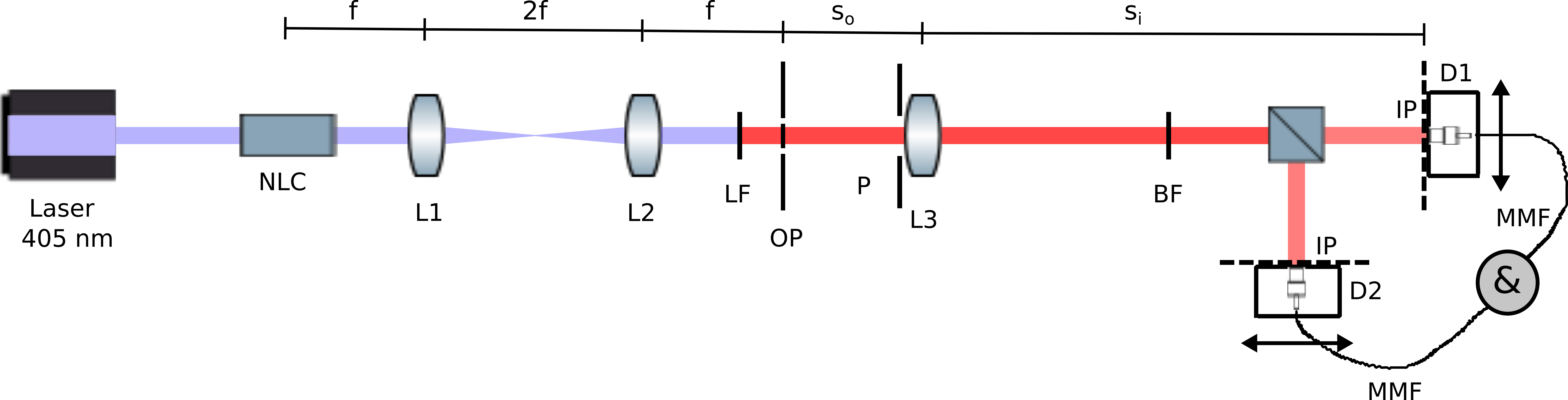
The setup for imaging with entangled photons is shown in Fig. 9. Our source generates type-0 position-momentum entangled photon states by pumping a 12 mm long PPKTP nonlinear crystal (NLC) with a continuous wave (CW) laser centered at 405 nm walborn10. The entangled photons are then emitted at 810 nm. The residual pump beam is subsequently blocked by a long-pass filter (LF) and the subsequent band-pass filter (BF) transmits photons at 810 nm with a spectral full width at half maximum (FWHM) of 10 nm to the detectors. The experimental setup contains two imaging systems: The first system consists of a 4- image using lenses and both with focal length mm. This configuration maps the entangled photon states transverse momentum distribution from the OP1 at the center of the NLC to the OP with a magnification factor of . The OP is then imaged with a single lens system onto the fiber tips of two multimode fibers (MMFs). Thereby, we have a magnification factor of for mm and mm. Both detection stages can be scanned in horizontal direction. This setup was used to record the image of a three-slit pattern of a positive USAF resolution chart (Group 4, Element 1) by measuring a second-order correlation function of the photons. The experimental correlation map and the reconstructed object can be seen in Fig. 3(c),(d) of the main text.
Data availability
The datasets generated and analysed during the current study are available from the depository of the Center for Quantum Optics and Quantum Information B. I. Stepanov Institute of Physics, National Academy of Sciences of Belarus http://master.basnet.by/Informational-approach-for.data.rar . The code itself is available upon request.
References
- (1) E. J. Candes, J. K. Romberg, and T. Tao, IEEE Trans. Inform. Theory 52, 489–509 (2006).
- (2) D. L. Donoho, IEEE Trans. Inform. Theory 52, 1289–1306 (2006).
- (3) D. Gross, Yi-Kai Liu, S. T. Flammia, S. Becker, and J. Eisert, Phys. Rev. Lett. 105, 150401 (2010).
- (4) C. A. Riofrio, D. Gross, S. T. Flammia, T. Monz, D. Nigg, R. Blatt and J. Eisert, Nat. Comm. 8, 15305 (2017).
- (5) M. Cramer, M. B. Plenio, S. T. Flammia, R. Somma, D. Gross, S. D. Bartlett, O. Landon-Cardinal, D. Poulin and Yi-Kai Liu, Nat. Comm. 1, (2010).
- (6) G. Tóth, W. Wieczorek, D. Gross, R. Krischek, C. Schwemmer, and H. Weinfurter, Phys. Rev. Lett. 105, 250403 (2010).
- (7) T. Moroder, P. Hyllus, G. Tóth, C. Schwemmer, A. Niggebaum, S. Gaile, O. Gühne, and H. Weinfurter, New J. Phys. 14, 105001 (2012).
- (8) C. Schwemmer, G. Tóth, A. Niggebaum, T. Moroder, D. Gross, O. Gühne, and H. Weinfurter, Phys. Rev. Lett. 113, 040503 (2014).
- (9) E. Thiebaut, J. Young, JOSA A 34 904 (2017).
- (10) J. M. Ortega and W. C. Rheinboldt, Iterative Solution of Nonlinear Equations in Several Variables (Academic Press Inc, San Diego, 1970).
- (11) H. R. Haffner, W. Hansel, C. F. Roos, J. Benhelm, D. Chek-al-kar, M. Chwalla, T. Korber, U. D. Rapol, M. Riebe, P. O. Schmidt, C. Becher, O. Gühne, W. Dur & R. Blatt, Nature 438, 643 (2005).
- (12) I. Bloch, J. Dalibard, & W. Zwerger, Rev. Mod. Phys. 80, 885 (2008).
- (13) J.-Ph. Tetienne, N. Dontschuk, D. A. Broadway, A. Stacey, D. A. Simpson, and L. C. L. Hollenberg, Sci. Adv. 3, e1602429 (2017).
- (14) See, for example, Y.H. Shih, IEEE Journal of Selected Topics in Quantum Electronics, IEEE 13, 1016 (2007).
- (15) J. Rehacek, D. Mogilevtsev, and Z. Hradil, Phys. Rev. Lett. 105, 010402 (2010).
- (16) M. Tsang, R. Nair, and X.-M. Lu, Phys. Rev. X 6, 031033 (2016).
- (17) R. Nair and M. Tsang, Phys. Rev. Lett. 117, 190801 (2016).
- (18) L. Motka, B. Stoklasa, M. D’Angelo, P. Facchi, A. Garuccio, Z. Hradil, S. Pascazio, F.V. Pepe, Y.S. Teo, J. Rehacek, L.L. Sanchez-Soto, The European Physical Journal Plus, 131, 130 (2016).
- (19) J. Rehacek, Z. Hradil, B. Stoklasa, M. Paur, J. Grover, A. Krzic, L.L. Sanchez-Soto, Phys. Rev. A 96 062107 (2017).
- (20) L. Seveso, M. A. C. Rossi, and M. G. A. Paris, Phys. Rev. A 95, 012111 (2017).
- (21) P. Bickel and M. Lindner, Theory Probab. Appl. 56, 1 (2012).
- (22) S. Demko, W. F. Moss, and P. W. Smith, Math. Comp., 43 491 (1984).
- (23) M. Born and E. Wolf, Principles of Optics (Cambridge University Press, Cambridge, UK, 1999).
- (24) P. Zhang, W. Gong, Xia Shen, D. Huang, and S. Han, Opt. Lett. 34, 1222 (2009).
- (25) X.-H. Chen, I.N. Agafonov, K.-H. Luo, Q. Liu, R. Xian, M.V.Chekhova, and L.-A. Wu, Opt. Lett. 53, 1166 (2010).
- (26) Y. Zhou, J. Simon, J. Liu, and Y. Shih, Phys. Rev. A 81, 043831 (2010).
- (27) D. Gatto Monticone, K. Katamadze, P. Traina, E. Moreva, J. Forneris, I. Ruo-Berchera, P. Olivero, I. P. Degiovanni, G. Brida, and M. Genovese, Phys. Rev. Lett. 113, 143602 (2014).
- (28) Y. Israel, R. Tenne, D. Oron and Y. Silberberg, Nat. Comm. 8, 14786 (2017).
- (29) R. Tenne, U. Rossman, B. Rephael, Y. Israel, A. Krupinski-Ptaszek, R. Lapkiewicz, Y. Silberberg and D. Oron, Nat. Phot. 13, 116 (2019).
- (30) A. Classen, F. Waldmann, S. Giebel, R. Schneider, D. Bhatti, Th. Mehringer, and J. von Zanthier, Phys. Rev. Lett. 117, 253601 (2016).
- (31) A. Classen, J. von Zanthier, M. O. Scully, and G. S. Agarwal, Optica 4, 580 (2017).
- (32) W. Martienssen and E. Spiller, Am. J. Phys. 32(12), 919 (1964).
- (33) J. W. Goodman, “Statistical properties of laser speckle patterns”, in Laser speckle and related phenomena, vol. 9 of Toppics in Applied Physics, J. C. Dainty, ed., (Springer, Berlin, 1975).
- (34) Y. C. Eldar, Foundations and Trends® in Signal Processing, 1 305 (2008).
- (35) Y. C. Eldar, IEEE Trans. Signal Processing, 52, 1916 (2004).
- (36) L. Gasparini, M. Zarghami, H. Xu, L. Parmesan, M. M. Garcia, M. Unternährer, B. Bessire, A. Stefanov, D. Stoppa, and M. Perenzoni, “A 3232-pixels time-resolved singlephoton image sensor with 44.64-m pitch and 19.48% fill-factor with on-chip row/frame skipping features reaching 800 khz observation rate for quantum physics applications,” in International Solid-State Circuits Conference ISSCC 18, (IEEE, 2018).
- (37) M. Unternahrer, B. Bessire, L. Gasparini, M. Perenzoni, and A. Stefanov, Optica 5(9), 1150–1154 (2018).
- (38) S. P. Walborn, C. H. Monken, S. Padua, and P. H. Ribeiro, Physics Reports 495, 87–139 (2010).
- (39) X.Q. Liu, T.Z. Huang and Y.D. Fu, Appl. Math. Lett., 19 590 (2006).
- (40) T. Politi, M. Popolizio, JIPAM 9, 31 (2008).
- (41) Zhuohong Huang, Jianzhou Liu, Applied Mathematics E-Notes, 10, 11-18 (2010).
- (42) H. WoIkowicz, G. P. H. Styan, Linear Algebra and its Applications 29, 471 (1980).
- (43) S. Emanueli, and A. Arie, Appl. Opt. 42, 6661 (2003).
- (44) J. Schneeloch, and J. C. Howell, J. Opt. 18, 053501 (2016)
Supplementary note 1. Bounds for inverses of banded and approximately banded matrices
Here we give a number of known results about inverses of banded and approximately banded matrices useful for our discussion. First of all, inverses of banded matrices can be approximated by banded matrices. For the inverse, , of the -banded matrix , one can always find such a -banded matrix such that
| (4) |
where the distance is defined as , where is the set of all -banded matrices, and the norm is defined as the maximal eigenvalue, ; is the minimal eigenvalue of the matrix apband.
Now we introduce the concept of the approximately banded matrix apband. For a given invertible matrix with we introduce sets of all -banded matrices , and the distances . We call the matrix approximately banded if distances tend to zero with increasing . For infinite matrices this condition can be formalized as
| (5) |
For infinite matrices the class of the approximately banded matrices is closed with respect to inversion. Notice that if the bandwidth of both, the direct and inverse matrices is much smaller than the matrix size, then the conclusions derived for infinite matrices will obviously hold for the finite ones. For approximately banded matrices, the bound
| (6) |
where , and
holds apband. A number of strong and illustrative results exists for inversions of strictly diagonally dominant banded matrices. The matrix is strictly diagonally dominant if . For a 1-banded (tridiagonal) real square matrix there is the bound
| (7) |
for the diagonal elements of the inverse matrix liu; tridig. For simplicity sake, here we give the coefficients , , , for the matrix with non-negative coefficients
| (8) | |||
The most remarkable observation about Eqs. (7,Supplementary note 1. Bounds for inverses of banded and approximately banded matrices) relevant for the context of this work is that the -th diagonal elements of the inverse matrix are bounded by elements of the original matrix in the vicinity . This holds for arbitrary real invertible matrix as well. Notice, that the bound Eq. (7) does not imply that the inverse matrix is close to the tridiagonal one. The similar bound exists for pentadiagonal matrices pentadig. In this case the th diagonal elements of the inverse matrix are bounded by elements of the original matrix in the vicinity .
Supplementary note 2. The Fisher information matrix and the scheme optimization
Here, we show how the error estimation given by the Cramer-Rao bound is affected by the banded structure of the Fisher information matrix (1). In a standard way, the overall performance of the image reconstruction scheme can be characterized with the lower bound on the total variance of the estimated parameters
| (9) |
The trace of the inverse matrix is majorized by the smallest eigenvalue of the Fisher matrix,
where is the eigenvalues of the matrix in Eq. (1), and is the number of parameters.
The fact that the number and value of off-diagonal elements affects the eigenvalues and the total error, can be well attested by the ”Gershgorin’s circles” theorem. It states that
| (10) |
i.e., the lower bound on the lowest eigenvalue decreases with increasing off-diagonal elements.
There is another simple and illustrative bound on the lower eigenvalue of the Fisher matrix demonstrating how the deviation of this matrix from being the diagonal one affects the error. For a general complex matrix with real eigenvalues, the bound
| (11) |
holds traces. For the trace of the squared matrix one has . So, for the constant trace, larger off-diagonal elements lead to lowering the bound in Eq. (11).
For application in near-field imaging we introduce the Fisher information matrix in the following way taking into account the physical situation. We assume that is the sum of probabilities for the object being completely transparent in the whole object plane, taking that for all images that we are considering. Then, we take all the probabilities and add the ”no counts” probability to form a complete set. For simplicity sake we assume the transmissions to be real, and write down the Fisher information matrix
| (12) |
as the sum of the matrix and the rank one matrix. Here, we can use instead of in the bound (9), since for the non-negative matrices an addition of the rank one positive matrix increases the smallest eigenvalue.
Supplementary note 3. Estimation of coefficients for near-field imaging
Here we elaborate on the coefficients connecting the registered values of the correlation function, the density matrix of the imaging state, and the characteristics of the imaging setup. The detection probabilities can be represented as polynomials on the transmissions
| (13) |
where the parameters are given by
| (14) |
and
The parameters completely describe our measurement setup. Further, they are independent of the image and they have a number of general properties stemming from the features of the point-spread function (PSF), , and the features of the field described by the density matrix .
Here, we give the parameters for the two imaging states, used experimentally, and several correlation functions.
Pseudo-thermal states
It is well-known that a rotating ground glass disk (RGGD) illuminated by a laser beam provides a pseudo-thermal light source via a randomized speckle pattern martienssen1964; goodman1975. Thereby, in the far-field of the source, the spatial correlation width , i.e. the average size of a speckle, is inversely proportional to the spatial extent of the source (the beam waist radius on the RGGD). Inside a speckle, the light is fully coherent whereas two different speckles are mutually uncorrelated. On the other hand, the coherence time of the field, i.e. the speckle lifetime, is, in addition to beam waist radius, related to the rotation velocity of the RGGD: The faster the disk rotates, the shorter becomes the coherence time of the speckle. In the following we consider coincidence measurements within the coherence time of a speckle. To estimate the actual correlation width , we measure a second-order correlation function and fit the latter by a Gaussian shape
| (15) |
where is the magnification factor of the optical system used.
In the here presented first experiment we illuminate a RGGD with an attenuated, monochromatic laser operating at nm (Fig. 8). An additional lens (L1) in front of the disk allows to vary the beam waist radius at the position of the RGGD. Subsequently, we insert a far-field lens (L2) in a setting ( mm) in order to collimate the light and remove the spherical wave-front given by the point-like source. (The latter has shown to induce distortions in the subsequent imaging setup.) The object plane (OP) is then located in the far-field of the source. An object is then imaged onto the image plane (IP) by means of L3 ( mm) which is additionally endowed with a variable size pinhole (PH) to control the resolution, i.e. the Rayleigh limit of the setup. The diameter of the PH was fixed to 1.7 mm. The magnification factor of the imaging system is whereas the object distance is mm and the imaging distance is given by mm.
At the image plane, photons are detected by SuperEllen, a single photon sensitive 3232 pixel SPAD array detector manufactured in CMOS technology with a pixel pitch of 44.64 m and a fill-factor of 19.7% gasparini2018; unternaehrer2018. SuperEllen is able to provide frames with a data acquisition window of 30 ns and a readout time of 10 s at a frame rate of 800 kHz. The spatial correlations between pixels were evaluated between consecutive frames with a resolution of 10 s given by the frame separation. This procedure allows for the resolution of the coherence time of the speckles of the order of s. Second- and third-order correlation functions are measured with SuperEllen.
The here presented pseudo-thermal light setup was used to obtain the following two results: Firstly, the digit ”5” (Group 2) from a negative USAF chart was imaged and then reconstructed from the data of a function measurement. This is shown in Fig. 3 (a) and (b) of the main text. Secondly, a negative USAF chart 3-slit pattern (Group 3, Element 2) was imaged from the object plane to the image plane for various correlation widths . The latter was modified by changing the distance between the focusing lens L1 and the RGGD and therefore the beam waist radius. Based on a measurement this allowed to demonstrate the dependence of the image reconstruction quality on the correlation width of the source shown in Fig. 4 (b) of the main text.
Assuming that the statistics of the pseudo-thermal source is Gaussian one can express the th order correlation function, measured at points , …, , as a combination of pairwise correlations
| (16) |
where represents the set of all permutations of numbers and
| (17) |
The PSF for the here discussed near-field imaging scheme is a product of the jinc function, also known as sombrero function shih,
and a phase factor
where is the first-order Bessel function, is the frequency of the imaging field and is the radius of the imaging lens. For the distances much larger than sizes of both object and image, one can take .
The representation (16) can be derived from the corresponding property of Gaussian field correlations
| (18) |
The coefficients for calculation of th order correlation function at the th set of points (, …, ) can be expressed as
| (21) |
Features of the coefficients can be illustrated with the example of small pixels, placed at points as the functions . For such basis functions, one has
| (22) |
where is the area of the pixel. The PSF diminishes with argument, i.e. tends to zero for , where is the characteristic width of the PSF, determining the Rayleigh limit. The coefficients will tend to zero with increasing of or . Our measurement scheme is therefore indeed parametrically local. An especially simple form of those locality restrictions can be obtained for a choice of object pixels in accordance with the used detection positions as : the coefficients are effectively zero for or , where is the width of the PSF expressed in terms of the object pixel size .
SPDC entangled photon states
The setup for imaging with entangled photons is shown in Fig. 9. Our source generates type-0 position-momentum entangled photon states by pumping a 12 mm long PPKTP nonlinear crystal (NLC) with a continuous wave (CW) laser centered at 405 nm walborn10. The entangled photons are then emitted at 810 nm. The residual pump beam is subsequently blocked by a long-pass filter (LF) and the subsequent band-pass filter (BF) transmits photons at 810 nm with a spectral FWHM of 10 nm to the detectors. The experimental setup contains two imaging systems: The first system consists of a 4- image using lenses and both with focal length mm. This configuration maps the entangled photon states transverse momentum distribution from the OP1 at the center of the NLC to the OP with a magnification factor of . The OP is then imaged with a single lens system onto the fiber tips of two multimode fibers (MMFs). Thereby, we have a magnification factor of for mm and mm. Both detection stages can be scanned in horizontal direction. This setup was used to record the image of a three-slit pattern of a positive USAF resolution chart (Group 4, Element 1) by measuring a second-order correlation function of the photons. The experimental correlation map and the reconstructed object can be seen in Fig. 3(c),(d) of the main text.
For this case, the probability of having simultaneous clicks of the detectors at the position and is given by
| (23) |
where can be denoted as the two-photon wavefunction shih at the detector plane given by
| (24) |
The function is denoted as the joint-position amplitude and describes the spatial correlation between photons. Ideally, for the perfectly correlated state . In practice, for the used SPDC source, one has spatial correlations approximately described by a finite weight function which also depends on the temperature of the NLC (see, for example, Refs.walborn10; arie; howell). Qualitatively, this correlation function can be approximated by a Gaussian function similar as for the pseudo-thermal state in Eq. (17) and the correlation width can be introduced in the same manner. The dependence in Eq. (24) gives us the following expression for the coefficients
with
Supplementary note 4. Optimization of resolution for the twin-photon state
In the main text, the optimization of the resolution for our near-field imaging scheme was considered for the pseudo-thermal source. It was established that there is an optimal correlation width providing for the best resolution. Here we present also results of the simulation for the SPDC twin-photon source and also an existence of the optimal correlation width. We define the correlation width as the FWHM of the spatial correlation function described in the Appendix C. Fig. 10 shows the dependence of the total variance on . Similarly to the case of pseudothermal light, there exists an optimal value of the correlation width which has the same order of magnitude as the smallest object features to be resolved. The result is not surprising, if one compares Eqs. (25) and (20) which have the same structure and differ by complex conjugation and notations for correlation function only.
Supplementary note 5. Biased estimate
Here we consider an influence of bias on the bounds for reconstruction errors. We take the set of measurements described by the probabilities , for estimation of real parameters subjected to linear inequality constraints . We assume that our reconstruction procedure provides us with the estimator , where are frequencies obtained as the outcome of our measurement device. Our estimator is taken to be biased
| (26) |
where denotes averaging over all realizations of the frequencies, , for the fixed total number of measurement runs . We denote as the vector . Notice that the bias generally depends on .
Using the definition of the bias in Eq. (26), it is easy to generalize the Cramer-Rao inequality for the lower bound on the covariance matrix
| (27) |
for biased estimators. From the Fisher information matrix (1), one can generalize the Cramer-Rao inequality deriving the following bound for the elements of the covariance matrix eldarreview
| (28) |
where is an identity matrix, and the is the bias gradient matrix with the elements
| (29) |
It is to be noted that the error bound in Eq. (28) depends only on the bias derivative, i.e., the constant bias does not influence the bound. Also, one can surmise that rapidly varying bias can strongly influence error estimations. Generally, estimation of the bias is not an easy task. The direct approach would involve estimation of the parameters for a sufficiently large number of realizations of the measurement results obtained for a large number of measurement runs. However, even some rather general considerations about the bias can be used for derivation of the bound. Here we describe the simple case of the bound given in eldar2004.
The main concept underlying the derivation of the bound is an existence of a small upper bound for the rate of bias change. Let us assume the possibility to find a number such that
| (30) |
where is the normalized vector of variables, . Then, it is possible to derive the following bound for the total error estimated as the trace of the covariance matrix
| (31) |
This simple bound is quite remarkable. It shows that for a non-singular FIM a slowly varying bias is always leading to the improvement of the error (however, notice that it is a biased estimation). Moreover, in the work eldar2004 it is proven that there is a penalized maximal likelihood estimation procedure saturating the bound in Eq. (31). Notice that the work eldar2004 also considers more complicated and refined bounds than Eq (31) based on finding the upper bound on some functions of . However, for demonstration of the border resolution enhancement in the realistic imaging scheme the simple bound given by Eq. (31) is quite sufficient.
To illustrate the influence of the estimate bias on its variance, let us consider an example of reconstructing a single parameter from the measured probabilities. Let be the single element FIM for the considered case. For example, for a binary measurement with the probabilities and of the two outcomes, the element of the FIM is . Let be the unbiased estimator for , saturating the CRB and characterized by the variance . For sufficiently large , the values of the estimator for different realizations of -measurement series are distributed according to the probability density function .
Now let us consider a constrained problem, where the inequality is imposed. To ensure the agreement of the estimated value with that requirement, one can introduce the estimator
| (32) |
The mean value of this estimator equals
| (33) |
where . For the mean value tends to the ”true” value : , and the estimate is unbiased far from the boundary value 1 (Figure 11(a)). For the estimate becomes biased.
The generalized CRB (28) for the biased estimator gives the value
| (34) |
for the variance. Far from the boundary, one has . However, for the variance of the biased estimate is twice smaller than for the unbiased estimate : (Figure 11(b)).
The total mean square reconstruction error includes both, the variance and the bias of the estimate, and can be calculated as
| (35) |
Figure 11(b) shows that, regardless of the additional systematic error introduced by the bias, the total reconstruction error for the biased estimator is smaller than for the initial unbiased estimator .
The effect can be even more pronounced for multiparameter problems. To illustrate this statement, let us consider a degenerated problem of reconstructing two parameters and when the measured signal depends on their sum only. In that case, the sum of the parameters can be estimated with a finite error , , while the error of the difference, , estimation is unbounded. The errors of estimating the parameters themselves remain unbounded as well.
Suppose that now the parameters are bounded from above: . Therefore, the sum and the difference of the parameters also satisfy the inequalities and . As soon as the ”true” values of the parameters reach the corner of the available region, , one has and . Now the estimation errors for both, the sum and the difference become finite, and the degenerate problem of finding and becomes solvable with finite accuracy.
It is worth noting, that the predicted position of the optimum at the dependence of the total variance on the correlation remains the same for unbiased (gray objects) and biased (black-and-white objects) estimates.