Pseudoscalar Meson Mixing, the Contribution of the Hadronic Continuum to Deviation from Factorization

A considerable amount of attention [1] has been devoted to the study of neutral meson mixing. In particular the matrix elements $\left\langle\bar{K^{0}}(p^{\prime})\left|\Theta_{\Delta S=2}\right|K^{0}(p)\right\rangle$[2] and $\left\langle\bar{B^{0}}(p^{\prime})\left|\Theta_{\Delta B=2}\right|B^{0}(p)\right\rangle$ [3, 5]

where $\Theta_{\Delta S=2}=(\bar{s}_{L}\gamma_{\mu}d_{L})(\bar{s}_{L}\gamma_{\mu}d_{L})$ and $\Theta_{\Delta B=2}=(\bar{b}_{L}\gamma_{\mu}d_{L})(\bar{b}_{L}\gamma_{\mu}d_{L})$ which contribute to the mass differences of the neutral mesons and in studies of CP violation have been classic subjects of investigation. The simplest approach (factorization) reduces these matrix elements to the products

deviation from factorization is described by a parameter $B$ which multiplies the above matrix elements. In factorization $B=1$.

Sophisticated calculations of $B$ appeared in the literature using quark and bag models, lattice calculations and QCD sum rule techniques.

The latter start from a 3-point function involving two pseudoscalar currents in addition to the $\Delta S$ $(\Delta B)=2$ four quark operator

Dispersion relations are written for this quantity and intermediate states inserted. The sought for matrix elements are provided by the meson poles. In addition there is a potentially large contribution arising from the pseudoscalar continuum of which not much is known.

The aim of any reliable calculation is to minimize this contribution before neglecting it.

In the case of the K-mesons the contribution of the continuum is damped by use of the Borel (Laplace) transform in which case the damping is provided by an exponential kernel $e^{\frac{-t}{M^{2}}}$. If the parameter $M^{2}$, the square of the Borel mass , is small the damping is good but the contribution of unknown higher order condensates increases rapidly. If $M^{2}$ increases the contribution of the higher order condensates decreases but the damping in the resonance region worsens. An intermediate value of $M^{2}$ has to be chosen. Because $M^{2}$ is an unphysical parameter the results should not depend on it in a relatively broad interval which is often not the case. The choice of the parameter which signals the onset of perturbative QCD is another source of uncertainty.

In the case of the B-mesons, Koerner et al. [3] use inverse powers of the dispersion variables (moments) which is legitimate because the matrix elements are infrared safe. As usual the potentially large contribution of the hadronic continuum is unknown. They estimate it by using gaps and other ill-known quantities. Recent work on B-meson mixing using Heavy Quark Effective Theory is also available [4]

In this work the aim is to practically eliminate the contribution of the hadronic continua by introducing kernels which vanish at the position of the resonances and are very small in a broad region around them.

The method will also be applied to the evaluation of the quark-gluon mixed condensate $\left\langle QGC\right\rangle=m_{0}^{2}\left\langle 0\left|\bar{q}q\right|0\right\rangle$ which enters in the calculation and to the evaluation of the K-meson decay constant.

In the Standard Model (SM) [6] the mixing of the two eigenstates of strangeness is predicted as a higher order process which contributes to the $K_{L}-K_{S}$ mass difference through the so called $\Delta S=2$ box diagram.

The $K_{L}-K_{S}$ mass difference $\Delta m$ is a sum of a long distance dispersive contribution $\Delta m_{L}$ and a short distance one $\Delta m_{S}$ proportional to the matrix element $\left\langle\bar{K^{0}}(p^{\prime})\left|\Theta_{\Delta S=-2}\right|K^{0}(p)\right\rangle$

With

Neglecting anomalous dimension factors the parameter $B$ is defined

$B=1$ in vacuum saturation and $f_{K}=.114\,GeV$

Sophisticated calculations of $B$ followed using quark and bag models, lattice calculations and QCD sum rules techniques. Unfortunately no single value for B has emerged.

Start with a 3-point function involving two pseudoscalar currents in addition to the $\Delta S=2$ four quark operator

where $j_{5}(x)=\bar{d}(x)i\gamma_{5}s(x)$ is the pseudoscalar current

Dispersion relations for this quantity are written and intermediate states inserted. The $K$-meson poles carry the sought for information in addition there is the contribution of the strange pseudoscalar continuum of which not much is known except that it is dominated by two radial excitations of the $K$, $K(1460)$ and $K(1830)$. In order to damp the unknown contribution of the continuum Borel (Laplace) transforms have been used in which case the damping is provided by an exponential kernel. As discussed in the introduction I shall proceed otherwise in order to avoid the arbitrariness and instability inherent to this method. In this work I shall use polynomial kernels in order to eliminate the contribution of the unknown continuum. The coefficients of these polynomials are chosen to make the roots coincide with the masses of the radial excitations of the K.

The amplitude $A(t=p^{2},t^{\prime}=p^{\prime 2},p.p^{\prime})$ will be studied at fixed $p.p^{\prime}$ and will be denoted by $A(t,t^{\prime})$

$A(t,t^{\prime})$ possesses a double pole, two single poles and cuts on the real $t$, $t^{\prime}$ axes extending from $th=(m_{K}+2m_{\pi})^{2}$to infinity stemming from the strange pseudoscalar intermediate states.

Consider now the double integral in the complex $t$ and $t^{\prime}$ planes

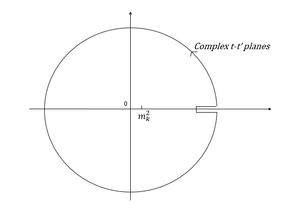
where $c$ and $c^{\prime}$ are the contours shown on Fig. 1, $f_{K}$ is the $K$ decay constant and $P(t)$ is a so far arbitrary entire function.

Because $\Phi(t),\Phi(t^{\prime})$ have no singularities inside the contours of integration the single poles do not contribute to the double integral and we are left with

The integrals over the cuts represent the contribution of the pseudoscalar strange continuum. $P(t)$ is now chosen to be a second order polynomial whose roots coincide with the masses squared of the radial excitations of the $K$, $K(1400)$ and $K(1870)$.

This choice of $P(t)$ and $P(t^{\prime})$ which vanishes at the radial excitations of the K and is very small in a very broad region around them, practically eliminates the contribution of the hadronic continuum and leaves us with the integrals on the circles of large radius $R$ where $A(t,t^{\prime})$ can be replaced by $A^{QCD}(t,t^{\prime})$ so that using $\left\langle\bar{K^{0}}\left|\Theta_{\Delta S=2}\right|K^{0}\right\rangle=\frac{16}{3}f_{K}^{2}B(p.p^{\prime})$ gives

$A^{QCD}(t,t^{\prime})$ is the sum of a factorizable and a non-factorizable part [2]

where

and

Because $B_{f}=1$, eqs. (11), (13) and (14) yield

where

Because $ln(-t)$ has a cut on the positive t-axis which starts at the origin the integral over the circle in the equation above can be transformed into an integral over the real axis so that

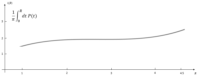
The choice of R is determined by stability considerations. It should not be too small as this would invalidate the Operator Product Expansion on the circle, nor should it be too large because $P(t)$ would start enhancing the contribution of the continuum instead of suppressing it. We seek an intermediate range of $R$ for which the integral in eq. (18) is stable.

The integral $i(R)=\int_{0}^{R}dtP(t)$ is seen to be stable for $2GeV^{2}\preceq R\preceq 4GeV^{2}$, $i(R)\eqsim.83GeV$ as shown in Fig. 2.

Then

so that

The equation above is dominated by the quark condensate term $\left\langle\bar{d}d+\bar{s}s\right\rangle$. Eq. (20) is seen to be a version of the Gell-Mann, Oakes, Renner relation [7] in the strange sector modified by $SU(3)\times SU(3)$ chiral symmetry breaking.

Turn now to the contribution of the non-factorizable part. Similar manipulations lead to

Values of $m_{0}^{2}$, which parameterizes the quark-gluon mixed condensate vary over a large range in the literature. The method presented here offers an independent evaluation of this quantity :

The integral

vanishes because the singularities inside $c$ and $c^{\prime}$ have been removed .

where $i^{\prime}(R)=\int_{0}^{R}dtP(t)(t-m_{K}^{2})$

The non-factoizable contribution is

where $i^{\prime\prime}(R)=\int_{0}^{R}dt[1+a_{1}m_{K}^{2}-(a_{1}-a_{2}m_{K}^{2})t-a_{2}t^{2}]$

The condensate $\left\langle\bar{d}d+\bar{s}s\right\rangle$ dominates our equations. It could be obtained from eq. (16), an improved calculation (to five loops) is found in [8] it gives

This,with $(m_{s}+m_{d})=(108\pm 8)\,MeV$yields $m_{0}^{2}\eqsim 1.0\,GeV^{2}$ which determines $B_{nf}$

Theoretical calculations of the weak decay constants $f_{K}$ and $f_{\pi}$ are of great interest. This has been done recently in the context of the extended Nambu-Jona-Lasinio model [9], using an improved holographic wave function [10] in the light-front quark model [11] or on lattice calculations [12].

I offer here instead a QCD calculation of $f_{K}$ to five loops. Start with the correlator

Let $\Pi(t)=\Pi^{0+1}(t)$ and consider

As before the polynomial $P(t)$ is chosen in order to eliminate the contribution of the integral on the cut. We have now to take into account the axial-vector resonances in addition to the pseudoscalar ones, i.e. $K_{1}(1273)$ and $K_{1}(1402)$ in addition to $K(1460)$ and $K(1830)$.

The choice $P(t)=1-1.42t+.648t^{2}-.093t^{3}$with the coefficients in appropriate powers of $GeV$ achieves the purpose of eliminating the contribution of the continuum. Here

The $l_{i}(t,r)$ and the strong coupling constant $a_{s}(r)$ are known to 5-loop order [15, 16] and the non perturbative condensates are given in [17]

The integral of $\Pi_{pert}(t)$ over the circle is transformed into an integral over the cut once again and finally

With the standard values $m_{s}=.10GeV^{4}$, $\left\langle a_{s}GG\right\rangle=.013GeV^{4}$, $\left\langle\bar{s}s\right\rangle=.6\left\langle\bar{q}q\right\rangle$, $\left\langle\bar{q}q\right\rangle=.02GeV^{3},$the final result is

The pion decay constant $f_{\pi}$ could also be studied. In this case data on the continuum is available from $\tau$ decay and yields $f_{\pi}$ [14]. The method used above can likewise be applied taking into account the pseudoscalar and axial-vector resonances with the result

Turn now to $\bar{B^{0}}-B^{0}$ mixing. Start with the three point correlation function

The operator $j_{B}=(m_{b}+m_{d})di\gamma_{5}b=\partial_{\mu}(d_{L}\gamma_{\mu}\gamma_{5}b_{L})$ is the interpolating current for the $B$ meson and $\left\langle 0\left|j_{B}(0)\right|B^{0}\right\rangle=f_{B}m_{B}^{2}$

The relevant quantity to calculate is the matrix element $A=\left\langle\bar{B^{0}}\left|O(\mu)\right|B^{0}\right\rangle$ where $O(\mu)=(b_{L}\gamma_{\mu}d_{L})(d_{L}\gamma_{\mu}b_{L})$ is the local 4-quark operator at the normalization point $\mu$ which can be used to evaluate the splitting of heavy and light mass eigenstates. The simplest approach (factorization) [6] reduces $A$ to

where $\left\langle 0\left|\bar{b}_{L}\gamma_{\mu}\gamma_{5}d_{L}\right|B^{0}(p)\right\rangle=if_{B}p_{\mu}$

The deviation from factorization is again parametrized by $B_{B}$ defined as $A=B_{B}A^{f}$. In factorization $B_{B}=1$.

A nice way to calculate $B$, using inverse moments, was used in [3]. In the present work I shall follow their approach but the contribution of the higher resonances and continuum shall be estimated in a different less model dependent and more reliable way.

A dispersion representation of the correlator reads

where $q=p_{1}-p_{2}$. Consider the moments of the correlation function at $p_{1}^{2}=p_{2}^{2}=q^{2}=0$

Because the origin is infrared safe $M_{ij}$ can be computed in QCD [13]. It also has a phenomenoligical representation

where the ellipses stand for the contribution of the higher resonances and the continuum. Separating the factorizable part we obtain two sum rules

The l.h.s of the above eqs. represent the phenomenology and the r.h.s the QCD theoretical expressions.

The $\Delta^{\prime}$s are the contributions of the higher resonances and the continuum. While [3] try to estimate their contribution using gaps and other ill-known parameters, I aim to eliminate it altogether.

For this purpose note that the integrals in eq. (40) are fast convergent so that the bulk of the contribution to the continuum come from the vicinity of the first resonance. If this contribution is eliminated $\Delta_{ij}$ and $\Delta^{\prime}_{ij}$ become negligible and can be discarded. This is done by using instead of eq. (40)

If $m^{\prime}$ is close to the mass of the first resonance, the factor ($\frac{m^{\prime 2}}{t}$ -1) annihilates the integrand in its vicinity. Because of the fast convergence due to the denominators the main contribution of the continuum is eliminated and this justifies the neglect of $\Delta$ and $\Delta^{\prime}$.

Taking $i=j=2$ eqs. (42) become

or

The $M$s are the theoretical QCD values and the $M^{f}$ their factorizable counterparts.

It was found in [3] that

Expressions for $M_{ij}^{non-perturbative}$ are given in [13]. In the present approach their contribution vanishes. The quantities $a_{ij}$, $b_{ij}^{f}$ , $b_{ij}^{nf}$ represent the LO, NLO and non-factorizable contributions.

Then, if

The corresponding expression in the work of [3] is

Where $\delta R$ and $\delta C$ are parameters which account for the resonances and continuum contribution and which they estimate by fitting and using gap parameters. The present approach avoids this arbitrariness.

The $a_{ij}$ are

which yields

The $b_{ij}^{nf}$ are given in [3]

The Particle Data Group lists two candidates for $m^{\prime}$, $m^{\prime}(5.84)$ and $m^{\prime}(5.97)$. A reasonable choice is then $(\frac{m^{\prime}}{m_{b}})^{{}^{2}}=2.0$ which yields $\frac{a_{s}}{4}\delta=-.006$ or $B_{B}\simeq 1.0$

Deviation from factorization is negligible.

In this work i have studied the contribution of the hadronic continuum to deviations from factorization in neutral K and B meson mixing. In both cases I minimized this contribution before neglecting it by using simple kernels in the dispersion integrals which vanish at the low lying resonances, in the case of the K-meson a polynomial kernel was used, the same method (and kernel ) was also used in the calculation of the quark- gluon mixed condensate as well as the evaluation of the K-meson decay coupling constant $f_{K}$.

For the B-meson inverse moments were used. These render the integrals fast convergent and concentrate the contribution to the dispersion integral in the vicinity of the first resonance. In this case the kernel used is of the form $(\frac{m^{\prime 2}}{t}-1)$ where $m^{\prime}$ lies in the vicinity of the first resonance.

This method avoids the arbitrariness and instability inherent to previously used ones.

References

• [1] See e.g: Ulrich Nierste, arXiv:0904.1869
• [2] I. Picek, Desy 86.036 (1988), R. Decker, Nucl. Phys. B227, 66 (1986), L. J. Reinders and S. Yazaki, Nucl. Phys. B288, 789 (1987), N. Bilic, C. A. Dominguez and B. Guberina, Z. Phys. C39, 355 (1988), N. Papadopoulos and H. Vogel, Z. Phys. C51, 73 (1991), E. Braaten, S. Narison and A. Pich, Nucl. Phys. B373, 581(1992)
• [3] J. G. Korner, A. I. Onishchenko, A. A. Petrov and A. A. Pivovarov, Phys. Rev. Lett. 91, 192002 (2003)
• [4] D. King, A. Lenz and T. Rauh, arXiv:1904.00940, M. Kirk, A. Lenz and T. Rauh, arXiv:1711.02100
• [5] S. Aoki, Flag Working Group, arXiv:1607.00299
• [6] S. L. Glashow, Nucl. Phys. 579 (1961), S. Weinberg, Phys. Rev. Lett. 19, 1264 (1967), M. K. Gaillard and B. W. Lee, Phys. Rev. D397 (1974)
• [7] M. Gell-Mann, R. J. Oakes and B. Renner, Phys. Rev. 175, 2195 (1968)
• [8] C. A. Dominguez, N. F. Nasrallah and K. Schilcher, JHEP 0802, 072 (2008)
• [9] M. K.Volkov, K. Nurlan and A. A. Pivovarov, arXiv:1906.06680
• [10] Q. Chang, X. N. Li, X. Q. Li and F. Su, Chin. Phys. C42, 073102 (2018)
• [11] H. M. Choi and C. R. Ji, Phys. Rev. D75, 034019 (2007)
• [12] N. Carrasco et al., Phys. Rev. D91, 054507 (2015)
• [13] A. A. Pivovarov, arXiv:9606.482
• [13] M. A. Shifman, A. I. Vainshtein, V. I. Zakharov, Nucl. Phys. B147 (1979)
• [14] C. A. Dominguez, N. F. Nasrallah and K. Schilcher, Phys. Rev. D80, 054014 (2009)
• [15] K. G. Chetyrkin, B. A. Kniehl and M. Steinhauser, Phys. Rev. Lett. 79, 2184 (1997)
• [16] P. A. Baikov, K. G. Chetyrkin and J. H. Kuhn. Phys. Rev. Lett. 101, 012002 (2008)
• [17] E. Braaten, S. Narison and A. Pich, Nucl. Phys. B373, 581 (1992)