A lognormal type stochastic volatility model with quadratic driftWe thank Damien Ackerer for helpful comments.
Abstract
This paper presents a novel one-factor stochastic volatility model where the instantaneous volatility of the asset log-return is a diffusion with a quadratic drift and a linear dispersion function. The instantaneous volatility mean reverts around a constant level, with a speed of mean reversion that is affine in the instantaneous volatility level. The steady-state distribution of the instantaneous volatility belongs to the class of Generalized Inverse Gaussian distributions. We show that the quadratic term in the drift is crucial to avoid moment explosions and to preserve the martingale property of the stock price process. Using a conveniently chosen change of measure, we relate the model to the class of polynomial diffusions. This remarkable relation allows us to develop a highly accurate option price approximation technique based on orthogonal polynomial expansions.
1 Introduction
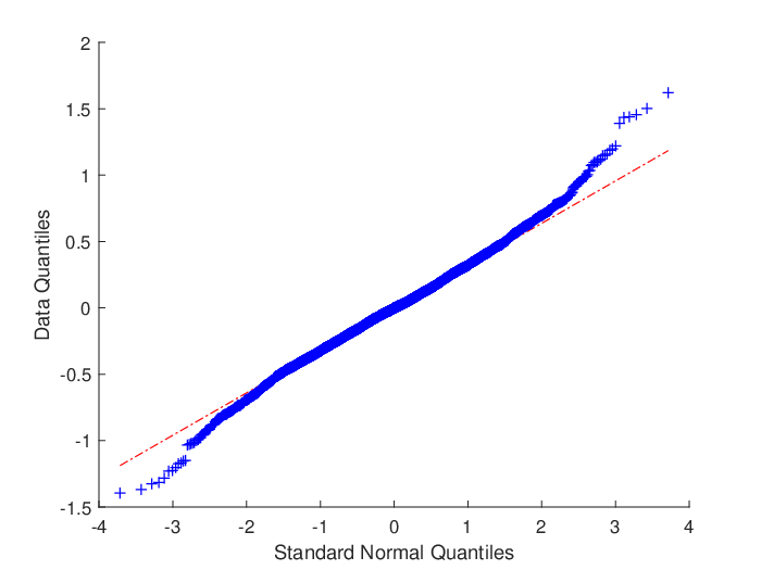
The popularity of the Heston 1993 model and, more generally, affine models (see e.g., Duffie et al. 2003) for modeling stochastic volatility is in large part due to their analytical tractability. However, there is abundant empirical evidence that favours non-affine models, in particular specifications with a lognormal type of diffusion for the (instantaneous) volatility.11 1 With lognormal type of diffusion we mean a diffusion with , for some . For instance, Christoffersen et al. 2010 show that absolute changes in realized volatility are positively correlated with the volatility level and do not follow a Gaussian distribution. In contrast, the Heston model implies that (instantaneous) changes in volatility should be Gaussian and independent of the volatility level. Changes in the log realized volatility, on the other hand, closely resemble a normal distribution, which motivates the use of a lognormal type of diffusion component in the volatility process.22 2 See Christoffersen et al. 2010 for the S&P500 index, Andersen et al. 2001 for individual stocks in the DJIA index, and Andersen et al. 2001 for foreign exchange markets. Figure 1 reproduces these results using a 5-minute sub-sampled daily realized volatility measure for the S&P500 index from January 2000 until June 2019 and confirms the findings of Christoffersen et al. 2010.
Lognormal type stochastic volatility models are, however, particularly prone to problems such as moment explosions and loss of the martingale property for the asset price, see e.g. Lions and Musiela 2007 and Andersen and Piterbarg 2007. These problems are caused by the fat right tail of the volatility distribution, which can cause large spikes in the asset price. Having finite higher order moments for the asset price is important, for example, to price derivatives with a super-linear payoff. Andersen and Piterbarg 2007 highlight the importance of these type of derivatives in interest rate markets. Moreover, when pricing derivatives with Monte-Carlo simulations, the payoff needs to have a finite second moment in order to use the central limit theorem to derive confidence intervals on the Monte-Carlo estimators. For example, if the volatility process has an affine drift and a linear dispersion function, then the instantaneous correlation between log-price and volatility has to be smaller than in order for the asset price to have a finite fourth moment. In this paper, we propose a novel non-affine one-factor stochastic volatility model featuring a diffusion with a quadratic drift function and a linear dispersion function for the volatility process. The quadratic term has a negative coefficient in our model, which allows for a rapid reduction following an upward spike in the volatility.33 3 Bakshi et al. 2006 find empirical evidence for stochastic volatility models with nonlinear drift. In particular, they find a significantly negative coefficient on the quadratic term in the drift. The linear dispersion function produces lognormal type innovations in the volatility and the quadratic term in the drift controls undesirable side effects such as moment explosions and loss of martingality. Moreover, using the critical moment formula of Lee 2004, we show that a nonzero quadratic term in the drift allows to control both the small strike and large strike tail of the Black-Scholes implied volatility skew. The volatility process in our model is stationary and has a Generalized Inverse Gaussian (GIG) distribution as steady-state distribution. The GIG distribution, which contains the inverse Gaussian, hyperbolic, gamma, and inverse-gamma as special cases, has broad empirical support for modeling stochastic volatility in stock returns, see for example Barndorff-Nielsen 1997, Eberlein 2001, Eberlein and Prause 2002, and Gander and Stephens 2007.
Since our model is far from affine, tractability is not straightforward. If we set the quadratic term in the drift of the volatility to zero, then our model fits in the class of polynomial diffusions, see e.g. Filipović and Larsson 2016. This class of stochastic processes, which contains all affine diffusions as special cases, is characterized by the fact that their infinitesimal generator maps polynomials to polynomials of the same degree or less. As a consequence, all conditional moments of the log-asset price are available in closed form and European style derivatives on the asset price can be priced using moment-based approximation methods, see e.g. Ackerer and Filipović 2019.44 4 For applications of polynomial processes in derivative pricing, see for example Filipović et al. 2016, Ackerer and Filipović 2016, Filipović and Willems 2017, Ackerer et al. 2018, and Willems 2019. The polynomial property is lost, however, as soon as we have a nonzero quadratic term in the drift of the volatility. We circumvent this problem by introducing a change of measure under which the polynomial property is recovered. Under the new measure, derivative prices are given by the expectation of the discounted payoff multiplied by the Radon-Nikodym density of the measure change. We show how to compute all joint conditional moments of the log-asset price and log-Radon-Nikodym density in closed form under the new measure. An orthogonal polynomial expansion technique in the spirit of Ackerer and Filipović 2019 then allows us to efficiently price European style derivatives on the asset price.
The remaining of this paper is structured as follows. Section 2 describes the model dynamics and Section 3 analyzes the steady-state distribution of the volatility process. In Section 4 we study the problem of moment explosions. Section 5 relates our model to the class of polynomial diffusions, which is used in Section 6 to develop a derivative pricing approximation method. Section 7 contains a numerical study of the model and Section 8 concludes. All proofs and additional technical results are collected in the Appendix.


2 Model specification
We consider a financial market modeled on a filtered probability space , where is a risk-neutral probability measure. Henceforth denotes the -conditional -expectation. Let denote the stock price and assume for simplicity zero interest rates and no dividend payments.55 5 Alternatively, one can also think of as, for example, an interest rate variable (e.g., forward rate or swap rate) and replace by the appropriate pricing measure. We specify the following -dynamics for the log-price
| (1) | ||||
| (2) |
with , , , , and independent -Brownian motions. The volatility process mean-reverts around a constant level with a stochastic speed of mean-reversion . Our model specification nests many existing models. The lognormal SABR model of Hagan et al. 2002 arises when , in which case is simply a geometric Brownian motion without drift. In this case, however, the volatility process is not mean-reverting, which is an important empirical feature. If we set and , then becomes a mean-reverting diffusion with affine drift and linear dispersion function, which we refer to as a linear diffusion. This type of model has been studied in Lewis 2000, Karasinski and Sepp 2012, Sepp 2014; Sepp 2016, Lee et al. 2016, and Ackerer and Filipović 2019.66 6 Also related is the GARCH diffusion model of Nelson 1990 and Barone-Adesi et al. 2005, where is modeled as a diffusion with affine drift and linear dispersion function. Applying Itô’s lemma shows that the corresponding volatility process also has a linear dispersion function, but it does not have an affine drift. Directly modeling volatility seems more intuitive and provides a more natural interpretation for the model parameters. For and , equation (2) is known as the logistic diffusion and originated in the context of modeling constrained population growth in biology, see e.g. Tuckwell and Koziol 1987.77 7 The deterministic version of this SDE was developed in the early 19th century by the Belgian mathematician Pierre Frano̧is Verhulst to model population growth. In the context of finance, the logistic diffusion has been used, for example, in a general equilibrium model by Merton 1975 and in a stochastic volatility model by Hull and White 1987 and Lewis 2019.88 8 Hull and White 1987 specify for some parameters . Applying Itô’s lemma shows that follows a logistic diffusion: .
The following proposition shows that the model is well defined and that zero is an unattainable boundary for .
From the proof of Proposition 2.1, it becomes clear that the non-negativity assumption is crucial in order for (2) to have a global solution, cf. Remark A.1. Indeed, if , then blows up in finite time.
Remark 2.2.
Although zero is a natural lower bound for the volatility process, we can generalize (2) by adding a lower bound as follows
with and the same restrictions on the other parameters as before. All the results we derive in our paper are easily adjusted to accommodate this generalization.
3 Steady-state distribution of
In this following proposition, we explicitly derive the steady-state distribution of .
Proposition 3.1.
If either , or and , then the process has a steady-state distribution with density function
where . If and , then a.s. as .
The steady-state distribution therefore belongs to the class of Generalized Inverse Gaussian distributions, see e.g. Jorgensen 1982. The integration constant such that integrates to one is provided in the proof (see Section A.2). We distinguish four different cases, based on the values for and :
- 1.
For , the process becomes a geometric Brownian motion without drift, which goes to zero almost surely as .
- 2.
For and , the process becomes a linear diffusion and we recover the inverse gamma distribution as steady-state distribution, see e.g. Barone-Adesi et al. 2005. The first moment of is equal to , so that can be interpreted as the long-term level of mean reversion. Higher order moments do not always exist because the inverse gamma distribution has a right tail with polynomial decay. Remark that , regardless of and , due to the exponential decay of of the left tail.
- 3.
For and , the process becomes a logistic diffusion. If , then a similar behavior as in the first case occurs and almost surely as . If , we recover the gamma distribution as steady-state distribution, which has finite moments of any order. In particular, the first moment equals . As highlighted in Merton 1975 and Ewald and Yang 2007, we can therefore no longer interpret as the long-term level of mean reversion. Remark that if and only if .
- 4.
For , the steady-state distribution has a gamma tail on the right and an inverse gamma tail on the left. As a consequence, has finite moments of any order and . In particular, the first moment equals (see e.g., Jorgensen 1982)
where denotes the modified Bessel function of the second kind.99 9 In Appendix B.1 we provide a tight lower bound (based on Jensen’s inequality) for the first moment of the steady-state distribution that does not involve any special functions. In general, the first moment of the steady-state distribution will not be exactly equal to , so we can not interpret as the long-term level of mean-reversion. However, the difference is small for standard parameterizations.
4 Moment explosions
In this section, we build on the general findings of Lions and Musiela 2007 to investigate moment explosions of the stock price in our model. In order to use (1)-(2) for option pricing, we need to be a -martingale. The following proposition derives a necessary and sufficient condition.
Proposition 4.1.
is a -martingale if and only if .
If , then is a -martingale if and only if , which is a well known problem with this type of model. While equity markets generally feature a negative correlation between stock returns and volatility, other applications might require a positive correlation. Proposition 4.1 shows that our model can accommodate a positive correlation if is sufficiently large. In particular, if , then is always a -martingale in our model, regardless of . Intuitively, the quadratic drift term has a stabilizing effect on the volatility because the speed of mean reversion becomes very large at high volatility levels.
Andersen and Piterbarg 2007 highlight the importance for to have finite moments greater than one for pricing contracts with super-linear payoff, which occur frequently in interest rate derivatives markets. Examples include CMS swaps, in-arrears swaps, and Eurodollar futures. Moreover, when using Monte-Carlo simulations to find the price of a derivative, the payoff needs to have finite second order moment in order to derive confidence intervals on the Monte-Carlo estimator with the central limit theorem. The following proposition derives a lower bound on such that has finite moments of a given order.
Proposition 4.2.
Let .
- 1.
If , then
If , then the statement is also true for .
- 2.
If , then
In particular, if and , then is finite if and only if . A negative correlation has a dampening effect on the moments of the return process, however it must be sufficiently negative in this case for higher moments to exist. For instance, already for we require in case , which can be quite restrictive. Proposition 4.2 shows that the quadratic term in the drift of can take over the role of the negative correlation to stabilize the moments of the return process, which allows the correlation to remain a free parameter. Remark also that for and , we have , regardless of .
The seminal work of Lee 2004 relates moment explosions to the asymptotic behaviour of the Black-Scholes implied volatility smile as a function of log-moneyness. Specifically, define the critical moments
| (3) |
Remark that Proposition 4.2 implies in particular that the critical moments in our model do not depend on the time horizon , so henceforth we omit the time argument and simply write . Let denote the Black-Scholes implied volatility of a European call option with time-to-maturity and strike price . Using the formulation of Keller-Ressel 2011, the critical moment formula of Lee 2004 states
| (4) |
where we define the decreasing function . The critical moments in our model can directly be computed using the result of Proposition 4.2, as shown in the following corollary. Note that Black-Scholes implied volatility only makes sense if is a -martingale, so we only consider the case , cf. Proposition 4.1.
Corollary 4.3.
Suppose is a -martingale, i.e., .
- 1.
If , then
(5) - 2.
If , then and .
- 3.
If , then and .
The critical moment formula (4) and Corollary 4.3 give us important information about the tail behaviour of in our model. If , then the critical moments are finite, which implies asymptotically linear behaviour of in for all . The slope of the small and large strike tail is controlled by both and . For , we get in particular and . In this case, only controls the slope of large strike tail, while the slope of the small strike tail is always equal to . With as a free parameter, we can therefore more accurately capture both the small and the large strike tail of the Black-Scholes implied volatility skew.
Remark 4.4.
As noted by Lee 2004, the critical moment formula (4) can be useful to facilitate model calibration. Suppose we observe a Black-Scholes implied volatility skew for a range of strikes and a certain maturity . From the smallest and largest strike, we can approximately infer and , respectively.1010 10 Remark that in our model, the critical moments do not depend on the time horizon, while the implied critical moments will likely not be exactly equal for different option maturities, in which case we can for example average the implied critical moments across maturities. The parameters and can then be calibrated to these implied critical moments using (5). This approach should be seen as a way to get good initial guesses for and .
We end this section with an additional result on the two extreme correlation cases.
Proposition 4.5.
- 1.
If and , then
- 2.
If , , and , then
For , we know from Proposition 4.1 that is a -martingale and from Proposition 4.2 that for all and all . If moreover , then Proposition 4.5 shows that the stock price becomes bounded form above. Remark that this additional condition is trivially satisfied when . For , the stock price is a -martingale if and only if , see Proposition 4.1. From Proposition 4.2 we have in this case for all and all . If moreover , then the stock price has a lower bound strictly larger than zero. Remark that these results are consistent with the critical moments derived in Corollary 4.3.
5 A polynomial diffusion in disguise
In this section we show how our model can be related to the class of polynomial diffusions using a conveniently chosen change of measure.
Define the process through the following stochastic differential equation (SDE)
| (6) |
with . Fix a time horizon and define the probability measure through the following Radon-Nikodym derivative
| (7) |
Remark if . The following proposition shows that the change of measure is well defined.
Proposition 5.1.
The process is a -martingale.
Henceforth denotes the -conditional -expectation. By Girsanov’s theorem we have that
are independent -Brownian motions. The -dynamics of becomes
| (8) |
The quadratic term in the drift of vanishes and becomes a polynomial diffusion under . Indeed, it has an affine drift and a linear dispersion function, so that its infinitesimal generator maps polynomials to polynomials of the same degree or less. This allows us to compute all -moments of in closed form, which is informative about the -distribution of . For derivative pricing purposes (see Section 6 for more details), we are not particularly interested in the -distribution of . Instead, we are mainly interested in the -distribution of or, equivalently, in the joint -distribution of and . The process is not a polynomial diffusion under , because the drift of and contains a quadratic term :
However, by augmenting the state with , we can see that jointly becomes a polynomial diffusion under since has the following dynamics
This observation makes it possible to calculate all conditional -moments of in closed form. Before we do this, we first introduce some notation. Denote for by the space of polynomials on with total degree at most . Define the subspace of trivariate polynomials as
where denotes the total degree of a polynomial. The following lemma provides the dimension of , i.e. the number of linearly independent polynomials in .
Lemma 5.2.
The dimension of is
The following proposition provides an explicit formula for the conditional -moments of , which will be the cornerstone of the derivative pricing approximation method in Section 6.
Proposition 5.3.
The infinitesimal generator of the process under leaves invariant. That is, there exists a matrix , such that , where denotes a vector of polynomial basis functions for . As a consequence, we have for any
| (9) |
The matrix is straightforward to construct in practice by choosing to be a monomial basis and then collecting terms according to their exponents in the vector of polynomials , see equation (22) in the Appendix.
6 Derivative pricing
In this section we show how European style derivatives on the stock price can efficiently be computed using the available -moments of .
6.1 Polynomial payoff approximation
Consider a derivative on the stock price with payoff at time , for some integrable payoff function . The price at time is given by
| (10) |
The auxiliary process can therefore be interpreted as a stochastic discount rate under the new measure. The positive correlation between and provides a dampening effect on the ‘discounted’ payoff under the new measure, which is the equivalent of the dampening effect of the quadratic drift term of that disappeared with the measure change.
The conditional -distribution of is not known, but we do know all the conditional -moments of thanks to the moment formula (9). Therefore, we can approximate the derivative price by approximating the function with a polynomial , for some . We would like the polynomial approximation to be most accurate for the values that is most likely to take under , since they contribute the most to the right hand side of (10). This motivates the following least-squares approach to determine the approximating polynomial
| (11) |
where is an auxiliary probability density function which proxies the unknown -density of .1111 11 We assume that is such that the double integral in (11) is finite for all . Put differently, is the orthogonal projection of on the space of bivariate polynomials of total degree or less in a weighted Hilbert function space with weight . If we denote by the vector representation of with respect to the basis , the option price approximation becomes
| (12) |
In Section 6.2 we show how to choose and in Section 6.3 we solve the optimization problem in (11).
6.2 The auxiliary density
It remains to choose a good auxiliary density . We use an approach that closely resembles the Gaussian mixture specification of Ackerer and Filipović 2019. Conditional on the trajectory , the -density function of the random variable can be formally written as
where denotes the density function of a Gaussian distribution with mean and variance , denotes the Dirac delta function, and
The true -density function of can therefore be expressed as
We specify the auxiliary density as
| (13) |
where , , , , are constants to be determined subject to . The quadruplets represent a discretization of the -distribution of in mass points, which can be obtained by discretizing the single source of uncertainty . Specifically, we use the IJK scheme of Kahl and Jäckel 2006 with equidistant time steps to obtain the following discretization scheme for , , , and :
where is the step size, is a -dimensional standard normal random variable, and , , , . If we are given weighted samples , , of the random variable , then by plugging them into the above scheme we obtain the quadruplets . As highlighted by Ackerer and Filipović 2019, raw Monte-Carlo simulation with requires far too many samples to produce an accurate approximation of the distribution. Instead, deterministic discretizations of the -dimensional standard normal distribution, such as the quantization techniques of Pagès and Printems 2003 or Gaussian cubature rules, are preferred in order to keep small. In the numerical study in Section 7, we use the multivariate Gauss-Hermite quadrature method described in Jäckel 2005 to obtain the weighted samples . The advantage of Gauss-Hermite quadrature is that the tails of the distribution are accurately captured, which is important for the stability of our approximation method as , the total polynomial degree of the approximation, increases.
6.3 The optimal polynomial
Now that we have specified the auxiliary density function, we can solve the optimization problem in (11). Denote by , , a vector of polynomial basis functions for . We can rewrite (11) as
| (14) |
Proposition 6.1.
Without loss of generality, we assume that is a monomial basis with , for exponents such that , . Plugging (13) in the expression for in (15) gives
The remaining integral is simply the -th moment of the univivariate Gaussian distribution, which is known in closed form.1212 12 In Appendix B.2 we provide a simple formula for the moments of the Gaussian distribution. The elements of the vector become
| (16) |
In general, the integral in (16) has to be computed numerically, for example using Gauss-Hermite quadrature. For specific payoff functions, the integral can be computed in closed form. For example, the following proposition derives a recursive formula for the case of a European call option.
Proposition 6.2.
Suppose , for some . The integral
satisfies the following recursion for
with , the standard normal density, and starting values
with the standard normal cumulative distribution function.
7 Numerical study
In this section we investigate the numerical accuracy of the option price approximation proposed in the previous section.
We set the model parameters as , , , , . These are realistic parameters that produce a volatility process with strong mean-reversion and a high volatility of volatility that can cause occasional spikes, see for example Figure 2 for a simulated (under ) trajectory. Consider a European call option with time-to-maturity and log-strike . Figure 3(a) and 3(b) plot the option price approximations for ranging from 1 to 10. We set , and use the Gauss-Hermite quadrature rule to obtain a discretization of the univariate standard normal distribution in points. As a benchmark, we also run a Monte-Carlo simulation with sample paths.1313 13 We use a quadratic polynomial approximation of the discounted payoff as a control variate to substantially reduce the variance of the Monte-Carlo estimator. To determine the polynomial approximation, we perform a linear regression with the simulated trajectories. This is similar to the polynomial approximation in Section 6, where we now use the simulated empirical distribution as auxiliary distribution. For all strikes and maturities considered, converges to within the confidence bands of the Monte-Carlo estimator with . For , the pricing error is most noticeable for the low strike option (i.e., the in-the-money call). This is not surprising, since the true log-return distribution is negatively skewed (). Therefore, approximations which do not take into account at least third order moments will be far off for low strike options. The results are robust to changes in the number of discretization points , as long as it is not too small. If is chosen very small (say, ), then the approximation blows up for larger . Intuitively, for small the auxiliary distribution has very thin tails and the polynomial approximation of the discounted payoff will therefore only be accurate over a small domain. Since the true probability distribution assigns considerable weight outside of this domain, the polynomial approximation will blow up quickly. In Figure 3(c) and 3(d), we do the same exercise with . For the auxiliary distribution, we use the Gauss-Hermite quadrature rule with 15 points in each dimension, which gives a total of points.1414 14 Using the pruning method described in Jäckel 2005, we can reduce the number of discretization points to 185 by omitting the ‘corner’ points that carry a very small weight. Compared to the case , the approximations converges faster to the true price. However, this comes at a computational cost because the number of discretization points in the auxiliary distribution is much larger.


8 Conclusion
We have introduced a new stochastic volatility model featuring a volatility process with a quadratic drift and a linear dispersion function. We have shown that the quadratic term in the drift is important to control moment explosions in the stock price and, in particular, the small strike tail of the Black-Scholes implied volatility skew. The volatility process has a stationary distribution that belongs to the class of Generalized Inverse Gaussian distributions, which arises frequently in the empirical literature on volatility modeling. In order to make the model tractable, we introduced a change of measure such that the model fits into the class of polynomial diffusions, which opened the door to polynomial expansion methods to accurately approximate option prices.
Appendix A Proofs
A.1 Proof of Proposition 2.1
We start by showing that (2) has a unique -valued solution. We denote by
the drift and dispersion function of , respectively. Since and are polynomials, they are in particular locally Lipschitz continuous. Hence, strong uniqueness holds for solutions of (2), see e.g. (Karatzas and Shreve 1991, Theorem 2.5). The dispersion function satisfies a linear growth condition
for . The drift function does not satisfy a linear growth condition, so the classical existence result of Itô (see e.g., (Karatzas and Shreve 1991, Theorem 2.9)) does not apply. However, since the quadratic term in has a negative coefficient, does satisfy
for some . Hence, there exists a unique global solution to (2), cf. (Kloeden and Platen 1995, Chapter 4.5, p.135). It remains to verify that the solution stays in , which we proof using a comparison theorem. Consider the logistic diffusion
| (17) |
This SDE has a unique solution given by
Notice that, since , we have for all . Using a comparison theorem (Ikeda and Watanabe 1989, Chapter VI, Theorem 1.1) and gives a.s. for all .
Remark A.1.
Notice that, if , then explodes in finite time and therefore as well. The assumption is therefore crucial to guarantee existence of a global solution.
Next, we show that the stochastic integrals in (1) are well defined by showing that
To this end, consider the SDE
which has as unique solution. Using a comparison theorem (Ikeda and Watanabe 1989, Chapter VI, Theorem 1.1) and gives a.s. for all . Since is a polynomial diffusion, it has finite moments of any order. Therefore we have
From the comparison arguments used in first and second part of this proof, we also obtain the following pathwise bounds on
| (18) |
A.2 Proof of Proposition 3.1
Using the Fokker-Planck equation we have that must satisfy the following second order linear ODE
Making the Ansatz , for some constants , , and , and collecting terms gives
where is a constant to be determined such that integrates to one.
Remark A.2.
The motivation for this Ansatz comes from the special cases and . If , then is a GARCH diffusion, which is known to have the inverse gamma distribution as steady-state distribution. If , then is a logistic diffusion, which is known to have the gamma distribution as steady-state distribution if . Therefore, the steady-state distribution of must contain the gamma and inverse gamma distribution as special cases.
If , then is a generalized inverse Gaussian distribution and the normalization constant becomes (see e.g., Jorgensen 1982)
where denotes the modified Bessel function of the second kind. If and , then is a gamma density and therefore becomes
where denotes the gamma function. Note that the condition is equivalent to .
For and , recall from (18) that we have almost surely the following upper bound
If , then a.s. for and therefore we have a.s. for .
A.3 Proof of Proposition 4.1
By Theorem 2.4(i) in Lions and Musiela 2007, is a -martingale if
The limit can be rewritten as
Therefore, is a -martingale if . Indeed, if the limit is and if the limit is .
Conversely, by Theorem 2.4(ii) in Lions and Musiela 2007, is not a -martingale if
for some smooth, positive, and increasing function such that , . Choosing gives
Therefore, is not a -martingale if .
A.4 Proof of Proposition 4.2
- 1.
By Theorem 2.5 in Lions and Musiela 2007, we need to show that there exists an such that1515 15 The paper of Lions and Musiela 2007 contains some typos that are relevant for the derivation of this proof. Specifically, in equation (26), the function should be defined as instead of . In equation (28), the in the last term has to be replaced by .
(19) The limit can be rewritten as
(20) Define the parabola . If
then has two distinct positive roots
From (20) it becomes clear that if we pick , then (19) is satisfied.
- 2.
Follows directly from Theorem 2.6 in Lions and Musiela 2007 and
A.5 Proof of Corollary 4.3
Define the function on . It is readily verified that is increasing on with and decreasing on with .
If , then standard calculations show , so by Proposition 4.2 there must be a critical moment both in and in . In order to find the critical moments, we have to solve the equation
| (21) |
Squaring both sides shows that a critical moment has to satisfy
If , then is a convex parabola with and , where the second inequality follows from the assumption that . Therefore, has two real roots
with and . It is directly verified that solves (21).
If , then . Therefore, for all , so that . Since , there will be a critical moment in and it is given by the single root of :
Similarly, if , then . Since we assume in this case, we have in particular for all , so that . Since , there will be a critical moment in and it is given by the single root of :
where the inequality follows from the assumption .
A.6 Proof of Proposition 4.5
A.7 Proof of Proposition 5.1
The dynamics of becomes
where we defined the function . The dynamics of becomes
We conclude by Theorem 2.4(i) in Lions and Musiela 2007 that is a -martingale, since
A.8 Proof of Lemma 5.2
It is well known that . As a consequence, the dimension of the set of polynomials in with total degree exactly equal to is
where we define . We therefore get
A.9 Proof of Proposition 5.3
Without loss of generality, we can use a monomial basis for . A generic element in this basis can be represented as , with , and . Applying the -generator of to this monomial gives
| (22) |
It is readily verified by inspecting each of the above monomials that .
A.10 Proof of Proposition 6.1
The optimization problem in (14) is a convex quadratic programming problem. The first order conditions become
Re-arranging terms we get
In matrix notation this becomes
Remark that the matrix positive-definite by construction and therefore invertible.
A.11 Proof of Proposition 6.2
To lighten the notation, we suppress the superscript throughout the proof. Using the identity and integrating by parts gives
Define . Similarly as for , we use integration by parts to derive the following recursion for
For the starting values of the recursion, we have
We omit the full derivation of since it is very similar to computing the price of a European call option in the Black-Scholes model.
Appendix B Auxiliary results
B.1 Lower bound on first moment of steady-state density
Suppose the assumptions of Proposition 3.1 are satisfied so that a non-trivial steady-state distribution exists, and suppose furthermore that . We introduce for simplicity the following notation
The first moment of the steady-state density then becomes
where we have used integration by parts on the integral in the numerator. Remark now that is strictly convex for , so we have by Jensen’s inequality
Remark that the inequality is strict if and only if . If we denote , we obtain the following quadratic inequality for
By solving the roots of the parabola, we see that the above inequality can only be true if
B.2 Moments of the Gaussian distribution
Suppose we want to compute all moments of a univariate Gaussian distribution with mean and variance . Consider the Gaussian process defined through the following SDE
where is a standard Brownian motion. The solution at time 1 has a Gaussian distribution with mean and variance . Applying the infinitesimal generator of to a monomial gives
Therefore, if we define as
then we can write
By definition of the generator, we get the following simple formula for the Gaussian moments
References
- Ackerer and Filipović (2016) Ackerer, D. and D. Filipović (2016). Linear credit risk models. arXiv preprint arXiv:1605.07419.
- Ackerer and Filipović (2019) Ackerer, D. and D. Filipović (2019). Option pricing with orthogonal polynomial expansions. Mathematical Finance, Forthcoming.
- Ackerer et al. (2018) Ackerer, D., D. Filipović, and S. Pulido (2018). The Jacobi stochastic volatility model. Finance and Stochastics 22(3), 667–700.
- Andersen and Piterbarg (2007) Andersen, L. B. and V. V. Piterbarg (2007). Moment explosions in stochastic volatility models. Finance and Stochastics 11(1), 29–50.
- Andersen et al. (2001) Andersen, T. G., T. Bollerslev, F. X. Diebold, and H. Ebens (2001). The distribution of realized stock return volatility. Journal of Financial Economics 61(1), 43–76.
- Andersen et al. (2001) Andersen, T. G., T. Bollerslev, F. X. Diebold, and P. Labys (2001). The distribution of realized exchange rate volatility. Journal of the American Statistical Association 96(453), 42–55.
- Bakshi et al. (2006) Bakshi, G., N. Ju, and H. Ou-Yang (2006). Estimation of continuous-time models with an application to equity volatility dynamics. Journal of Financial Economics 82(1), 227–249.
- Barndorff-Nielsen (1997) Barndorff-Nielsen, O. E. (1997). Normal inverse Gaussian distributions and stochastic volatility modelling. Scandinavian Journal of statistics 24(1), 1–13.
- Barone-Adesi et al. (2005) Barone-Adesi, G., H. Rasmussen, and C. Ravanelli (2005). An option pricing formula for the GARCH diffusion model. Computational Statistics & Data Analysis 49(2), 287–310.
- Christoffersen et al. (2010) Christoffersen, P., K. Jacobs, and K. Mimouni (2010). Volatility dynamics for the S&P500: evidence from realized volatility, daily returns, and option prices. The Review of Financial Studies 23(8), 3141–3189.
- Duffie et al. (2003) Duffie, D., D. Filipović, W. Schachermayer, et al. (2003). Affine processes and applications in finance. The Annals of Applied Probability 13(3), 984–1053.
- Eberlein (2001) Eberlein, E. (2001). Application of generalized hyperbolic Lévy motions to finance. In Lévy processes, pp. 319–336. Springer.
- Eberlein and Prause (2002) Eberlein, E. and K. Prause (2002). The generalized hyperbolic model: financial derivatives and risk measures. In Mathematical Finance - Bachelier Congress 2000, pp. 245–267. Springer.
- Ewald and Yang (2007) Ewald, C.-O. and Z. Yang (2007). Geometric mean reversion: formulas for the equilibrium density and analytic moment matching. Available at SSRN 999561.
- Filipović et al. (2016) Filipović, D., E. Gourier, and L. Mancini (2016). Quadratic variance swap models. Journal of Financial Economics 119(1), 44–68.
- Filipović and Larsson (2016) Filipović, D. and M. Larsson (2016). Polynomial diffusions and applications in finance. Finance and Stochastics 20(4), 931–972.
- Filipović and Willems (2017) Filipović, D. and S. Willems (2017). A term structure model for dividends and interest rates. Working Paper.
- Gander and Stephens (2007) Gander, M. P. and D. A. Stephens (2007). Stochastic volatility modelling in continuous time with general marginal distributions: Inference, prediction and model selection. Journal of Statistical Planning and Inference 137(10), 3068–3081.
- Hagan et al. (2002) Hagan, P. S., D. Kumar, A. S. Lesniewski, and D. E. Woodward (2002). Managing smile risk. The Best of Wilmott 1, 249–296.
- Heston (1993) Heston, S. L. (1993). A closed-form solution for options with stochastic volatility with applications to bond and currency options. The Review of Financial Studies 6(2), 327–343.
- Hull and White (1987) Hull, J. and A. White (1987). The pricing of options on assets with stochastic volatilities. The Journal of Finance 42(2), 281–300.
- Ikeda and Watanabe (1989) Ikeda, N. and S. Watanabe (1989). Stochastic Differential Equations and Diffusion Processes (2nd ed.), Volume 24. Elsevier.
- Jäckel (2005) Jäckel, P. (2005). A note on multivariate gauss-hermite quadrature. Technical report.
- Jorgensen (1982) Jorgensen, B. (1982). Statistical Properties of the Generalized Inverse Gaussian Distribution, Volume 9. Springer Science & Business Media.
- Kahl and Jäckel (2006) Kahl, C. and P. Jäckel (2006). Fast strong approximation monte carlo schemes for stochastic volatility models. Quantitative Finance 6(6), 513–536.
- Karasinski and Sepp (2012) Karasinski, P. and A. Sepp (2012). Beta stochastic volatility model. Risk, 66–71.
- Karatzas and Shreve (1991) Karatzas, I. and S. Shreve (1991). Brownian Motion and Stochastic Calculus (2nd ed.). Springer-Verlag.
- Keller-Ressel (2011) Keller-Ressel, M. (2011). Moment explosions and long-term behavior of affine stochastic volatility models. Mathematical Finance: An International Journal of Mathematics, Statistics and Financial Economics 21(1), 73–98.
- Kloeden and Platen (1995) Kloeden, P. E. and E. Platen (1995). Numerical Solution of Stochastic Differential Equations, Volume 23. Springer Science & Business Media.
- Lee et al. (2016) Lee, G., Z. Zhu, et al. (2016). Switching to non-affine stochastic volatility: A closed-form expansion for the Inverse Gamma model. Technical report.
- Lee (2004) Lee, R. W. (2004). The moment formula for implied volatility at extreme strikes. Mathematical Finance 14(3), 469–480.
- Lewis (2000) Lewis, A. L. (2000). Option Valuation Under Stochastic Volatility: With Mathematica Code. Finance Press.
- Lewis (2019) Lewis, A. L. (2019). Exact solutions for a GBM-type stochastic volatility model having a stationary distribution. arXiv preprint arXiv:1809.08635.
- Lions and Musiela (2007) Lions, P.-L. and M. Musiela (2007). Correlations and bounds for stochastic volatility models. In Annales de l’Institut Henri Poincare (C) Non Linear Analysis, Volume 24, pp. 1–16. Elsevier.
- Merton (1975) Merton, R. C. (1975). An asymptotic theory of growth under uncertainty. The Review of Economic Studies 42(3), 375–393.
- Nelson (1990) Nelson, D. B. (1990). ARCH models as diffusion approximations. Journal of Econometrics 45(1-2), 7–38.
- Pagès and Printems (2003) Pagès, G. and J. Printems (2003). Optimal quadratic quantization for numerics: the Gaussian case. Monte Carlo Methods and Applications 9(2), 135–165.
- Sepp (2014) Sepp, A. (2014). Empirical calibration and minimum-variance delta under log-normal stochastic volatility dynamics. Available at SSRN 2387845.
- Sepp (2016) Sepp, A. (2016). Log-normal stochastic volatility model: Affine decomposition of moment generating function and pricing of vanilla options.
- Tuckwell and Koziol (1987) Tuckwell, H. C. and J. A. Koziol (1987). Logistic population growth under random dispersal. Bulletin of Mathematical Biology 49(4), 495–506.
- Willems (2019) Willems, S. (2019). Asian option pricing with orthogonal polynomials. Quantitative Finance 19(4), 605–618.