Mixed-Timescale Beamforming and Power Splitting for Massive MIMO Aided SWIPT IoT Network

The Internet of Things (IoT) [1] is a revolutionary communication paradigm to provide massive connectivity for the next-generation wireless cellular networks. The limited battery life of devices poses a significant challenge for designing green and sustainable IoT. One promising solution is to leverage the simultaneous wireless information and power transfer (SWIPT) with radio frequency to prolong the IoT network, due to its ability to provide cost-effective and perpetual power source [2]. This requires receiver circuits to decode information and harvest energy from the same received signal independently and simultaneously, which renders SWIPT impractical.

To overcome these limitations, the telecommunication industry is increasingly turning towards power splitting (PS), a receiver architecture that divides the received signal into two streams of different power for decoding information and harvesting energy. Based on the PS architecture, [3] considers a multiuser joint beamforming and power splitting design problem under QoS constraints and proposes a semidefinite relaxation-based algorithm. To further reduce the computational complexity, an second-order cone programming relaxation method is proposed in [4]. Recently, [5] combines the SWIPT and massive multiple-input-multiple-output (MIMO) to further improve the spectral and energy efficiency of IoT networks. The aforementioned works focus on optimizing the weighted sum of objective function under perfect CSI, which is difficult to obtain in the massive MIMO regime due to the large number of antennas and the limited pilot sequences [6]. In such scenarios, it is more reasonable to consider a mixed-timescale optimization of the long-term performance of the network, which only requires imperfect CSI plus the knowledge of channel statistics [7]. To the best of our knowledge, this is first work on mixed-timescale optimization for massive MIMO aided SWIPT IoT network.

Contribution of this letter includes the algorithm design for mixed-timescale joint beamforming and power splitting (MJBP) scheme for the downlink transmission of massive MIMO aided SWIPT IoT network, to maximize a general network utility. Specifically, the digital beamformer is adapted to the imperfect CSI, while the power spiltters are adapted to the long-term channel statistics due to the consideration of hardware limit and signaling overhead. We propose a mixed-timescale online stochastic successive convex approximation (MO-SSCA) algorithm to solve this joint optimization problem. Simulations verify the advantages of the proposed MJBP scheme over the baselines.

Consider the downlink of a massive MIMO aided SWIPT IoT network, where the base station (BS) is equipped with $M$ antennas to simultaneously serve $K$ single-antenna IoT devices. As illustrated in Fig. 1, the BS employs digital beamformer $\mathbf{F}\triangleq[\bm{f}_{1},\cdots,\bm{f}_{K}]\in\mathbb{C}^{M\times K}$ to spatially multiplex devices and manage the multi-device interference, while device $k$ applies the power splitter $\rho_{k}$ ($0\leq\rho_{k}\leq 1$) to coordinate information decoding and energy harvesting from the received signal. With MJBP, both the digital beamformer and the power splitters are optimized at the BS. Furthermore, the digital beamformer is adapted to instantaneous CSI. For the power splitter implemented at each device, it is adapted to long-term channel statistics due to following reasons: 1) the hardware capability of the IoT device is limited, and thus the power splitter cannot be changed frequently due to hardware limitations [1]; 2) such design can reduce the signaling overhead of sending $\rho_{k},\forall k,$ to the corresponding device, especially when the number of devices is large.

We consider flat fading channels with block fading model, but the proposed algorithm can be easily modified to cover the frequency selective channels. The channel $\mathbf{H}\triangleq[\bm{h}_{1},\cdots,\bm{h}_{K}]\in\mathbb{C}^{M\times K}$ is assumed to be constant within each block of length $T$. In this case, the received signal splitted to the information decoder (ID) of device $k$ is given by $y_{k}^{I}=\sqrt{\rho_{k}}(\bm{h}_{k}^{H}\sum_{m=1}^{K}\bm{f}_{m}s_{m}+n_{k})+z_{k},$ where $s_{m}\sim\mathcal{CN}(0,1)$ is the data symbol for device $m$, $n_{k}\sim\mathcal{CN}(0,\sigma_{k}^{2})$ is the additive noise (AN) at the PS of device $k$, and $z_{k}\sim\mathcal{CN}(0,\delta_{k}^{2})$ is the AN introduced by the ID at device $k$. Meanwhile, the received signal splitted to the energy harvester (EH) is given by $y_{k}^{E}=\sqrt{1-\rho_{k}}(\bm{h}_{k}^{H}\sum_{m=1}^{K}\bm{f}_{m}s_{m}+n_{k}).$

An achievable ergodic rate [6] at device $k$ is given by

where $\textrm{$\Gamma$}_{k}(\rho_{k},\mathbf{F},\mathbf{H})$ is the SINR of device $k$ with

In practice, perfect CSI is challenging to obtain due to device mobility, processing latency and other limitations. Thus, we model the channel imperfection as $\bm{h}_{k}=\hat{\bm{h}}_{k}+\bm{\phi}_{k},$ where $\hat{\bm{h}}_{k}$ is the estimated channel from from BS to device $k$, $\bm{\phi}_{k}\sim\mathcal{CN}(0,\omega_{k}^{2}\mathbf{I}_{M})$ is the channel error independent of $\hat{\bm{h}}_{k}$, and $\omega_{k}^{2}$ is the variance of the channel error. Consequently, the achievable rate is obtained by replacing $\bm{h}_{k}$ in (1) with $\hat{\bm{h}}_{k}+\bm{\phi}_{k}$. For convenience, we let $\mathbf{\hat{H}}\triangleq[\bm{\hat{h}}_{1},\cdots,\hat{\bm{h}}_{K}]$, and $\bm{\phi}\triangleq[\bm{\phi}_{1}^{T},\cdots,\bm{\phi}_{K}^{T}]^{T}$. Further, we define $\bm{\Theta}\triangleq\{\mathbf{F}(\mathbf{\hat{H}})\in\varLambda,\forall\mathbf{\hat{H}}\}$ as the collection of short-term optimization variables for all possible estimated channel states $\mathbf{\hat{H}}$, where $\varLambda\triangleq\{\mathbf{F}|\textrm{Tr}(\mathbf{F}\mathbf{F}^{H})\leq P_{\textrm{max}}\}$ is the feasible set of $\mathbf{F}$.

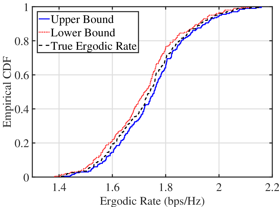
Proposition 1 : The ergodic rate at device is $k$ bounded as $\hat{r}_{k}^{\circ}(\rho_{k},\mathbf{\Theta})\leq\overline{r}_{k}(\rho_{k},\mathbf{\Theta})\triangleq\mathbb{E}_{\mathbf{\hat{H}},\bm{\phi}_{k}}[\log_{2}(1+\textrm{$\Gamma$}_{k}(\rho_{k},\mathbf{F},\hat{\bm{h}}_{k},\bm{\phi}_{k}))]$, and $\hat{r}_{k}^{\circ}(\rho_{k},\mathbf{\Theta})\geq$

Here the lower bound follows from the properties of variance and the Cauchy–Schwarz inequality. From Proposition 1, optimizing the lower and upper bound provide the same optimal solution. Moreover, as verified in Fig. 2, we find that both bounds are tight. Therefore, we optimize the lower (upper) bound of the ergodic rate at each device as it is more tractable for optimization.

The average harvested power conditioned on imperfect CSI $\hat{\bm{h}}_{k}$ of device $k$ follows a non-linear function [8] and can be expressed as $\overline{e}_{k}^{\circ}(\rho_{k},\mathbf{F}|\hat{\bm{h}}_{k})=\mathbb{E}_{\bm{\phi}{}_{k}}[\hat{e}_{k}^{\circ}(\rho_{k},\mathbf{F}|\hat{\bm{h}}_{k},\bm{\phi}_{k})],$ where

where $S_{k}$ is a constant denoting the maximum harvested power at the $k$th device, $\Psi_{k}\triangleq\frac{S_{k}}{1+\mathrm{exp}(-a_{k}(P_{k}-b_{k}))}$, $\Omega_{k}\triangleq\frac{1}{1+\mathrm{exp}(a_{k}b_{k})}$, and parameter $a_{k}$ and $b_{k}$ are constants related to the circuit specifications, and $P_{k}\triangleq(1-\rho_{k})(\sum_{m=1}^{K}|(\hat{\bm{h}}_{k}+\bm{\phi}_{k})^{H}\bm{f}_{m}|^{2}+\sigma_{k}^{2})$ is the input RF power for the $k$th device. Then, the average harvested power of user $k$ is defined as $\overline{e}_{k}(\rho_{k},\mathbf{\Theta})=\mathbb{E}_{\mathbf{\hat{H}}}[\overline{e}_{k}^{\circ}(\rho_{k},\mathbf{F}\left(\mathbf{\hat{H}}\right)|\hat{\bm{h}}_{k})]$.

We are interested in a mixed-timescale joint optimization of digital beamformer and power splitter to balance the average ergodic rate and the average harvested power. This can be formulated as the following network utility maximization problem:

where $\overline{\eta}_{k}(\rho_{k},\mathbf{\Theta})\triangleq\overline{r}_{k}(\rho_{k},\mathbf{\Theta})+\gamma_{k}\overline{e}_{k}(\rho_{k},\mathbf{\Theta})$ with the corresponding weight $\gamma_{k}$ is a weighted sum of the average ergodic rate and the harvested power, $\Phi\triangleq\{\bm{\rho}=[\rho_{1},\cdots,\rho_{K}]^{T}|\rho_{k}\in(0,1],\forall k\}$ is the feasible set of power splitters. The utility function $g\left(\overline{\eta}_{k}\right)$ is a continuously differentiable and concave function of $\overline{\eta}_{k}$. Moreover, $g\left(\overline{\eta}_{k}\right)$ is non-decreasing w.r.t. $\overline{\eta}_{k},$ and its derivative $\nabla_{\overline{\eta}_{k}}g\left(\overline{\eta}_{k}\right)$ is Lipschitz continuous.

In this section, we propose a MO-SSCA algorithm to solve the mixed-timescale stochastic non-convex optimization problem $\mathcal{P}$, and summarize it in Algorithm 1. In MO-SSCA, we focus on a coherence time of channel statistics, where the time is divided into $T_{f}$ frames and each frame consists of $T_{s}$ time slots. At beginning, the BS initializes the MO-SSCA algorithm with power splitter $\bm{\rho}^{0}$ and a weight vector $\bm{v}^{0}$. In subsequent, $\bm{\rho}$ and $\bm{v}$ are updated once at the end of each frame. Then we elaborate the implementation details of the iteration of the MO-SSCA algorithm at the $t$-th frame.

We consider a single-cell of radius $100$ m, where BS is equipped with $64$ antennas. There are 12 devices randomly distributed in the cell. We adopt a geometric channel model with a half-wavelength space ULA for simulations [7]. The channel between BS and device $k$ is given by $\boldsymbol{h}_{k}=\sum_{i=1}^{N_{p}}\varepsilon_{k,i}\boldsymbol{\textrm{a}}\left(\varphi_{k,i}\right)$, where $\boldsymbol{\textrm{a}}\left(\varphi\right)$ is the array response vector, $\varphi_{k,i}$’s are Laplacian distributed with an angular spread $\sigma_{\textrm{AS}}=10$, $\varepsilon_{k,i}\sim\mathcal{CN}\left(0,\sigma_{k,i}^{2}\right)$, $\sigma_{k,i}^{2}$ are randomly generated from an exponential distribution and normalized such that $\sum_{i=1}^{N_{p}}\sigma_{k,i}^{2}=G_{n,k}$, $G_{k}$ is the average channel gain determined by the pathloss model $30.6+36.7\log 10\left(\textrm{ds}_{k}\right)$ [15], and $\textrm{ds}_{k}$ is the distance between BS and device $k$ in meters. We consider $N_{p}=6$ channel paths for each device. The transmit power budget for BS is $P_{\mathrm{max}}=10$ dBm. We set $N=200$, $S_{k}=24$ mW, $a_{k}=150$, $b_{k}=0.014$, $\gamma_{k}=10$, $\omega_{k}^{2}=-40$ dB, $\sigma_{k}^{2}=-60$ dBm and $\delta_{k}^{2}=-50$ dBm. There are $T_{s}=10$ time slots in each frame and the slot size is 2 ms. The coherence interval $T=400$, which corresponds to a coherence time of 2 ms and a coherence bandwidth of 200 kHz [16]. The coherence time for the channel statistics is assumed to be 10 s. We use the average sum utility $g\left(\hat{\bm{\eta}}\right)=\sum_{k=1}^{K}\hat{\eta}_{k}$ as an example to illustrate the advantages of the proposed scheme. Two schemes are included as baselines: 1) maximum ratio transmission (MRT) scheme, which is obtained by fixing the MRT beamformer [3]; 2) zero-forcing (ZF) scheme, which is obtained by fixing the ZF beamformer [5]. The power splitters of both MRT and ZF scheme are obtained by the long-term optimization.

In Fig 3, we plot the utility performance versus the signal-to-noise ratio (SNR). We can see that as the SNR increases, the average sum utility of all schemes increases gradually. It is observed that the average sum utility achieved by the proposed MJBP scheme is higher than that achieved by the other schemes for moderate and large SNR. This indicates that the proposed MJBP scheme can better mitigate the multi-device interference to achieve better tradeoff between the average ergodic rate and the average harvested power, which is further validated in Fig 3.

In Fig 4, we plot the utility performance versus the number of devices $K$. We observe that the proposed MJBP scheme achieves significant gain over MRT scheme and ZF scheme, which demonstrates the importance of mixed-timescale joint optimization. Moreover, as the number of devices $K$ increases, the performance gap between the proposed MJBP scheme and other competing schemes becomes larger.

In Fig 4, we plot the utility performance versus the number of antennas at BS. It shows that the performance of all these schemes is monotonically increasing with the number of antennas. Again, it is seen that the proposed MJBP scheme outperforms all the other schemes for all $M$ regime.

In this letter, we considered mixed-timescale joint beamforming and power splitting (MJBP) scheme in the downlink transmission of massive MIMO aided SWIPT IoT network to maximize the network utility under the power budget constraint. We proposed a MO-SSCA algorithm to find stationary solutions of the mixed-timescale non-convex stochastic optimization problem. Simulations verify that the proposed MJBP scheme achieves significant gain over existing schemes.

References

- [1] M. Swan, “Sensor mania! the Internet of things, wearable computing, objective metrics, and the quantified self 2.0,” J. Sens. Actuator Netw, vol. 1, no. 3, pp. 217–253, 2012.
- [2] R. Zhang and C. K. HO, “MIMO broadcasting for simultaneous wireless information and power transfer,” IEEE Trans. Wireless Commun., vol. 12, no. 5, pp. 1989–2001, May 2013.
- [3] Q. Shi, L. Liu, W. Xu, and R. Zhang, “Joint transmit beamforming and receive power splitting for MISO SWIPT systems,” IEEE Trans. Wireless Commun., vol. 13, no. 6, pp. 3269–3280, Apr 2014.
- [4] Q. Shi, W. Xu, T. Chang, Y. Wang, and E. Song, “Joint beamforming and power splitting for MISO interference channel with SWIPT: An SOCP relaxation and decentralized algorithm,” IEEE Trans. Signal Process., vol. 62, no. 23, pp. 6194–6208, Dec 2014.
- [5] G. Dong, H. Zhang, and D. Yuan, “Optimal downlink transmission in Massive MIMO enabled SWIPT systems with zero-forcing precoding,” IEEE Global Commun. Conf., Dec 2014.
- [6] G. Caire, “On the ergodic rate lower bounds with applications to masssive MIMO,” IEEE Trans. Wireless Commun., vol. 17, no. 5, pp. 3258–3268, May 2018.
- [7] A. Liu, X. Chen, W. Yu, V. Lau, and M. Zhao, “Two-timescale hybrid compression and forward for massive MIMO aided C-RAN,” IEEE Trans. Signal Process., vol. 67, no. 9, pp. 2484–2498, Mar 2019.
- [8] E. Boshkovska, D. Ng, N. Zlatanov, and R. Schober, “Practical non-linear energy harvesting model and resource allocation for SWIPT systems,” IEEE Commun. Lett., vol. 19, no. 12, pp. 2082–2085, Dec. 2015.
- [9] A. Shapiro, D. Dentcheva, and A. Ruszczynski, Lecture on stochastic programming: modeling and theory. SIAM, 2009.
- [10] K. Shen and W. Yu, “Fractional programming for communication systems – Part II: Uplink scheduling via matching,” IEEE Trans. Signal Process., vol. 66, no. 10, pp. 2631–2644, Mar 2018.
- [11] M. W. Jacobson and J. A. Fessler, “An expanded theoretical treatment of iteration-dependent majorize-minimize algorithms,” IEEE Transactions on Image Processing, vol. 16, no. 10, pp. 2411–2422, Oct 2007.
- [12] “CVX Research, Inc. CVX: Matlab software for disciplined convex programming, version 2.0 beta.” Sep, 2012. [Online]. Available: http://cvxr.com/cvx.
- [13] K. Shen, W. Yu, L. Zhao, and D. P. Palomar, “Optimal of MIMO device-to-device networks via matrix fractional programming: A minorization-maximization approach,” arXiv.org:1808.05678, 2019.
- [14] H. Sun and H. Xu, “A note on uniform exponential convergence of sample average approximation of random functions,” J. Math. Anal. Appl, pp. 698–708, 2012.
- [15] Technical Specification Group Radio Access Network; Further Advancements for E-UTRA Physical Layer Aspects, 3GPP TR 36.814. [Online]. Available: http://www.3gpp.org
- [16] T. Marzetta, E. G. Larsson, H. Yang, and H. Ngo, Fundamentals of Massive MIMO. Cambridge, U.K.: Cambridge University Press, 2016.