A Fast Integral Equation Method for the Two-Dimensional Navier-Stokes Equations
Abstract
The integral equation approach to partial differential equations (PDEs) provides significant advantages in the numerical solution of the incompressible Navier-Stokes equations. In particular, the divergence-free condition and boundary conditions are handled naturally, and the ill-conditioning caused by high order terms in the PDE is preconditioned analytically. Despite these advantages, the adoption of integral equation methods has been slow due to a number of difficulties in their implementation. This work describes a complete integral equation-based flow solver that builds on recently developed methods for singular quadrature and the solution of PDEs on complex domains, in combination with several more well-established numerical methods. We apply this solver to flow problems on a number of geometries, both simple and challenging, studying its convergence properties and computational performance. This serves as a demonstration that it is now relatively straightforward to develop a robust, efficient, and flexible Navier-Stokes solver, using integral equation methods.
Keywords:
Navier-Stokes equations , Integral equations , Function extension , Quadrature1 Introduction
Fast integral equation methods (FIEMs) - techniques based on integral equations coupled with associated fast algorithms for the integral operators such as the Fast Multipole Method (FMM) [30] or fast direct solvers [46] - have become the tool of choice for solving the linear, elliptic boundary value problems associated with the Laplace and Helmholtz equations, the equations of elasticity, the Stokes equation, and other classical elliptic equations in mathematical physics. For these boundary value problems, FIEMs have been a game changer: superior stability and accuracy, efficiency through dimension reduction and acceleration, and ease of adaptivity are a few of the more significant advantages.
While nonlinear equations are not directly amenable to solution via integral equation methods, for some equations a suitable temporal discretization and/or linearization gives rise to a sequence of “building-block” partial differential equations (PDEs) of the form of the classic equations mentioned above. These can then be targeted with suitably-chosen FIEMs. The focus of this paper is to discuss a FIEM-based solver for the two-dimensional incompressible Navier-Stokes equations (INSE),
| (1) |
on a general bounded domain and satisfying the no-slip boundary conditions. In this context, the basic idea is as follows. Applying a semi-implicit temporal discretization to the momentum equation in (1) gives rise to a sequence of modified biharmonic (in the stream function formulation, c.f. [39]) or modified Stokes equations,
| (2) | ||||||
where , is the time step, and with being updated at each time step. This is the so-called Rothe’s method or Method of Lines Transpose. It is (2), then, that are recast by representing the solution as the sum of suitably chosen layer and volume potentials. This representation will satisfy the incompressibility constraint by construction, thereby eliminating the need for artificial boundary conditions associated with projection and other methods based on direct discretization of the Navier-Stokes equations. The focus of this paper, then, is to present a FIEM for (2) in general, two-dimensional bounded domains and to examine their performance for a range of .
This general approach was examined in [28] for the special case of flow inside a circular cylinder. It was demonstrated in this paper that FIEMs have a great deal of potential computing solutions for Reynolds number up to with both high spatial and temporal accuracy. Despite inspiring some other integral equation-based solvers for the INSE [14], this work has yet to be fully realized in general 2-D or 3-D domains. As outlined in [42], there have been two critical stumbling blocks in achieving this goal. The first is how to evaluate the layer potentials close to the boundary where the kernels become nearly singular. There are many high-order quadrature methods that are well-suited for discretizing the integral operators and evaluating potentials away from the boundary [32], but these break down when the target becomes close to source points on the boundary. The second stumbling block is how to solve inhomogenous equations on general domains. A potential theoretic approach expresses the particular solution as a volume potential: a convolution of the fundamental solution with the right hand side of the equation. Unfortunately, available fast methods for evaluating layer potentials are generally in the form of “box codes" such as [18] or the FFT. These require knowing the source data throughout a square or cube. In order for these box codes to be effective, this data must be of sufficient regularity throughout the box. For a boundary value problem on a general domain, this then requires extending the right-hand side with the required regularity throughout the bounding box.
Recently, significant progress has been made on both the quadrature and function extension fronts. Developing specialized quadrature that can be used to evaluate potentials arbitrarily close to the boundary and which employs the governing hierarchical acceleration strategy has been an area of active research. One approach is “Quadrature By Expansion”, or QBX [10, 41], which uses local expansions with centres close to the boundary. QBX has the advantage that it can be extended to three dimensions but it can be challenging to integrate it effectively within an FMM. Another approach is an explicit kernel-split, panel-based Nyström method outlined in [34, 36]. Here, the kernel is split into its smooth and regular parts, with the smooth parts being evaluated using a composite n-point Gaussian quadrature scheme, and the singular parts using specialized quadrature based on product integration. In our case, the kernel-splitting of the Stokes kernel is considerably more complex with an additional complication that the underlying kernels require more spatial resolution for larger values of (corresponding to large or small time steps). A straightforward implementation of [34] shows a breakdown in accuracy which requires careful local refinement to alleviate this [5]. The result is a quadrature scheme which is robust for arbitrary target points and values of .
Two approaches have been investigated recently which extend functions throughout a bounding box in which the geometry of the problem is embedded. One approach uses extension via layer potentials [7, 9]. The layer potential is determined by enforcing continuity across the boundary of the domain through solving an integral equation, and it is then used to construct the function extension in the complement of the domain. Requiring a higher degree of continuity means the integral equation is based on solving a higher-order partial differential equation and this can get prohibitively complex. A second approach, which is the approach we take here, is to smoothly extend the right-hand-side of (4) via extrapolation using radial basis functions [23, 24]. This method is called Partition of Unity eXtension, or PUX. It is then simple to convolve this extended function with the periodic Green’s function for these equations using a fast Fourier transform (FFT) and the solution may be evaluated on the boundary rapidly with a non-uniform FFT [11].
The methods we propose in this paper consist of coupling together existing and custom-developed state-of-the-art tools for constructing and evaluating the layer and volume potentials. The key elements of the overall approach and the road map to where these elements are discussed in this paper are summarized below:
- 1.
Using PUX, the function is extended onto a uniform grid discretizing the bounding box. The volume potential is evaluated on this grid via an FFT and evaluated on via a non-uniform FFT. This is discussed in section 3.1.
- 2.
To the volume potential, layer potentials are added which ensure the solution satisfies the no-slip boundary conditions . This involves solving a system of Fredholm integral equations of the second kind for the homogenous modified Stokes equations (see section 2.2). After applying quadrature (see section 4), the resulting linear system is dense and of the form of , where represents the time step and is has low-rank structures. Since the boundary is fixed, the system matrix does not change throughout time. We use a fast direct method [25, 45] which exploits the low-rank off-diagonal blocks to invert the system matrix as a precomputation. This inverse can be applied to the updated vector at each time step at a fraction of the time. All computations are linear in computational time. This is discussed in section 3.2.2.
- 3.
Given the density of the layer potentials, , from the previous step, and are evaluated at all regular grid points in . Special-purpose quadrature is used when evaluating the layer potentials close to the source terms [5] (see section 4). These point-to-point interactions are accelerated by an FMM [30] based on the separation of variables formulae derived in [8], which are stable for all values of (section 3.2.1). These values are used to construct a new right hand side in .
- 4.
The above steps are repeated for the next time step. The solution is advanced using a semi-implicit spectral deferred correction method [47]. This is discussed in section 3.3.
The result is a Navier-Stokes solver which has linear or near-linear scaling in computational time at each time step, specifically the computational cost is , where and denote the number of discretization nodes in the domain and on the boundary, respectively. We show in section 5.5 that the stability requirement is . The numerical experiments, which we present in section 5, indicate that our methods are well suited for problems with moderate values of the Reynolds number.
Our approach could be described as an embedded boundary approach, which is a popular approach for methods based on direct discretization of the PDE, such as the Immersed Boundary (IB) method of Peskin [50]. Here, the effect of the boundary is smeared to neighboring grid cells (including the cut cells) by using approximations to the Dirac function. The original IB framework was limited to low order accuracy; recently, Stein et al. [56] presented a higher-order IB approach based on envisioning a smooth extension of the solution outside of the original domain. The ideas behind the resulting method, IB Smooth Extension (IBSE), bear some resemblance to the present work but are based on introducing new unknowns for the solution outside of the domain as opposed to extending the known inhomogeneity, as we describe below. Further references for embedded boundary methods in the PDE literature can be found in [56].
There has been recent work on time-dependent integral equation methods for the unsteady Stokes equations [27, 31, 59], which could form the basis of a FIEM-based Navier-Stokes solver quite different from the one presented here. These methods are still in the early stages of development, but are nevertheless promising. In particular, their formulation allows for a natural treatment of moving boundaries, and would likely have advantages in terms of stability.
The remainder of this paper is organized as follows. Section 2 introduces the underlying mathematical formulation. Section 3 outlines the framework of numerical methods. Section 4 gives a detailed description of the quadrature used for singular and nearly singular integrals. Section 5 reports on results from numerical experiments. Finally, concluding remarks are provided in section 6, while supplementary material is available in appendices A, B and C.
2 Formulation
Many numerical approaches to solving the Navier-Stokes equations begin by performing a discretization of the equations in time. Because it is simpler to handle the nonlinear term explicitly but less restrictive to handle the stiff diffusion term implicitly, it is common to use an implicit-explicit (IMEX) method [6]. Using the first-order IMEX-Euler rule results in the time-independent elliptic PDE
| (3) | ||||||
The higher-order IMEX rules result in qualitatively similar elliptic PDEs. Further, the spectral deferred corrections (SDC) method [19] can be used to combine many low order IMEX steps into a high order scheme for advection-diffusion problems [47], which will be the approach of this paper.
It is in the solution of the elliptic PDE (3), called the modified Stokes equations11 1 These equations may also be referred to as the linearized unsteady Stokes equations [51], or the Brinkman equations [16]. where the PDE discretization and integral equation methods diverge. Because the equation is linear in the unknowns , the solution of (3) can be split into a particular and a homogeneous problem,
| (4) | ||||||
and
| (5) | ||||||
where
| (6) |
The forced PDE (4) has no boundary conditions, so that a candidate particular solution may be computed by convolving the right-hand-side of (4) with a free-space or periodic Green’s function — in particular, a Green’s function which is independent of the domain and analytically known. Regardless of the particular solution chosen, the homogeneous equation (5) is specified so that the composite solution,
| (7) | ||||
| (8) |
satisfies the original problem (3). For this reason, the homogeneous solution is sometimes referred to as a boundary correction.
In an integral equation method, the homogeneous solution is generally represented by the convolution of an unknown density defined on the boundary, , with an integral kernel given in terms of the equivalent of a charge or a dipole of the equations (5), which a priori satisfies the divergence-free condition and the homogeneous equations inside the domain. For a well-chosen representation, the enforcement of the boundary conditions gives a well-conditioned equation for the density on the boundary. Once this boundary integral equation is solved, the homogeneous solution may be evaluated at any point in the domain by convolution.
The central equation of our method is the inhomogeneous modified Stokes equations with Dirichlet boundary conditions,
| (9) | ||||||
This stationary problem is the result of a semi-implicit discretization of the Navier-Stokes equations (3). Because of the divergence-free condition, these equations, like the Navier-Stokes equations, imply a compatibility condition on , namely
| (10) |
In analogy with the regular Stokes equations, we call the free-space Green’s function of these equations the modified stokeslet tensor, or simply the stokeslet. It is defined as
| (11) |
where
| (12) |
is the free-space Green’s function of the modified biharmonic equation, i.e. [39]. The corresponding pressure vector and stress tensor (which we will refer to as the stresslet) are defined as
| (13) | ||||
| (14) |
Note that if is the field induced by a stokeslet with charge , then the stress tensor for that field, , is given by
| (15) |
Closed-form expressions for , , and are derived in appendix B.
Our solution strategy for the equations (9) is based on two fundamental principles, which are typical of integral equation methods. The first principle is the use of potential theory, in which the solution is represented using convolutions with Green’s functions of the equations. By construction, this guarantees that the divergence-free condition is satisfied, in contrast with methods based on direct discretization of the PDE. The second principle is the use of a composite solution, which is formed by the solutions to the particular problem (4) and the homogeneous problem (5). This split allows us to use numerical methods that are fast and geometrically flexible, as we shall see in section 3. In the remainder of this section, we describe in detail how the Green’s functions are used to solve the particular and homogeneous problems.
2.1 Particular solution
From a mathematical point of view, the most straightforward solution to the particular problem (4) is the volume potential,
| (16) |
which solves (4) using free-space boundary conditions. This is however not practical, as evaluating the integral (16) accurately over a complex domain would present a significant numerical challenge. Instead, we shall for the moment assume that is embedded in a square domain (see fig. 1), and that there exists a compactly supported function that is a q-continuous extension of out into ,
| (17) | ||||
| (18) | ||||
| (19) |
We will return to the computation of the extension in section 3.1.1. Having lets us compute as the solution to the extended particular problem,
| (20) | ||||||
Note that the solution to the extended particular problem (20) also satisfies the original particular problem (4). Now, since is a simple domain (a box), it would be straightforward to compute the particular solution as the volume potential over with the extended function . Alternatively, and this is the path we will follow, we can compute it using a Fourier series. This amounts to solving (20) using periodic boundary conditions, which we can do since is compactly supported, and therefore also periodic. Let
| (21) |
Replacement into (20) and matching of coefficients gives the linear system of equations
| (22) | ||||
| (23) |
with solution
| (24) |
To rephrase the above, given a smooth extension of with Fourier coefficients , a solution of the particular equation, eq. 4, is given by the convolution
| (25) |
where is the Fourier multiplier corresponding to the periodic stokeslet, i.e.
| (26) |
We also need the gradient of the solution, in order to compute the right hand side of the next time step (6). This is straightforward to compute using Fourier differentiation,
| (27) |
This solution procedure has some nice properties. First, once the extension is available, computing the particular solution does not require that a linear system be solved; instead, the computation is based on evaluating a formula for the solution. Further, for smaller values of , the multiplier is strongly smoothing, i.e. it decreases the magnitude of higher Fourier modes. This property is both consistent with the physics and stabilizing from a numerical point of view. Unfortunately, this smoothing property is reduced for large values of , corresponding to high Reynolds number flow.
2.2 Homogeneous solution
The solution to the homogeneous problem (5) can be represented by a double layer potential, which we denote by
| (28) |
For a given double layer density defined on , the potential is defined as the boundary integral
| (29) |
where the double layer kernel, , is defined using the stresslet (14) and the surface unit normal pointing into ,
| (30) |
By construction, this layer potential is divergence-free and satisfies the homogeneous modified Stokes equation in .
We will now briefly describe how a double layer potential is used to solve the homogeneous Dirichlet problem. Much of the following depends on a number of technical results concerning the double layer potential which can be found in the literature [40, 52, 14] and are included in Appendix A for convenience. In contrast with the Stokes equation, we note that all of the following holds without modification for multiply-connected . The appropriate density is determined by enforcing the Dirichlet boundary condition in the limit . Using the jump conditions for modified Stokes layer potentials (see Lemma 2 in appendix A), we obtain a second-kind integral equation in ,
| (31) |
This integral equation has a null space of rank 1 (see Lemma 3 in appendix A), so in order to have a unique solution we add the term
| (32) |
which is sometimes referred to as a nullspace correction. Then, the homogeneous solution is given by a double layer potential (28), with the density satisfying
| (33) |
The new equation, eq. 33, is invertible for any right hand side and the term is zero provided that the right hand side satisfies the condition (see Lemma 4 in appendix A)
3 Numerical methods
This section gives a complete outline of the numerical methods used. Quadrature will only be briefly discussed in this section, and more thoroughly covered in section 4.
3.1 Evaluating the particular solution
3.1.1 Smooth function extensions
In order compute the particular solution using the Fourier method of section 2.1, we need an extended forcing function with a high order of regularity. To compute such a function extension, we use the method known as PUX, for Partition of Unity eXtension, introduced in [23]. The method is based on overlapping circular partitions with their centers distributed along the boundary . Inside each partition radial basis functions (RBFs) are defined, which interpolate at each point of the partition inside , giving a local extrapolation of to the other points in the partition. These exterior values in adjacent partitions, which can be multiply-defined due to the overlap, are then blended using a high-order partition of unity (POU) function, forming a function extension with high regularity. Finally, the extension is given compact support by blending it with a second layer of “zero partitions”, located just outside .
The current version of PUX is limited to a uniform grid in , and we will use a uniform grid for that reason. Given a grid and a boundary, [23] provides heuristics for determining the parameters of the method; the only free parameters are the RBF shape parameter (which is set to 2 throughout) and the partition radius . The accuracy largely depends on the number of grid points spanned by ; the more grid points spanned, the better the decay of the extension can be resolved, up to a limit. The range of points spanned by is typically between 20 and 50.
3.1.2 Evaluating the volume potential
After applying the PUX algorithm, we have the values of the smooth extension on a uniform grid in . It is then straightforward to compute the particular solution (25) in a fast way, using fast Fourier transforms (FFTs). First, two FFTs give us the Fourier coefficients . We can then compute the solution using two inverse FFTs for the volume grid, and two non-uniform FFTs of type 2 [11] for the discretization points on . The gradient (27) is then computed using four additional inverse FFTs. Since the gradient is only needed on the volume grid, it does not require any non-uniform FFTs.
For a discretization with uniform points in B, and nonuniform points on , the computational cost is . The method has spectral accuracy if and its extension are smooth. If they are not smooth, the order of accuracy is related to the regularity of the extended function.
3.2 Computing the homogeneous correction
In order to solve the integral equation (33), we first need to discretize the boundary using a suitable quadrature. For this, we use a composite Gauss-Legendre quadrature, wherein is subdivided into panels of equal arclength,
| (35) |
each of which is discretized using an -point Gauss-Legendre quadrature (we use throughout this work). If we let be the mapping from the standard interval to the panel , then
| (36) |
Here are the standard Gauss-Legendre nodes and weights on . For convenience, we now combine the double summation over and into a single index that runs to , and let and . This gives us a set of nodes and weights for approximating integrals over . Given the double layer density at the nodes, we can then approximate the double layer potential (29) anywhere in as
| (37) |
As long as and are properly resolved, this quadrature will be accurate for target points that are well-separated from . However, straight Gauss-Legendre quadrature will not be accurate for target points close to, or on, the boundary . This is due to the singularities in the stresslet (14). We will discuss specialized quadrature methods for such cases in section 4. For now, we write , with the understanding that these weights are only dependent on at the finite number of boundary points located close to .
We approximate the integral equation using the quadrature (37), including specialized quadrature weights where needed, and enforce it at the quadrature nodes (this is known as the Nyström method). This gives us the dense linear system
| (38) |
As this is a second-kind integral equation, it can be solved iteratively using GMRES [54] in a number of a iterations that is bounded as grows. We can then evaluate the homogeneous solution on the domain grid using (37). If done naively, both of these steps have quadratic costs, which is infeasible for large systems. To get around this, we make use of fast hierarchical methods, described in sections 3.2.1 and 3.2.2.
3.2.1 Fast summation
Let denote the number of grid points which lie inside (in Figure 1 this is the number of black dots). A naive evaluation of eq. 37 at each of these points would require operations. Using the fast multipole method (FMM) [30], it is possible to reduce this computational cost to , by taking advantage of special structure in the sum. In this section, we describe some components of an FMM based on the special functions defined in [8].
Nomenclature
In analogy with physics, we refer to a Green’s function as a charge located at , a derivative of as a dipole, a second derivative of as a quadrupole, and a third derivative of as an octopole. By the definition of the double layer potential, the quadrature formula eq. 37 is a sum of dipoles and octopoles for the modified biharmonic equation which are located along . These charges and higher moments are referred to as sources and the points at which we would like to evaluate the field are called targets.
Well-separated interactions
Suppose you can define two boxes around a set of points such that they share the same center, the larger box has three times the side length, and the smaller box contains all of the points. Points located outside of the larger box are said to be well-separated from the original points, see fig. 2a for an illustration. An important property of well-separated interactions is that the field induced by a set of source points is smooth from the perspective of well-separated points and can be approximated accurately using relatively few terms in a separation of variables expansion, independent of the number of source points.
Separation-of-variables representations
Because the field induced by the sources satisfies the modified biharmonic equation, standard separation-of-variables techniques apply. Let and denote the modified Bessel functions of the first and second kind, respectively. Classically, a field which satisfies the modified biharmonic equation can be represented in the exterior of the disc as a series in , , and and in the interior of a disc as a series in and , where is the radial part of polar coordinates centered in the disc. Using these classical functions directly leads to catastrophic cancellation when is small. Following [8], we define the functions and via
| (39) | ||||
| (40) |
and
| (41) |
Consider a disc centered at a point and let denote the polar coordinates of a point . Then, the field, , induced by a collection of sources inside the disc can be represented by
| (42) |
which we will refer to as a multipole expansion, and the field, , induced by a collection of sources outside the disc can be represented by
| (43) |
which we will refer to as a local expansion. These expansions can be manipulated stably. In particular, [8] provides stable formulas for shifting the centers of the expansions and converting a multipole expansion about one center into a local expansion about another. When evaluating the expansions for a collection of sources which are well separated from the targets, the standard decay rates in [29, 18] apply, so that truncating the sums in eqs. 42 and 43 to order , i.e. retaining only the terms with , is sufficient to achieve 12 digits of accuracy.
Tree structure
To deal with arbitrary collections of sources and targets, as opposed to well-separated ones, the source and target points are arranged in a hierarchical quad-tree structure in the FMM. Starting from a root box containing all sources and targets, the tree nodes (boxes) are subdivided equally into four quadrants, which are its children nodes, until they have at most a prescribed total number of source and target points inside. Typically, the maximum number of points is set to the order of the expansions used to represent the well-separated interactions. Many FMM algorithms are written for arbitrary quad-trees; for simplicity, we add a level-restriction to the tree: all adjacent leaf boxes should be within one level of refinement.
The FMM gains its efficiency by organizing the interactions between sources and targets hierarchically in this tree so that most interactions are treated as well-separated. This is done using a number of standard techniques, see [29, 30] for a reference. Below, we only describe how multipole and local expansions are formed on leaf boxes, as the other techniques are a straightforward application of the translation formulas in [8].
Form multipole and form local
Consider the sources contained within a leaf box. Note that a charge can be represented perfectly as a 0-term expansion about its own center because , with . Because we are concerned with up to octopole moments of the Green’s function, we derive expressions for first, second, and third order directional derivatives of in the multipole basis . As in appendix B, we make use of the standard suffix notation and set .
The following identities are straightforward to derive. We have
| (44) | ||||
| (45) | ||||
| (46) | ||||
From the recurrence and derivative relations for modified Bessel functions [48, S10.29], we obtain
| (48) | ||||
| (49) | ||||
| (50) | ||||
| (51) | ||||
| (52) |
To derive the separation of variables form of the directional derivatives, we identify the point with . In the following, we switch freely between identifying vectors by their suffix and complex valued notations. Let be vectors and denote their complex valued counterpart. Then,
| (53) |
so that
| (54) |
Similarly, we have that
| (55) | ||||
| (56) |
so that
| (57) |
Finally, we have that
| (58) | ||||
| (59) |
so that
| (60) |
Remark 1.
Note that the terms always have a coefficient which is the complex conjugate of the terms. This is used by the fast multipole method to reduce the storage for expansions and to reduce the computational cost of translating expansions.
Once the exact separation of variables representation for a charge or higher order moment of is obtained from the formulas above, one can simply use the translation formulas for multipole expansions to shift each of the per-source expansions to the center of the leaf box. The cost of this operation depends on the number of sources, but is only performed on leaf boxes. Similarly, the per-source expansions can be translated, transformed, and added to the local expansion in any box for which the sources are well-separated.
3.2.2 Fast direct solver
Let be the matrix corresponding to the discretized boundary integral equation, eq. 38, so that
| (61) |
with and . Naïve inversion of this matrix would require floating point operations. However, the complexity of inversion can be reduced to by taking advantage of structure within the matrix.
The ability to use a truncated multipole expansion to represent well-separated interactions to high precision, as in the previous section, implies that sub-matrices of for which the row points are well-separated from the column points are of low numerical rank (and likewise when the column points are well-separated from the row points). Because of these low rank structures in the matrix, there is an ordering of the indices for which the matrix is hierarchically block separable (HBS), as in [25, 45]. For such matrices, it is possible to efficiently compute a compressed representation of the matrix in operations and using storage. Then, a representation of the inverse can also be computed and applied in operations based on that compressed representation. Such methods combine matrix compression [17] with a variant of the Sherman-Woodbury-Morrison formula and take advantage of hierarchical features of the matrix, as in the FMM. See [25, 45] for more details.
A common feature of fast direct solvers is that there is a relatively large upfront cost in forming the representation of the inverse while the cost of the subsequent linear system solves for any given right hand side is orders of magnitude smaller. This is well-suited to the numerical examples in this paper, where we have a fixed boundary discretization and use a fixed time step length. We only pay the upfront cost once and use the same representation of the inverse for fast system solves at each step in the simulation.
Remark 2.
Technically, the scaling of the HBS method depends on a more subtle aspect of the low-rank structure of the matrix. Because the boundary points are contained to a one dimensional curve, even the interactions between adjacent sections of the curve are of relatively low rank. This is illustrated in fig. 2b for two adjacent sections of the boundary, one gray and one black. Observe that the points on the gray portion of curve are approximately well-separated from each set of points between the dotted separators on the black portion of the curve.
3.3 Time stepping
The integral equation approach that we have outlined so far is based on a first order IMEX discretization of the Navier-Stokes equations (3). In order to increase the temporal order of accuracy, we use the semi-implicit spectral deferred corrections (SISDC) method [47]. Consider an autonomous initial value problem of the form
| (62) | ||||
| (63) |
where is a stiff part that needs implicit treatment, and is a nonlinear term that would be impractical to treat implicitly. The method is based on dividing a time interval , , into subintervals by choosing points such that , with . A first approximation of on , denoted , is computed at the substeps using a first order IMEX discretization,
| (64) | ||||
| (65) |
Then, a sequence of increasingly accurate approximations are computed at the nodes using the correction equation
| (66) | ||||
all initialized to . The computation of is in this context considered one application of the correction equation. The term is a quadrature approximation of the integral
| (67) |
The quadrature is precomputed, so that computing the integral requires only a small matrix-vector multiplication, as in
| (68) |
The weights are chosen so that they integrate the interpolating polynomial through the points, which gives an error in each quadrature. In [47] the points are chosen to be the nodes of Gauss-Lobatto quadrature. This choice ensures that the polynomial interpolation is well-conditioned for high order schemes, while conveniently including nodes at the beginning and end of the interval.
Each application of the correction equation increases the local order of accuracy by one, so that if , then after corrections we have
| (69) |
A SISDC time stepping method with global order of accuracy therefore requires substeps and applications of the correction equation. Taking into account the steps taken to compute the first approximation (64), the total number of implicit linear system solves needed to take one step of length is then , resulting in the final approximation .
In our case, the equation of interest is the momentum equation of the Navier-Stokes equations (1). We split the equation into implicit and explicit parts as before, setting
| (70) | ||||
| (71) |
Our scheme for the modified Stokes equation relies on precomputing a solver and quadrature rules for a specific , which in this context is a function of the substep length. To reduce the precomputation time and storage, it is therefore preferable for us to use substeps that are of equal length . This coincides with the points used by [47] for (where ) and (since 3-point Gauss-Lobatto is equidistant). For moderate values of , equispaced substeps could still be feasible, though at some level of the ill-conditioning of polynomial interpolation on equispaced nodes would make itself known.
Assuming a constant substep length of , the first approximation is computed by using our composite scheme to solve the modified Stokes equation (9),
| (72) |
with the forcing function from the original IMEX scheme (3),
| (73) |
To apply the correction equation, we solve the same PDE,
| (74) |
this time with the right hand side
| (75) |
and the quadrature term
| (76) |
For the first order IMEX scheme, we need to compute the solution and its gradient on the grid at every substep, and we also need them at the initial time to start the simulation. In addition to that, the SISDC scheme also requires the quantity at every substep, and at the initial time. At a substep we can compute this quantity without actually having to compute and separately, simply by recovering it from the equation solved to compute the solution at that substep,
| (77) |
For the initial time, this quantity is not available. Note that, when added to the right hand side, any irrotational term (which is the gradient of a scalar function) has no effect on the computed velocity field. Therefore, we only require the value of be supplied at the initial time and use instead of in correction equations for the first interval.
Remark 3.
The fact that the irrotational part of the right hand side has no effect on the velocity is clear in two dimensions when analyzing the stream function formulation of the modified Stokes equations, eq. 9. Let and write the Helmholtz decomposition of the right hand side as for some scalar functions , , and . Substituting these expressions into eq. 9 and taking the dot product of both sides with , we obtain
which depends only on the solenoidal part of .
4 Quadrature details
As mentioned in section 2.2, composite Gauss-Legendre quadrature over is only accurate for target points that are well-separated from . More precisely, the contribution to the double layer potential from a particular panel , using the direct Gauss-Legendre quadrature, is only accurate if the target point is sufficiently far away from that panel. Our goal, then, is to have a quadrature that can accurate evaluate
| (78) |
for any panel and target point . For this, we will distinguish between two different cases: the singular case, when , and the nearly singular case, when is close to .
Our method of choice for the singular and nearly singular quadrature will be the kernel-split, complex interpolatory quadrature scheme of Helsing et al. [36, 33, 34]. This scheme is both accurate and efficient. In addition, at each target point it only requires a finite (and small) number of operations to correct the global direct quadrature returned by the FMM (it is FMM-compatible, according to the definition of [32]).
4.1 Kernel split
The core problem that kernel-split quadrature addresses is that the stresslet contains several singularities as . In order to apply a kernel-split quadrature, we must first rewrite the kernel in a way that explicitly exposes these singularities. The closed-form expression for the stresslet, derived in appendix B, is
| (79) |
where , and the stresslet functions – can be expressed in terms of modified Bessel functions of the second kind,
| (80) | ||||
| (81) | ||||
| (82) |
It is clear that any singular behavior in the stresslet must come from the functions . Using a standard result [48, §10.31], we can decompose, or split, and into explicit singularities as
| (83) | ||||
| (84) |
Here and are simply the remainders after removing the singularities; both of these terms, along with and (modified Bessel functions of the first kind), are smooth functions of . Using this, we can now split the stresslet functions into smooth functions multiplying explicit singularities,
| (85) | ||||
| (86) | ||||
| (87) |
where
| (88) | ||||||
| (89) | ||||||
| (90) |
All of the above expressions are prone to cancellation for small values of , and must then be evaluated using power series expansions, discussed further in appendix C.
Using the above definitions, we now split the stresslet as
| (91) |
where
| (92) | ||||
| (93) | ||||
| (94) | ||||
| (95) |
Using these results, together with the relation , we write the double layer potential contribution (29) from a panel as
| (96) |
This form, where the integrand is a smooth function plus a sum of smooth functions multiplied by explicit singularities, is what allows us to design efficient quadrature.
4.2 On-boundary evaluation of the double layer potential
When solving the discretized integral equation (38), we need to evaluate the double layer potential for target points on the boundary . If is close to but distant in arclength, then is treated as a nearly singular point, which we will return to in section 4.3. This can happen, for example, if is multiply-connected or it has a narrow channel. If on the other hand is close to both in distance and arclength, which in practice means that is on or on a neighboring panel, then we must consider what happens with the singularities in the double layer potential (96) in the limit on : the -term is singular in the limit, but that singularity is cancelled by . The -term has a finite limit, which is then removed by . The smooth term also disappears, so all that remains is the smooth limit of the fourth term,
| (97) |
where is the unit tangent vector and is the local curvature. However, even though the log-singularity is cancelled out by its multiplying factor, we must still apply kernel-split quadrature to it, in order to evaluate it to high accuracy. This is done in precisely the same way as for near-boundary evaluation in section 4.3. The remaining three terms in (96) can be evaluated directly using Gauss-Legendre quadrature, as they are smooth on .
4.3 Near-boundary evaluation of the double layer potential
For a target point close to , the kernel of (96) has singularities close to the interval of integration, which are often referred to as near-singularities in the literature. This makes the integrand a bad candidate for polynomial approximation, which is why direct Gauss-Legendre quadrature fails. The kernel-split quadrature, by contrast, computes weights for each term of (96) separately, and works well as long as the function multiplying the singularity is smooth. The scheme works by first rewriting the singularities in complex form, resulting in linear combinations of the integrals
| (98) |
Here and are complex representations of the target point and the panel, and is assumed to be a smooth, real-valued function. Then, for a panel with nodes, is approximated using a monomial expansion,
| (99) |
such that, e.g.,
| (100) |
The integrals can be evaluated using recursion formulas. By solving a transposed Vandermonde system, quadrature weights can be computed [36], such that the integral of a function known at the nodes can be approximated as
| (101) |
This quadrature is th order accurate, as it is based on interpolation of at the quadrature nodes. Solution of the complex Vandermonde system can be accelerated using the Björck-Pereyra algorithm [15].
In our layer potential (96), the first term is smooth and can be evaluated using the direct Gauss-Legendre quadrature. The remaining three terms must be converted into the forms (98) before we can evaluate them. For this, we use the following notation:
Here is the parametrization of , as defined in 3.2. Identifying with and using , the remaining three terms can now be cast into complex forms using the relations
| (102) | ||||
| (103) | ||||
| (104) | ||||
| (105) |
In order to use the relation (102) to compute the second term of (96), we set for . The third term of (96) can be computed either using (103) with , , or (104). We use (103), since it corresponds to the Laplace double layer potential, for which there is code readily available in [34]. The fourth term of (96) corresponds directly to (105), and is actually the stresslet of regular Stokes flow, for which quadrature was developed in [49].
By applying the above relations, and computing quadrature weights for the kernels , , and , we can compute quadrature weights that accurately evaluate all the terms of (96) for arbitrarily close to .
4.4 Near-boundary evaluation of the gradient of the double layer potential
In order to get accurate values of the gradient of the double layer potential, we need to apply the above procedure to a kernel-split form of the integral
| (106) |
Direct differentiation of the first term of (106) gives
| (107) | ||||
This term is smooth, in spite of the leading , since the leading order term of is (see appendix C). It can therefore be evaluated using direct Gauss-Legendre quadrature.
Direct differentiation of the second term of (106) gives
| (108) |
The derivative of is computed analogously to (107), and the first term of (108) is then integrated using the same rule as for the term of (96). The second term of (108) is integrated using the complex interpolatory quadrature for , after the rewrite
| (109) |
using for .
In order to rewrite the third and fourth terms of (106), we will differentiate the complex forms (104) and (105). In general, if the velocity field is represented by a complex field ,
| (110) |
then we can get the partial derivatives as
| (111) |
since
| (112) |
Beginning with term three of (106), we identify
| (113) |
In complex form, using (104), we have
| (114) |
with partial derivatives that are straightforward to evaluate,
| (115) | ||||
| (116) |
Lastly, for the fourth term of (106), we identify
| (117) |
Written in complex form, using (105), we have
| (118) | ||||
| (119) |
and
| (120) | ||||
| (121) |
The last term has a singularity of type , which is one order higher than what we have had to evaluate so far. While the complex interpolatory quadrature scheme can in principle by used for any order singularity, the accuracy can be expected to decrease with higher order singularities. We therefore reduce the order of the singularity by one through integration by parts, such that
| (122) |
To evaluate this, we make use of the relation . The derivative is evaluated using polynomial interpolation and differentiation on the panel.
4.5 Implementation details
The quadrature described above is capable of evaluating the double layer potential to high accuracy everywhere, both on and off the boundary. However, the implementation must be carried out carefully in order to obtain maximum accuracy and efficiency. We outline the full scheme in this subsection.
4.5.1 Determining where to apply kernel-split quadrature
A key element in implementing the kernel-split quadrature is determining where to apply it, which translates into determining which points are too close for the direct Gauss-Legendre quadrature, both on and off the boundary. This is important, since setting the limit too close to the source panel results in quadrature errors from the singularities, while setting the limit too far away can cause numerical errors in the kernel-split quadrature (although there is a forgiving middle ground). To make this choice, we use the quadrature error results in [4]. For a given source panel , we consider the mapping which takes the standard interval to . For integrals of the type (98), the quadrature error at a target point close to is dependent on the location of the preimage of under a complexification of . For such that , the quadrature error at is approximately proportional to , where , with the sign defined such that , is the Bernstein radius. Even though it is possible to derive more accurate quadrature estimates for the singularities of our kernel (96) (see [3, 4]), it is for our purposes sufficient to heuristically determine a limiting radius , and then apply kernel split quadrature for points such that . Note that finding is a cheap operation, using the Newton-based method of [4].
4.5.2 On-boundary evaluation
For the on-boundary evaluation outlined in section 4.2, we apply the kernel-split quadrature for the singularity, using the discretization points. For a source panel this is necessary for target points on , and for target points on neighboring panels such that . Note that we do not need a Newton solve to find , since we from the discretization know such that (it is one of the Gauss-Legendre nodes on ), and and describe the same function, differing only by a known linear scaling of the argument, .
4.5.3 Near-boundary evaluation
For the near-boundary evaluation of sections 4.3 and 4.4, we determine which point-panel pairs to evaluate using kernel-split quadrature in a series of steps. For a given target point , we first determine which panels are within of , where is the panel length. This is implemented by first sorting the boundary points into bins of size (the maximum panel length on ), and then computing the distances to all boundary points in bins adjacent to that of the target point. For a panel satisfying this first criterion, we next determine the Bernstein radius of the preimage of , under that panel’s parametrization. If , then the underlying 16-point Gauss-Legendre quadrature is accurate at , and no special treatment is necessary. Otherwise, we proceed by first interpolating all the quantities on to the nodes of a 32-point Gauss-Legendre quadrature, using barycentric Lagrange interpolation [12] (we refer to this as upsampling ). We then evaluate the quadrature from these 32 points using either the Gauss-Legendre weights, or, if , weights computed using the kernel-split scheme. This near-boundary evaluation can be summarized as:
- •
If : Use the 16-point Gauss-Legendre quadrature on the underlying panel.
- •
If : Use the 32-point Gauss-Legendre quadrature on the upsampled panel.
- •
If : Use kernel-split quadrature on the upsampled panel.
The upsampling to 32-points panels in the near evaluation is useful for two reasons: It increases the accuracy of the kernel-split quadrature, and it increases speed by reducing the number of points where kernel-split quadrature is necessary.
To make near-boundary evaluation efficient when time stepping, we precompute and store a set of correction weights for each point-panel interaction pair that is not accurately evaluated using direct 16-point Gauss-Legendre quadrature. This allows us to first compute the direct quadrature everywhere in using the FMM of section 3.2.1, and then use the correction weights to subtract off the direct quadrature and add the corrected quadrature for the points that are close to the boundary. The cost of this application is very small in relation to the cost of the FMM. The required storage is also small, since the precomputed weights for evaluating both layer potential and gradient only requires storage of values for each point-panel pair. In addition, most near evaluation points interact with only one or two panels, and we only need to do this for a small band of points close to .
For the above near-boundary evaluation scheme to be robust for any target point in , two special cases must be considered:
- •
The first special case occurs when a target point is very close to one of the discretization nodes on . Then, first adding the direct contribution through the FMM, before subtracting it off again in the correction weights, introduces a cancellation error. This error is in and in , where is the distance between the target point and the nearest boundary point. To avoid this, we modify the FMM to ignore direct interactions when , where is the length of the panel to which the source point belongs.
- •
The second special case occurs when a target point is very close to an edge between two panels. In this case, cancellation errors occur in the computation of the exact integrals (100) used in the complex interpolatory quadrature. To avoid this, we use a variation of the panel-merging strategy suggested in [36]. The two neighboring 16-points panels are merged, using interpolation of boundary data, into a temporary 32-point panel, from which the quadrature is evaluated as described above. This is done when the distance between target point and panel edge satisfies , where and are the lengths of the two nearby panels.
4.5.4 Dependence on the parameter
Recall that the modified Stokes equation (5) depends on the parameter , which we can expect to vary by orders of magnitude for different values of and . For our method to be robust, our quadrature scheme needs to be able to accurate integrate the stresslet for a wide range of . Considering the explicit form (79), having large or small values of does not appear to be a major difficulty, as it mainly rescales the action of the kernel. However, even though the stresslet functions – decay algebraically with , the functions – into which they are decomposed in eqs. 85, 86 and 87 grow exponentially with (see fig. 3). The root cause of this can be found in the asymptotic result when [48, §10.30]. From a numerical point of view, this is troublesome. Recall that the kernel-split quadrature of section 4.3, which we use for the logarithmic kernel, works by rewriting a convolution integral as
| (123) |
and then evaluating the two integrals on the right hand side using Gauss-Legendre quadrature and complex interpolatory quadrature, respectively. Recall also that both quadratures rely on the remaining integrand ( and , respectively) being well approximated by a polynomial. Now, when and are of opposite sign, and both grow as , this scheme will deteriorate quickly if gets large. This is due to a combination of two factors: interpolation errors, because the exponential factor is no longer well approximated by a polynomial of order , and catastrophic cancellation, due to the large magnitudes of the terms in the quadrature. This effectively introduces a maximum allowable value for the exponent . Since kernel-split quadrature is only applied to target points that are close to the source panel, this translates into a maximum allowable length of the source panels in the kernel-split quadrature. This can be expressed as the following criterion, which has been empirically determined for our problem,
| (124) |
While we could ensure that all panels satisfy the above criterion at discretization, this would force us to resolve the boundary more than necessary, and ultimately impose a time/space discretization restriction of the form on our method. To avoid this, we use the scheme outlined in [5], which builds on the observation that the source panel and the source density are well resolved by discretization, and that the difficulties lie in properly resolving the kernel components –, which are analytically known functions. We can therefore subdivide the source panel into a set of temporary subpanels, from which the contributions at are evaluated, using boundary data interpolated from . This allows us to choose the subpanels such that the ones requiring kernel-split quadrature, based on their relative distance from , also satisfy (124). An efficient way of doing this is by using subpanels that are successively refined in the direction of the target point , as illustrated in fig. 4. The resulting quadrature scheme is robust, and accurately evaluates the layer potential both for large and target points very close to . The hierarchical structure of the subdivision algorithm makes the scheme fast, even for large . In addition, it only incurs an additional cost at the precomputation step; the action of the quadrature over the subpanels is reduced to a set of modified quadrature weights at the original 16 sources nodes, using interpolation matrices.
4.5.5 Identifying interior points
An important component of our method is knowing which of the grid points in lie in , as illustrated in fig. 1. There are many different ways of determining this, here we choose a layer potential approach. We first evaluate the Laplace double layer identity
| (125) |
using an FMM and our underlying 16-point Gauss-Legendre quadrature. In the first pass, any point such that is marked as being interior. In the second pass, we use the algorithm of section 4.5.3 to find any points that are too close to for the quadrature approximation of (125) to be accurate. For these points, we find the closest boundary point and mark them as interior if . This can still fail if is smaller than the distance between an its neighboring points on . In such cases we compute the preimage of under the parametrization of the nearest panel, as described in section 4.5.1, and mark the point as interior if . This algorithm identifies interior points in a fast and robust fashion, and builds on methods that are already present in our code.
5 Numerical examples
5.1 Implementation
The software implementation of our scheme is for the most part written in Julia [13], and is available for reference as open source code [2]. The implementation depends on several external packages: For function extension, we use a Matlab implementation of PUX written by the authors of [23], available at [22]. This in turn makes use of the RBF-QR algorithm [20], as implemented in [43]. Non-uniform FFTs are computed using the library FINUFFT [11]. Our FMM implementation is written in Fortran, and is based on FMMLIB2D [26]. We also use FMMLIB2D directly for identifying interior points (see section 4.5.5). The fast direct solver is written in Julia, but is based on a Matlab implementation of the Stokes solver used in [45], provided by A. Gillman. The low rank matrix approximations used in the fast direct solver are computed using the interpolative decomposition (ID) [44, 17], as implemented in LowRankApprox.jl [38]. Our Julia code is single-threaded, though several of the libraries used, including BLAS operations, are multi-threaded.
The scheme is designed to be as efficient as possible in solving the inhomogeneous problem (9) for a fixed , which is equivalent to taking IMEX or SISDC steps with a fixed time step size. To achieve this, we precompute the fast direct solver, the quadrature weights required to evaluate the layer potential at the near-boundary grid points, the FMM tree, and the main system matrix of PUX. This means that there is a significant cost associated with updating either the discretization or time step size. We therefore run all of our simulations with a constant time step size, and let SISDC have equisized substeps.
Throughout the below tests, we denote by the reference solution, and by the computed solution. For a discretization with grid points , we measure the error in the and norms, computed as
| (126) |
Where reported, the computation times are from a computer with 32 GB of memory and an Intel Core i7-7700 CPU (4 physical cores, 3.6 GHz base frequency).
5.2 Homogeneous stationary problem
To validate the solver for the homogeneous equation (5), described in 3.2, we set up the following problem: The boundary is the starfish described by the parametrization
with and . The Dirichlet boundary condition is given by a sum of 5 stokeslets,
| (129) |
This has the exact solution in . The source locations are randomly placed on a circle of radius 1.4, and the strengths are drawn randomly from . We set , and discretize using a varying number of panels, from 30 to 130. For each discretization, we first solve the integral equation by forming the dense linear system and solving it directly, and then evaluate the solution at uniform target points in using our fast summation and near-boundary quadrature. The geometry of the problem and the convergence results are shown in fig. 5. We expect to see a 16th order convergence, since that is the order of the Gauss-Legendre panels, and that is also what we observe, both in and .
5.3 Inhomogeneous problem convergence
Next, we validate our composite solver for the full stationary problem — the inhomogeneous modified Stokes equations (9). We again use the starfish geometry (5.2), and let the right hand side be a simple oscillation,
| (130) |
On a periodic box with sides , this has an exact solution given by a single Fourier mode (25),
| (131) |
By setting the Dirichlet boundary condition on , we get a problem with exact solution in . This tests the complete solver setup, since is only given inside , and then smoothly extended into the bounding box using PUX (see fig. 7). We discretize using 400 panels, and set the PUX radius to . In we use a uniform grid with points in the smallest square box that bounds .
To test convergence in the volume grid, we set and solve the above problem for a wide range of , from 40 to 1300. The results, shown in fig. 6, indicate that we have 10th order convergence in both and . This is in accordance with the results in [23]. Note that the errors differ by about two orders of magnitude between 2-norm and max-norm, and also by about two orders of magnitude between and . A maximum relative error in around appears to be the best that we can achieve for this particular problem. This is due to errors in the solution close to the boundary, see fig. 7.
To test the dependence on the parameter , defined as , we also solve the above problem with varying by several orders of magnitude. This time we keep fixed at , where the solution was fully converged for . The results, also shown in fig. 6, clearly show that accuracy suffers when gets very large. We believe that this is error originates in the particular solution, as the homogeneous solver can handle a very wide range of , due to the scheme outlined in section 4.5.4. 4.5.5 Specifically, the smoothing effect of the Fourier multiplier (26) is reduced for large , which exposes any irregularities in the function extensions. This problem is even more pronounced in the computation of the gradient (27), which helps explain the larger errors in .


5.4 Time convergence
To validate our complete solver for the Navier-Stokes equations (1), we consider the problem of viscous spin-down in a cylinder: A cylinder of radius is filled with viscous fluid, and at both the cylinder and the fluid are rotating with angular velocity . Then (for ) the cylinder suddenly stops rotating, while the fluid keeps rotating until it comes to rest. In polar coordinates,
| (132) |
The exact solution to this problem is known [1, p.45],
| (133) |
Here is the Bessel function of order , and is the th positive root of .
We solve the above problem for . In order to avoid the time-discontinuity in the boundary condition at , we initialize our solver at . The flow field is then sufficiently smooth, so that we can observe high-order convergence. We run our simulation on the interval , with an initial time step length , which is then successively halved. Our discretization uses a volume grid, 200 panels on the boundary, and PUX radius . We time step using SISDC of order 1 through 4, and compare the results in fig. 8. Convergence is as expected in both and , although the fourth order convergence only just reaches the expected rate before being overtaken by what appears to be an error that grows with decreasing , and is approximately the same for and . To explain this, recall that with time step length and SISDC order , the IMEX substep length is , such that
| (134) |
For this time convergence test, the smallest time steps used correspond to values in the region where the errors in the stationary solver start increasing, as seen in fig. 6. This explains the increasing error, and also why it is approximately the same between and .
5.5 Stability


To investigate the stability properties of our method, we consider the simple case of flow in a circle of diameter 1, with boundary condition
| (135) |
where is the angle of the point on the boundary. Simulating this flow with the IMEX scheme, we observe instabilities in the form of waves in the vorticity, originating at the inflow, as shown in fig. 9. Through numerical experimentation, we find that these instabilities occur unless we satisfy a condition of the form
| (136) |
where, for this particular flow problem, . The instabilities do not appear to depend on the spatial scale (radius of the circle), nor the spatial discretization. The examples in fig. 9 were computed using a high-resolution spatial discretization, but refining or coarsening that discretization has no effect, as long as it is sufficiently fine for accurately solving the modified Stokes equation. Switching to higher-order SISDC is stabilizing, effectively increasing , but does not change the form of the stability condition.
As an explanation model for our observations, we consider the standard stability analysis of the 1D advection-diffusion equation, which we write as
| (137) |
This serves as a linearized model of the non-dimensionalized Navier-Stokes equations. We discretize this using first-order IMEX in time and a Fourier series in space, writing . This is representative of how we solve the particular problem (4), and diagonalizes our model problem to the difference equation
| (138) |
For this to have a stable solution, it must hold that for all . It is straightforward to show that this leads to the condition
| (139) |
This is consistent with our observed condition (136). Although derived using a simplified model, it is a strong indication of the origin of the observed instability.
Considering the physics of our problem, our results are perhaps not surprising. The smaller the viscosity is compared to the velocity, the more advection dominated the flow is. It is then only natural that the timestep must be small for the solution to be stable when the advective term is treated explicitly.
5.6 Flow past obstacles
As a demonstration of flow through a relatively complex geometry, we set up the geometry shown in fig. 10. The outer boundary is the box-like domain described by the parametrization
| (140) |
with and . The eight starfish-shaped inclusions are rotated and translated instances of the curve given by (5.2), with and . The boundary conditions are slip on the outer boundary, , and no-slip on the inclusions, . The Reynolds number is set to .
The problem is discretized using a grid of points in the domain, panels on the outer boundary, panels on each inclusion, PUX radius 0.4, and second order SISDC with . This gives . The homogeneous problem is solved using the fast direct solver (FDS), computed using a tolerance of . This spatial discretization gives an error of on the test problem used in section 5.3.
The precomputation time for this problem is dominated by the FDS, which takes 160 s to compute. Remaining precomputations that take more than one second are 6 s for PUX, and 10 s for the nearly singular quadrature. Once everything is precomputed, each solve takes around 2.5 s, where the average times for the involved algorithms are PUX: 0.5, FFT+NUFFT: 0.15, FDS: 0.03, FMM: 1.7. With second order SISDC (2 solves per step), each time step takes around 5 s.
We run the simulation for 10000 steps, after which the flow has reached a steady state. In fig. 10, we plot the streamlines and the vorticity, which is defined as
| (141) |

5.7 Vortex shedding
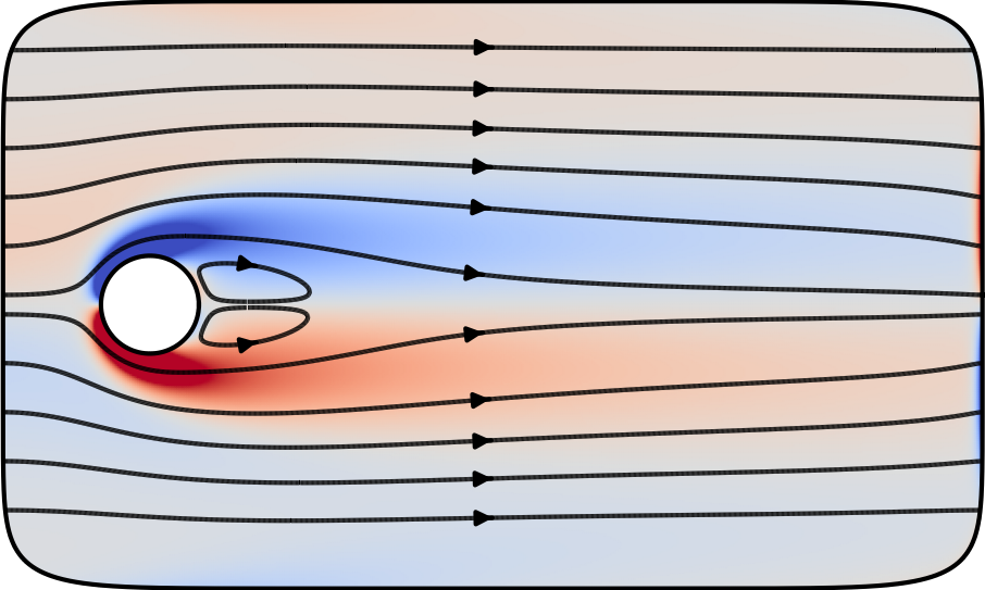
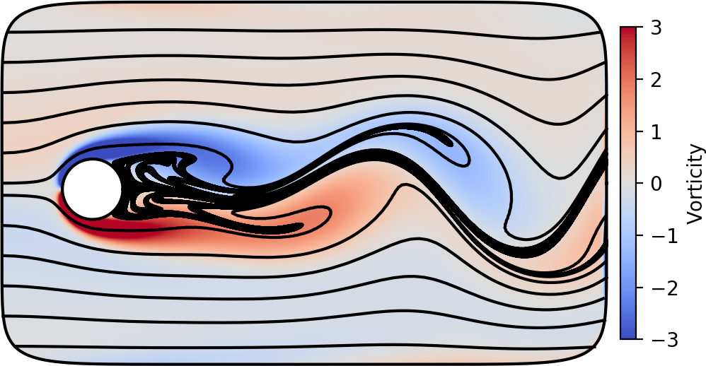
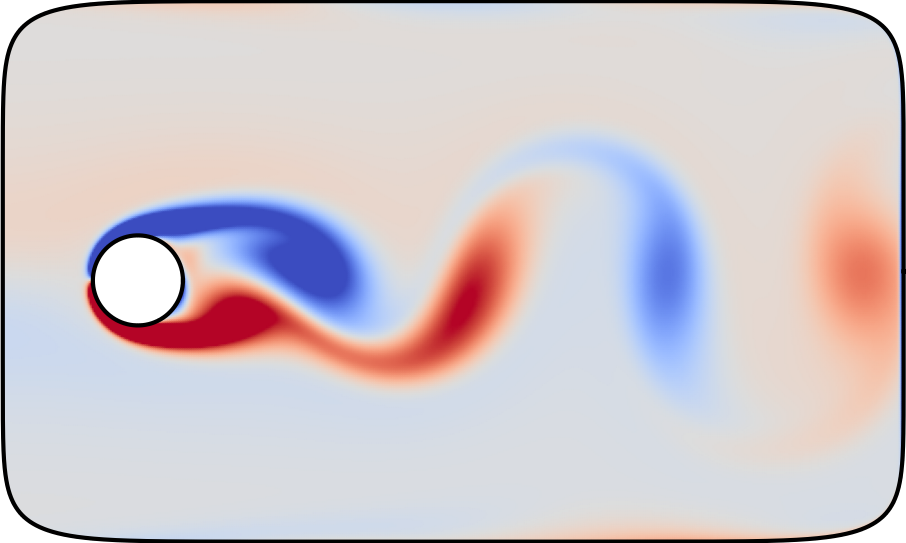
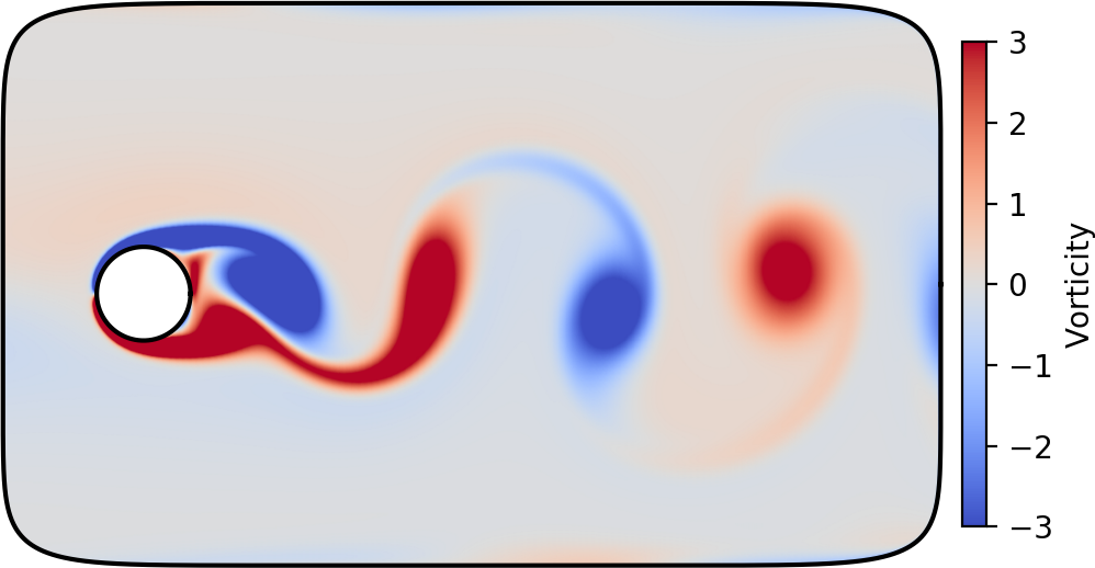
To demonstrate the effect of the Reynolds number, we consider the case of flow past a cylinder for , shown in figs. 11 and 12. We let the outer domain be the same box-shaped domain as in section 5.6, with the same slip boundary condition, and add an inclusion in the form of a circle with diameter 1 and a no-slip boundary condition. The circle is centered at ; the vertical offset is added because is reduces the number of time steps required before the vortex separation occurs.
We discretize the problem using 500 panels on the outer boundary, and 100 panels on the circle. The domain is discretized using points and PUX radius for all values of except , which is discretized using points and PUX radius , in order to get high accuracy for the larger . We time step using second order SISDC, and observe that we need to set for the solution to be stable. This is consistent with the results in section 5.5, and as a result . Each solution is timestepped until it is either steady, or the dynamics of the unsteady solution are fully developed.
The flow behind a cylinder in a free stream develops an oscillating tail of trailing vortices (a vortex street) for Reynolds numbers above the critical value, which is around 40. This is consistent with our simulation, which is steady for , and develops a vortex street for and higher. Even though it is confined to a relatively small domain, with free-stream boundary conditions at the outer boundary, the results in figs. 11 and 12 match qualitatively with other results in the literature, e.g. [57].
6 Conclusion
In the preceding we have demonstrated a fast integral equation method (FIEM) for the Navier–Stokes equations in general smooth geometries in two dimensions. The solver has a number of favorable features. In terms of accuracy, the solver is 10th-order accurate in the spatial grid spacing, and we have demonstrated up to 4th-order convergence in time. By using an embedded boundary approach combined with a uniform grid, the method can effortlessly deal with complex geometries. In addition, the use of potential methods means that the solution satisfies the incompressibility contraint by construction. This eliminates the need for projection methods, and the artificial boundary conditions associated with them. It also makes it straightforward to use off-the-shelf methods to augment the temporal accuracy of the underlying IMEX discretization, and one could easily replace the SISDC scheme with, for example, a linear multistep method based on a backward differentiation formula (BDF) discretization.
Our numerical results indicate that our method can be used to solve the unsteady Navier-Stokes equations to high accuracy, for Reynolds numbers up to at least . They do however also point towards a fundamental limitation in using a discretization based on Rothe’s method. For large values of (corresponding to large Reynolds numbers or short time steps), we see that more and more spatial resolution is needed to resolve the underlying kernels; see for instance, fig. 6. This is due to the modified Stokes equation being fundamentally harder to solve for large . Combined with the stability restriction (136), which implies the parameter scaling , this leads us to believe that our method will mainly be found useful for flows with low or moderate Reynolds numbers, in the range of hundreds up to a thousand.
For computations in two dimensions, there are several straightforward directions in which the present method can be developed. The integral equation formulation can be extended to allow for a wider class of boundary conditions, and to allow post-solution computation of various quantities, such as the pressure. While our method applies only to smooth domains, there has been recent progress in the efficient discretization of boundary integral equations on domains with corners, see, for instance, [55, 53, 37, 35]. Implementing one of these schemes would allow accurate computation of flows around geometries with sharp corners. It would also be of interest to extend our method to deal with moving geometries, such as drops, bubbles, vesicles, and particles. Here, the primary challenge would be to achieve high order accuracy while using function extension for computing the volume potential.
Although there are several ways in which the present work may be improved, we believe that the most interesting direction of development is to extend it to three dimensions (3D). Many of the tools used in this work extend directly to 3D, but not all. In particular, the panel-based, kernel-split quadrature is limited to 2D, but could be replaced by the quadrature-by-expansion (QBX) method [41, 58]. In addition, high performance computing aspects become much more important in 3D, due to the large amount of degrees of freedom, and issues of adaptivity and parallelization must be considered from the start.
Acknowledgments
The authors gratefully acknowledge support from the Knut and Alice Wallenberg Foundation under grant no. 2016.0410 (LaK), from the Air Force Office of Scientific Research under grant FA9550-17-1-0329 (TA), and from the Natural Science and Engineering Research Council of Canada (MCK). We also wish to thank Adrianna Gillman for providing us with an implementation of a fast direct solver, and Fredrik Fryklund for providing us with an implementation of PUX.
Appendix A Modified Stokes layer potentials
In this section, we provide some technical results which describe the properties of the modified Stokes double layer potential and which explain the use of the nullspace correction. We closely follow the presentation of [14]. Details and proofs may be found in [40] for the Stokes case and [52, 14] for the modified Stokes case.
For reference, the homogeneous modified Stokes equation with the Dirichlet boundary condition is given by
| (142) | ||||||
| (143) | ||||||
| (144) |
As in the main text, the divergence-free condition implies that the boundary data should satisfy
| (145) |
The following energy-type result is convenient for establishing the uniqueness of various boundary value problems for the modified Stokes equation.
Lemma 1 (Energy [14]).
The quantity is sometimes referred to as the surface traction. For the modified Stokes equation, specifying the surface traction is the natural Neumann boundary value problem. We have
Corollary 1 (Uniqueness [14]).
Corollary 2 (Uniqueness, exterior [14]).
While it was not necessary to the discussion in the main text, the modified Stokes single layer potential is useful in the discussion of jump conditions and invertibility. For a given single layer density defined on , the potential is denoted by and is defined by the boundary integral
| (147) |
where is the Stokeslet as defined in (11). Denote the stress tensor associated with the single layer potential by . Another layer potential of interest corresponds to the surface traction of the single layer potential. We denote this layer potential by , and for , it is defined by
| (148) |
where the symbol indicates that this integral is interpreted in the Cauchy principal value sense. Note that this integral operator is the transpose of the double layer operator.
The modified Stokes single and double layer potentials satisfy jump conditions which are analogous to the more familiar jump conditions for harmonic layer potentials.
Lemma 2 (Jump conditions).
Let , , , and be the layer potentials as defined above and let be a sufficiently smooth domain boundary with inward pointing normal . Then, for a given density defined on , we have that is continuous across , the exterior and interior limits of the surface traction of are equal, and for each ,
| (149) | ||||
| (150) |
Note that the integral in the definition of is interpreted in the Cauchy principal value sense when .
The above expressions are derived by noting that the leading order singularity of these integral kernels is the same as for the original Stokes case, so that the standard jump conditions for Stokes [40, 52] apply. The correspondence between the and operators, namely that , helps to characterize the nullspace of .
Lemma 3 (Nullspace [14]).
Suppose that is the boundary of a (possibly multiply-connected) bounded domain and that denotes the inward pointing normal. Then . If and , then .
In order to deal with the rank 1 nullspace described above, we add the term
| (151) |
to the double layer potential. This process is sometimes referred to as a nullspace correction or Wielandt’s deflation [14, 21]. We summarize this process in
Lemma 4 (Invertibility).
Let and be defined as above. Then, the equation
| (152) |
is uniquely invertible. Moreover, is zero provided that the right hand side satisfies the condition
| (153) |
Appendix B Free-space Green’s functions of the modified Stokes equations
We here derive the fundamental solutions to the modified Stokes equations needed for our application. Our starting point is the fundamental solution to the modified biharmonic equation,
| (156) |
In two dimensions [39],
| (157) |
where and is a modified Bessel functions of the second kind. We now seek the fundamental solution to the modified Stokes equation, such that
| (158) | ||||
| (159) |
where is an arbitrary constant. Substituting using (156) and taking the divergence,
| (160) |
such that
| (161) |
Substituting (156) and (161) into (158),
| (162) | ||||
| (163) | ||||
| (164) |
such that the stokeslet tensor is given by
| (165) |
We now switch to index notation, following the Einstein summation convention and using the notation . The Kronecker delta is not to be confused with the Dirac delta function used above. The stokeslet is then written
| (166) |
and the corresponding pressure vector is given by
| (167) |
The stresslet tensor, defined as
| (168) |
is then given by
| (169) |
Note that for we recover the corresponding tensors for regular Stokes flow, with being the fundamental solution to the biharmonic equation.
We have that is a radial function in , . Using that in dimension
| (170) |
and
| (171) |
it is straightforward to derive that
| (172) | ||||
| (173) | ||||
| (174) | ||||
| (175) | ||||
Using these relations, we can now write down , and in terms of , and ,
| (176) | ||||
| (177) | ||||
| (178) | ||||
In two dimensions (using and (157)) we can write
| (179) | ||||
| (180) | ||||
| (181) |
where
| (182) | ||||
| (183) | ||||
| (184) | ||||
| (185) | ||||
| (186) |
To avoid cancellation errors, the above expressions must be evaluated using power series for small values of the argument , see appendix C.
Appendix C Power series
In the closed-form expressions for the stokeslet and the stresslet, eqs. 179 and 181, the expressions for the functions and , eqs. 182, 183, 184, 185 and 186, are prone to cancellation errors for small arguments. To get around this, we form their power series, by combining the coefficients of the series expansions of the modified Bessel functions. The fundamental expansions needed are [48, §10.25 and §10.31]
| (187) | ||||
| (188) | ||||
| (189) | ||||
| (190) |
where is the digamma function, which be can evaluated recursively starting from the Euler-Mascheroni constant ,
| (192) | ||||
| (193) |
We write the above power series on the following compact form:
| (194) | ||||||
| (195) |
where
| (196) | ||||
| (197) | ||||
| (198) | ||||
| (199) |
In our application we only have use for the functions . These can now be computed for small using
| (200) | ||||
| (201) | ||||
| (202) |
In our code, we have empirically determined that we need to switch to power series evaluation for when , and that it is sufficient to truncate the sums to 11 terms. For the derivatives , we evaluate the derivatives of the above series when , with the sums truncated to 13 terms.
For the kernel-split quadrature described in section 4, we also need power series expansions of the smooth functions and , as defined in section 4.1. These are straightforward to break out from the above expansions, by splitting the factor from the coefficients,
| (203) |
References
- Acheson [1990] D. J. Acheson. Elementary Fluid Dynamics. Oxford University Press, New York, 1990. ISBN 9780198596790.
- af Klinteberg and Askham [2019] L. af Klinteberg and T. Askham. INSE FIEM 2D, 2019. URL https://github.com/ludvigak/inse-fiem-2d.
- af Klinteberg and Tornberg [2017] L. af Klinteberg and A.-K. Tornberg. Error estimation for quadrature by expansion in layer potential evaluation. Adv. Comput. Math., 43(1):195–234, 2017. doi: 10.1007/s10444-016-9484-x.
- af Klinteberg and Tornberg [2018] L. af Klinteberg and A.-K. Tornberg. Adaptive Quadrature by Expansion for Layer Potential Evaluation in Two Dimensions. SIAM J. Sci. Comput., 40(3):A1225–A1249, 2018. doi: 10.1137/17M1121615.
- af Klinteberg et al. [2019] L. af Klinteberg, F. Fryklund, and A.-K. Tornberg. An adaptive kernel-split quadrature method for parameter-dependent layer potentials. arXiv:1906.07713 [math.NA], 2019.
- Ascher et al. [1995] U. M. Ascher, S. J. Ruuth, and B. T. R. Wetton. Implicit-Explicit Methods for Time-Dependent Partial Differential Equations. SIAM J. Numer. Anal., 32(3):797–823, 1995. doi: 10.1137/0732037.
- Askham [2016] T. Askham. Integral-equation methods for inhomogeneous elliptic partial differential equations in complex geometry. PhD thesis, New York University, 2016.
- Askham [2018] T. Askham. A Stabilized Separation of Variables Method for the Modified Biharmonic Equation. J. Sci. Comput., 76(3):1674–1697, 2018. doi: 10.1007/s10915-018-0679-9.
- Askham and Cerfon [2017] T. Askham and A. Cerfon. An adaptive fast multipole accelerated Poisson solver for complex geometries. J. Comput. Phys., 344:1–22, 2017. doi: 10.1016/j.jcp.2017.04.063.
- Barnett [2014] A. H. Barnett. Evaluation of Layer Potentials Close to the Boundary for Laplace and Helmholtz Problems on Analytic Planar Domains. SIAM J. Sci. Comput., 36(2):A427–A451, 2014. doi: 10.1137/120900253.
- Barnett et al. [2018] A. H. Barnett, J. F. Magland, and L. af Klinteberg. A parallel non-uniform fast Fourier transform library based on an "exponential of semicircle" kernel. arXiv:1808.06736 [math.NA], 2018.
- Berrut and Trefethen [2004] J.-P. Berrut and L. N. Trefethen. Barycentric Lagrange Interpolation. SIAM Rev., 46(3):501–517, 2004. doi: 10.1137/S0036144502417715.
- Bezanson et al. [2017] J. Bezanson, A. Edelman, S. Karpinski, and V. B. Shah. Julia: A Fresh Approach to Numerical Computing. SIAM Rev., 59(1):65–98, 2017. doi: 10.1137/141000671.
- Biros et al. [2002] G. Biros, L. Ying, and D. Zorin. The embedded boundary integral method for the unsteady incompressible Navier–Stokes equations. Technical Report TR2003-838, Courant Institute, New York University, 2002.
- Björck and Pereyra [1970] A. Björck and V. Pereyra. Solution of Vandermonde Systems of Equations. Math. Comput., 24(112):893, 1970. doi: 10.2307/2004623.
- Brinkman [1947] H. C. Brinkman. A calculation of the viscous force exerted by a flowing fluid on a dense swarm of particles. Appl. Sci. Res., A1:27, 1947. doi: 10.1007/BF02120313.
- Cheng et al. [2005] H. Cheng, Z. Gimbutas, P. G. Martinsson, and V. Rokhlin. On the Compression of Low Rank Matrices. SIAM J. Sci. Comput., 26(4):1389–1404, 2005. doi: 10.1137/030602678.
- Cheng et al. [2006] H. Cheng, J. Huang, and T. J. Leiterman. An adaptive fast solver for the modified Helmholtz equation in two dimensions. J. Comput. Phys., 211(2):616–637, 2006. doi: 10.1016/j.jcp.2005.06.006.
- Dutt et al. [2000] A. Dutt, L. Greengard, and V. Rokhlin. Spectral Deferred Correction Methods for Ordinary Differential Equations. Bit Numer. Math., 40(2):241–266, 2000. doi: 10.1023/A:1022338906936.
- Fornberg et al. [2011] B. Fornberg, E. Larsson, and N. Flyer. Stable Computations with Gaussian Radial Basis Functions. SIAM J. Sci. Comput., 33(2):869–892, 2011. doi: 10.1137/09076756X.
- Frank [1958] W. L. Frank. Computing Eigenvalues of Complex Matrices by Determinant Evaluation and by Methods of Danilewski and Wielandt. J. Soc. Ind. Appl. Math., 6(4):378–392, 1958. doi: 10.1137/0106026.
- Fryklund and Lehto [2018] F. Fryklund and E. Lehto. PUXdemo, 2018. URL https://github.com/fryklund/PUXdemo.
- Fryklund et al. [2018] F. Fryklund, E. Lehto, and A.-K. Tornberg. Partition of unity extension of functions on complex domains. J. Comput. Phys., 375:57–79, 2018. doi: 10.1016/j.jcp.2018.08.012.
- Fryklund et al. [2019] F. Fryklund, M. C. A. Kropinski, and A.-K. Tornberg. An integral equation based numerical method for the forced heat equation on complex domains. arXiv:1907.08537 [math.NA], 2019.
- Gillman et al. [2012] A. Gillman, P. M. Young, and P.-G. Martinsson. A direct solver with O(N) complexity for integral equations on one-dimensional domains. Front. Math. China, 7(2):217–247, 2012. doi: 10.1007/s11464-012-0188-3.
- Gimbutas and Greengard [2017] Z. Gimbutas and L. Greengard. FMMLIB2D, 2017. URL https://github.com/zgimbutas/fmmlib2d.
- Greengard and Jiang [2018] L. Greengard and S. Jiang. A new mixed potential representation for the equations of unsteady, incompressible flow. arXiv:1809.08442 [math.NA], 2018.
- Greengard and Kropinski [1998] L. Greengard and M. C. Kropinski. An Integral Equation Approach to the Incompressible Navier–Stokes Equations in Two Dimensions. SIAM J. Sci. Comput., 20(1):318–336, 1998. doi: 10.1137/S1064827597317648.
- Greengard and Rokhlin [1987] L. Greengard and V. Rokhlin. A fast algorithm for particle simulations. J. Comput. Phys., 73(2):325–348, 1987. doi: 10.1016/0021-9991(87)90140-9.
- Greengard and Rokhlin [1997] L. Greengard and V. Rokhlin. A new version of the Fast Multipole Method for the Laplace equation in three dimensions. Acta Numer., 6:229, 1997. doi: 10.1017/S0962492900002725.
- Greengard et al. [2018] L. Greengard, S. Jiang, and J. Wang. On the accurate evaluation of unsteady Stokes layer potentials in moving two-dimensional geometries. 10010:1–17, 2018.
- Hao et al. [2014] S. Hao, A. H. Barnett, P. G. Martinsson, and P. Young. High-order accurate methods for Nyström discretization of integral equations on smooth curves in the plane. Adv. Comput. Math., 40(1):245–272, 2014. doi: 10.1007/s10444-013-9306-3.
- Helsing [2009] J. Helsing. Integral equation methods for elliptic problems with boundary conditions of mixed type. J. Comput. Phys., 228(23):8892–8907, 2009. doi: 10.1016/j.jcp.2009.09.004.
- Helsing and Holst [2015] J. Helsing and A. Holst. Variants of an explicit kernel-split panel-based Nyström discretization scheme for Helmholtz boundary value problems. Adv. Comput. Math., 41(3):691–708, 2015. doi: 10.1007/s10444-014-9383-y.
- Helsing and Jiang [2018] J. Helsing and S. Jiang. On Integral Equation Methods for the First Dirichlet Problem of the Biharmonic and Modified Biharmonic Equations in NonSmooth Domains. SIAM J. Sci. Comput., 40(4):A2609–A2630, 2018. doi: 10.1137/17M1162238.
- Helsing and Ojala [2008a] J. Helsing and R. Ojala. On the evaluation of layer potentials close to their sources. J. Comput. Phys., 227(5):2899–2921, 2008a. doi: 10.1016/j.jcp.2007.11.024.
- Helsing and Ojala [2008b] J. Helsing and R. Ojala. Corner singularities for elliptic problems: Integral equations, graded meshes, quadrature, and compressed inverse preconditioning. J. Comput. Phys., 227(20):8820–8840, 2008b. doi: 10.1016/j.jcp.2008.06.022.
- Ho et al. [2018] K. Ho, S. Olver, T. Kelman, and R. M. Slevinsky. LowRankApprox.jl, 2018. URL https://zenodo.org/record/1481098.
- Jiang et al. [2013] S. Jiang, M. C. A. Kropinski, and B. D. Quaife. Second kind integral equation formulation for the modified biharmonic equation and its applications. J. Comput. Phys., 249:113–126, 2013. doi: 10.1016/j.jcp.2013.04.034.
- Kim and Karrila [1991] S. Kim and S. J. Karrila. Microhydrodynamics : principles and selected applications. Butterworth-Heinemann series in chemical engineering. Butterworth-Heinemann, Boston, 1991. ISBN 0750691735.
- Klöckner et al. [2013] A. Klöckner, A. Barnett, L. Greengard, and M. O’Neil. Quadrature by expansion: A new method for the evaluation of layer potentials. J. Comput. Phys., 2013. doi: 10.1016/j.jcp.2013.06.027.
- Kropinski and Quaife [2011] M. C. A. Kropinski and B. D. Quaife. Fast integral equation methods for Rothe’s method applied to the isotropic heat equation. Comput. Math. with Appl., 61(9):2436–2446, 2011. doi: 10.1016/j.camwa.2011.02.024.
- Larsson [2015] E. Larsson. RBF-QR, 2015. URL http://www.it.uu.se/research/scientific_computing/software/rbf_qr.
- Liberty et al. [2007] E. Liberty, F. Woolfe, P.-G. Martinsson, V. Rokhlin, and M. Tygert. Randomized algorithms for the low-rank approximation of matrices. Proc. Natl. Acad. Sci., 104(51):20167–20172, 2007. doi: 10.1073/pnas.0709640104.
- Marple et al. [2016] G. R. Marple, A. Barnett, A. Gillman, and S. Veerapaneni. A Fast Algorithm for Simulating Multiphase Flows Through Periodic Geometries of Arbitrary Shape. SIAM J. Sci. Comput., 38(5):B740–B772, 2016. doi: 10.1137/15M1043066.
- Martinsson and Rokhlin [2005] P. Martinsson and V. Rokhlin. A fast direct solver for boundary integral equations in two dimensions. J. Comput. Phys., 205(1):1–23, 2005. doi: 10.1016/j.jcp.2004.10.033.
- Minion [2003] M. L. Minion. Semi-implicit spectral deferred correction methods for ordinary differential equations. Commun. Math. Sci., 1(3):471–500, 2003. doi: 10.4310/CMS.2003.v1.n3.a6.
- NIST [2017] NIST. Digital Library of Mathematical Functions. Release 1.0.16, 2017. URL http://dlmf.nist.gov/.
- Ojala and Tornberg [2015] R. Ojala and A.-K. Tornberg. An accurate integral equation method for simulating multi-phase Stokes flow. J. Comput. Phys., 298:145–160, 2015. doi: 10.1016/j.jcp.2015.06.002.
- Peskin [2002] C. S. Peskin. The immersed boundary method. Acta Numer., 11(2002):479–517, 2002. doi: 10.1017/S0962492902000077.
- Pozrikidis [1989] C. Pozrikidis. A singularity method for unsteady linearized flow. Phys. Fluids A Fluid Dyn., 1(9):1508–1520, 1989. doi: 10.1063/1.857329.
- Pozrikidis [1992] C. Pozrikidis. Boundary Integral and Singularity Methods for Linearized Viscous Flow. Cambridge University Press, Cambridge, 1992. ISBN 9780511624124. doi: 10.1017/CBO9780511624124. URL http://ebooks.cambridge.org/ref/id/CBO9780511624124.
- Rachh and Serkh [2017] M. Rachh and K. Serkh. On the solution of Stokes equation on regions with corners. arXiv:1711.04072 [math-ph], 2017.
- Saad and Schultz [1986] Y. Saad and M. H. Schultz. GMRES: A Generalized Minimal Residual Algorithm for Solving Nonsymmetric Linear Systems. SIAM J. Sci. Stat. Comput., 7(3):856–869, 1986. doi: 10.1137/0907058.
- Serkh and Rokhlin [2016] K. Serkh and V. Rokhlin. On the solution of elliptic partial differential equations on regions with corners. J. Comput. Phys., 305:150–171, 2016. doi: 10.1016/j.jcp.2015.10.024.
- Stein et al. [2017] D. B. Stein, R. D. Guy, and B. Thomases. Immersed Boundary Smooth Extension (IBSE): A high-order method for solving incompressible flows in arbitrary smooth domains. J. Comput. Phys., 335:155–178, 2017. doi: 10.1016/j.jcp.2017.01.010.
- Tafuni et al. [2018] A. Tafuni, J. Domínguez, R. Vacondio, and A. Crespo. A versatile algorithm for the treatment of open boundary conditions in Smoothed particle hydrodynamics GPU models. Comput. Methods Appl. Mech. Eng., 342:604–624, 2018. doi: 10.1016/j.cma.2018.08.004.
- Wala and Klöckner [2019] M. Wala and A. Klöckner. A fast algorithm for Quadrature by Expansion in three dimensions. J. Comput. Phys., 388:655–689, 2019. doi: 10.1016/j.jcp.2019.03.024.
- Wang and Greengard [2019] J. Wang and L. Greengard. Hybrid asymptotic/numerical methods for the evaluation of layer heat potentials in two dimensions. Adv. Comput. Math., 45(2):847–867, 2019. doi: 10.1007/s10444-018-9641-5.