Secrecy Preserving in Stochastic Resource Orchestration for Multi-Tenancy Network Slicing

To keep up with the proliferation of wireless services, new cell sites are being constantly built, eventually leading to dense network deployments [1]. However, it becomes extremely complex to operate the control plane functions in a dense radio access network (RAN). In recent years, the computation-intensive applications (e.g., augmented reality and interactive online gaming) are gaining increasing popularity [2]. The mobile user (MU)-end terminal devices are in general constrained by battery capacity and processing speed of the central processing unit (CPU). The tension between computation-intensive applications and resource-constrained terminal devices calls for a revolution in computing [3]. Mobile-edge computing (MEC) is envisioned as a promising solution, which brings the computing capabilities within the RANs in close proximity to MUs [2]. Offloading a computation task to a MEC server for execution involves data transmissions. How to orchestrate radio resources between MEC and traditional mobile services adds another dimension of complexity to the network operations [4]. By abstracting all physical base stations (BSs) in a geographical area as a logical big BS, the software-defined networking (SDN) concept provides infrastructure flexibility as well as service-oriented customization [5]. In a software-defined RAN, the SDN-orchestrator handles all control plane operations.

One key benefit from a software-defined RAN is to facilitate network sharing [6]. As such, the same physical network is able to host multiple service providers (SPs, namely, multiple tenants [7]), which breaks the traditional business model regarding the single ownership of a network infrastructure [8]. For example, an over-the-top application provider (e.g., Google [9]) can be a SP so as to lease radio resources from the infrastructure provider to improve the Quality-of-Service and the Quality-of-Experience for its subscribers. Building upon the 3GPP TSG SA 5 network sharing paradigm [10], a software-defined RAN architecture and its integration with network function virtualization enable RAN-only slicing that splits the RAN into multiple virtual slices [11]. This paper is primarily concerned with a software-defined RAN where the RAN slices are specifically tailored to accommodate both computation and communication functionalities [12].

The technical challenges yet remain for the implementation of RAN-only slicing. Particularly, the mechanisms that exploit the decoupling of control and data planes in a software-defined RAN must be developed to optimize radio resource utilization. For the considered software-defined RAN, a limited number of channels are auctioned over the time horizon to the MUs, which request MEC and traditional mobile services. An eavesdropper exists in the network and overhears the MUs during the data transmissions [13]. Multiple SPs compete to orchestrate the channels for their subscribed MUs according to the network dynamics, aiming to maximize the expected long-term payoff performance. Upon receiving the auction bids from all SPs, the SDN-orchestrator allocates channels to the MUs through a Vickrey-Clarke-Groves (VCG) mechanism¹¹ 1 The VCG mechanism ensures truthfulness, efficiency and incentive compatibility. [14]. To combat the threat from the eavesdropper, each MU then proceeds to use a secrecy-rate [13] to offload computation tasks and schedule packets over the assigned channel. To the best of our knowledge, there does not exist a comprehensive study on stochastic resource orchestration in multi-tenancy RAN-only slicing with secrecy preserving.

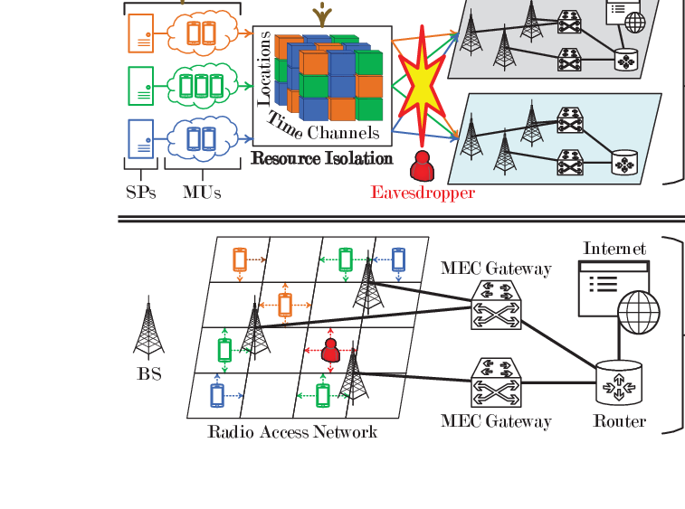
As shown in Fig. 1, we focus on a system model with RAN-only slicing, where an eavesdropper intentionally overhears the data transmissions of the MUs. The time horizon is divided into discrete scheduling slots, each of which is indexed by an integer $k\in\mathds{N}_{+}$ and is assumed to be of equal duration $\delta$ (in seconds). The RAN consists of a set $\mathcal{B}$ of physical BSs covering a service area, which can be represented by a set $\mathcal{L}$ of small locations with each being characterized by uniform signal propagation conditions [15]. We use $\mathcal{L}_{b}$ to denote the serving area of a BS $b\in B$. For any two BSs $b$ and $b^{\prime}\in\mathcal{B}$ ($b^{\prime}\neq b$), we assume that $\mathcal{L}_{b}\cap\mathcal{L}_{b^{\prime}}=\emptyset$. We denote the geographical distribution of BSs by a topological graph $\mathcal{TG}=\langle\mathcal{B},\mathcal{E}\rangle$, where $\mathcal{E}=\{e_{b,b^{\prime}}:b\neq b^{\prime},b,b^{\prime}\in\mathcal{B}\}$ with $e_{b,b^{\prime}}=1$ if BSs $b$ and $b^{\prime}$ are neighbours and otherwise $e_{b,b^{\prime}}=0$. Suppose that $I$ SPs provide both MEC and traditional mobile services to MUs while each MU can subscribe to only one SP. Let $\mathcal{N}_{i}$ be the set of MUs of a SP $i\in\mathcal{I}=\{1,\cdots,I\}$.

Across the scheduling slots, the MUs and the eavesdropper move within $\mathcal{L}$ following a Markov mobility model [16]. Denote by $\mathcal{N}_{b,i}^{k}$ the set of MUs of SP $i\in\mathcal{I}$ moving into the area of a BS $b\in\mathcal{B}$ during a slot $k$. We assume that a MU at a location can only be associated with the BS that covers the location. In the network, all MUs share a set $\mathcal{J}=\{1,\cdots,J\}$ of orthogonal channels with the same bandwidth $\eta$ (in Hz). The SPs compete for the limited channel access opportunities for their MUs. Specifically, at the beginning of a scheduling slot $k$, each SP $i$ submits an auction bid $\bm{\beta}_{i}^{k}=(\nu_{i}^{k},\mathbf{C}_{i}^{k})$, where $\nu_{i}^{k}$ is the valuation over $\mathbf{C}_{i}^{k}=(C_{b,i}^{k}:b\in\mathcal{B})$ with $C_{b,i}^{k}$ being the number of requested channels in the service area of a BS $b$. After receiving $\bm{\beta}^{k}=(\bm{\beta}_{i}^{k}:i\in\mathcal{I})$, the SDN-orchestrator performs channel allocation and calculates payment $\tau_{i}^{k}$ for each SP $i$. Let $\bm{\rho}_{n}^{k}=(\rho_{n,j}^{k}:j\in\mathcal{J})$ be the channel allocation of a MU $n\in\mathcal{N}=\cup_{i\in\mathcal{I}}\mathcal{N}_{i}$, where $\rho_{n,j}^{k}=1$ if channel $j$ is allocated to MU $n\in\mathcal{N}$ during slot $k$ and $\rho_{n,j}^{k}=0$, otherwise. We also apply the following constraints for centralized channel allocation at the SDN-orchestrator during a slot,

which ensure that one channel cannot be allocated to MUs associated with two adjacent BSs in order to avoid interference during data transmissions, while in the service area of a BS, one MU can be assigned at most one channel and one channel can be assigned to at most one MU. Denote $\bm{\phi}^{k}=(\phi_{i}^{k}:i\in\mathcal{I})$ as the winner vector at the beginning of a scheduling slot $k$, where $\phi_{i}^{k}=1$ if SP $i$ wins the channel auction and $\phi_{i}^{k}=0$ indicates that no channel will be allocated to the MUs of SP $i$ during the slot. The SDN-orchestrator determines $\bm{\phi}^{k}$ via the VCG pricing mechanism, namely,

where $\varphi_{n}^{k}=\sum_{j\in\mathcal{J}}\rho_{n,j}^{k}$ and $\bm{\phi}=(\phi_{i}:i\in\mathcal{I})$ with $\phi_{i}\in\{0,1\}$. The payment $\tau_{i}^{k}$ for each SP $i$ can be calculated to be $\tau_{i}^{k}=\max_{\bm{\phi}_{-i}}\sum_{i^{\prime}\in\mathcal{I}\setminus\{i\}}\phi_{i^{\prime}}\cdot\nu_{i^{\prime}}^{k}-\max_{\bm{\phi}}\sum_{i^{\prime}\in\mathcal{I}\setminus\{i\}}\phi_{i^{\prime}}\cdot\nu_{i^{\prime}}^{k}$, where $-i$ denotes all the competitors of SP $i$.

Let $L_{n,(\mathrm{u})}^{k}$ and $L_{(\mathrm{e})}^{k}\in\mathcal{L}$ be the geographical locations of a MU $n\in\mathcal{N}$ and the eavesdropper during a scheduling slot $k$, respectively. As in [15], we assume that the average channel gains $H_{n,(\mathrm{u})}^{k}=h_{(\mathrm{u})}(L_{n,(\mathrm{u})}^{k})$ and $H_{n,(\mathrm{e})}^{k}=h_{(\mathrm{e})}(L_{n,(\mathrm{u})}^{k},L_{(\mathrm{e})}^{k})$ of links between MU $n$ and the associated BS as well as the eavesdropper are determined by the respective distances. At the beginning of each scheduling slot $k$, MU $n$ independently generates a random number $A_{n,(\mathrm{t})}^{k}\in\mathcal{A}=\{0,1,\cdots,A_{(\mathrm{t})}^{(\max)}\}$ of computation tasks²² 2 To ease analysis, we assume that the maximum CPU power at a mobile device matches the maximum computation task arrivals and a MU can process $A_{(\mathrm{t})}^{(\max)}$ tasks within one scheduling slot. according to a Markov process [17]. We represent a computation task by $(\mu_{(\mathrm{t})},\vartheta)$, where $\mu_{(\mathrm{t})}$ and $\vartheta$ are, respectively, the input data size (in bits) and the number of CPU cycles required to accomplish one input bit of the computation task. For a computation task, two decisions are available: 1) to be processed locally at the MU; or 2) to be offloaded to the MEC server in the computation slice for execution. The computation offloading decision for MU $n$ at a slot $k$ specifies the number $R_{n,(\mathrm{t})}^{k}$ of tasks to be transmitted to the MEC server. Then the remaining $A_{n,(\mathrm{t})}^{k}-\varphi_{n}^{k}\cdot R_{n,(\mathrm{t})}^{k}$ tasks are to be processed locally. Meanwhile, a data queue at a MU buffers the packets from the traditional mobile service. Let $W_{n}^{k}$ and $A_{n,(\mathrm{p})}^{k}$ be the queue length and the random new packet arrivals for MU $n$ at the beginning of a slot $k$. We assume that the data packets are of a constant size $\mu_{(\mathrm{p})}$ (bits) and the packet arrival process is independent among the MUs and identical and independently distributed across time. Let $R_{n,(\mathrm{p})}^{k}$ be the number of packets that are scheduled for transmission from MU $n$ at scheduling slot $k$. The queue evolution of MU $n$ can be written as the form below,

where $W^{(\max)}$ is the queue length limit.

To ensure security, the energy (in Joules) consumed by a MU $n\in\mathcal{N}$ for transmitting $\varphi_{n}^{k}\cdot R_{n,(\mathrm{t})}^{k}$ computation tasks and $\varphi_{n}^{k}\cdot R_{n,(\mathrm{p})}^{k}$ data packets with a secrecy-rate [13] during a slot $k$ can be calculated as

where $\sigma^{2}$ is the background noise power spectral density. Let $\Omega^{(\max)}$ be the maximum transmit power for all MUs, namely, $P_{n,(\mathrm{tr})}^{k}\leq\Omega^{(\max)}\cdot\delta$, $\forall n$ and $\forall k$. For the remaining $A_{n,(\mathrm{t})}^{k}-\varphi_{n}^{k}\cdot R_{n,(\mathrm{t})}^{k}$ computation tasks that are to be locally processed, the CPU energy consumption is

where $\varsigma$ is the effective switched capacitance [18] and $\varrho$ is the CPU-cycle frequency of the MU-end devices.

At a scheduling slot $k$, the local state of a MU $n\in\mathcal{N}$ is described as $\bm{\chi}_{n}^{k}=(L_{n,(\mathrm{u})}^{k},L_{(\mathrm{e})}^{k},A_{n,(\mathrm{t})}^{k},W_{n}^{k})\in\mathcal{X}=\mathcal{L}^{2}\times$ $\mathcal{A}\times\mathcal{W}$, where the SDN-orchestrator broadcasts the information of $L_{(\mathrm{e})}^{k}$ to all MUs. Then $\bm{\chi}^{k}=(\bm{\chi}_{n}^{k}:n\in\mathcal{N})\in\mathcal{X}^{|\mathcal{N}|}$ characterizes the global network state, where $|\mathcal{N}|$ means the cardinality of the set $\mathcal{N}$. Define by $\bm{\pi}_{i}=(\pi_{i,(\mathrm{c})},\bm{\pi}_{i,(\mathrm{t})},\bm{\pi}_{i,(\mathrm{p})})$ a control policy of a SP $i\in\mathcal{I}$, where $\pi_{i,(\mathrm{c})}$, $\bm{\pi}_{i,(\mathrm{t})}=(\pi_{n,(\mathrm{t})}:n\in\mathcal{N}_{i})$ and $\bm{\pi}_{i,(\mathrm{p})}=(\pi_{n,(\mathrm{p})}:n\in\mathcal{N}_{i})$ are the channel auction, the computation offloading and the packet scheduling policies, respectively. The joint control policy of all SPs is given by $\bm{\pi}=(\bm{\pi}_{i}:i\in\mathcal{I})$. With the observation of $\bm{\chi}^{k}$ at the beginning of each scheduling slot $k$, SP $i$ announces the auction bid $\bm{\beta}_{i}^{k}$ to the SDN-orchestrator and decides the $\mathbf{R}_{i,(\mathrm{t})}^{k}$ computation tasks as well as $\mathbf{R}_{i,(\mathrm{p})}^{k}$ packets to be transmitted following $\bm{\pi}_{i}$. That is, $\bm{\pi}_{i}(\bm{\chi}^{k})=(\pi_{i,(\mathrm{c})}(\bm{\chi}^{k}),\bm{\pi}_{i,(\mathrm{t})}(\bm{\chi}_{i}^{k}),\bm{\pi}_{i,(\mathrm{p})}(\bm{\chi}_{i}^{k}))=(\bm{\beta}_{i}^{k},\mathbf{R}_{i,(\mathrm{t})}^{k},\mathbf{R}_{i,(\mathrm{p})}^{k})$, where $\mathbf{R}_{i,(\mathrm{t})}^{k}=(R_{n,(\mathrm{t})}^{k}:n\in\mathcal{N}_{i})$ and $\mathbf{R}_{i,(\mathrm{p})}^{k}=(R_{n,(\mathrm{p})}^{k}:n\in\mathcal{N}_{i})$. Accordingly, SP $i$ realizes an instantaneous payoff

where $\bm{\varphi}_{i}^{k}=(\varphi_{n}^{k}:n\in\mathcal{N}_{i})$ and $\alpha_{n}\in\mathds{R}_{+}$ is the unit price to charge a MU $n$ for achieving utility

In (III), $D_{n}^{k}=\max\{W_{n}^{k}-\varphi_{n}^{k}\cdot R_{n,(\mathrm{p})}^{k}+A_{n,(\mathrm{p})}^{k}-W^{(\max)},0\}$ defines the number of packet drops, $U_{n}^{(1)}(\cdot)$, $U_{n}^{(2)}(\cdot)$, $U_{n}^{(3)}(\cdot)$ and $U_{n}^{(4)}(\cdot)$ are the positive and monotonically decreasing functions, and $\ell_{n}\in\mathds{R}_{+}$ is a weighting factor. Obviously, the randomness lying in $\{\bm{\chi}^{k}:k\in\mathds{N}_{+}\}$ is Markovian.

Taking expectation with respect to the sequence of per-slot instantaneous payoffs, the expected long-term payoff of a SP $i\in\mathcal{I}$ for a given initial global network state $\bm{\chi}^{1}=\bm{\chi}\triangleq(\bm{\chi}_{n}=(L_{n,(\mathrm{u})},L_{(\mathrm{e})},A_{n,(\mathrm{t})},W_{n}):n\in\mathcal{N})$ can be expressed as in (12),

where $\gamma\in[0,1)$ is a discount factor. $V_{i}(\bm{\chi},\bm{\pi})$ is also termed as the state-value function of SP $i$. The aim of each SP $i$ is to device a best-response control policy $\bm{\pi}_{i}^{*}$ such that $\bm{\pi}_{i}^{*}=\arg\max_{\bm{\pi}_{i}}V_{i}(\bm{\chi},\bm{\pi}_{i},\bm{\pi}_{-i})$, $\forall\bm{\chi}\in\mathcal{X}^{|\mathcal{N}|}$. Due to the limited number of channels and the stochastic nature in networking environment, we formulate the interactions among multiple non-cooperative SPs over the scheduling slots as a stochastic game, $\mathcal{SG}$, in which $I$ SPs are the players and there are a set $\mathcal{X}^{|\mathcal{N}|}$ of global network states and a collection of control policies $\{\bm{\pi}_{i}:\forall i\in\mathcal{I}\}$. A Nash equilibrium (NE), which is a tuple of control policies $\langle\bm{\pi}_{i}^{*}:i\in\mathcal{I}\rangle$, describes the rational behaviours of the SPs in a $\mathcal{SG}$. For the $I$-player $\mathcal{SG}$ with expected infinite-horizon discounted payoffs, there always exists a NE in stationary control policies [19]. Define $\mathds{V}_{i}(\bm{\chi})=V_{i}(\bm{\chi},\bm{\pi}_{i}^{*},\bm{\pi}_{-i}^{*})$ as the optimal state-value function, $\forall i\in\mathcal{I}$ and $\forall\bm{\chi}\in\mathcal{X}^{|\mathcal{N}|}$.

From (12), it can be easily observed that the expected long-term payoff of a SP $i\in\mathcal{I}$ depends on information of not only the global network state across the scheduling slots but also the joint control policy $\bm{\pi}$. In other words, the decision makings from the non-cooperative SPs are coupled in the $\mathcal{SG}$, which makes it a challenging task to find the NE. In this section, we elaborate on how the SPs play the $\mathcal{SG}$ only with limited local information.

This section conducts numerical experiments based on TensorFlow [26] to quantify the performance of the derived DRL-based scheme for multi-tenant cross-slice resource orchestration with secrecy preserving in a software-defined RAN. We set up an experimental network with $4$ BSs being placed at equal distance $1$ Km apart in the centre of a $2\times 2$ Km² square service area [15]. The entire area is divided into $1600$ locations with each of 50$\times$50 m². The average channel gains for a MU $n\in\mathcal{N}$ at the location $L_{n,(\mathrm{u})}^{k}\in\mathcal{L}_{b}$ covered by a BS $b\in\mathcal{B}$ during a slot $k$ are given by $h_{(\mathrm{u})}(L_{n,(\mathrm{u})}^{k})=H_{0}\cdot(\xi_{0}/\xi_{b,n}^{k})^{4}$ and $h_{(\mathrm{e})}(L_{n,(\mathrm{u})}^{k},L_{(\mathrm{e})}^{k})=H_{0}\cdot(\xi_{0}/\xi_{n,(\mathrm{e})}^{k})^{4}$, where $H_{0}=-40$ dB is the path-loss constant, $\xi_{0}=2$ m is the reference distance, while $\xi_{b,n}^{k}$ and $\xi_{n,(\mathrm{e})}^{k}$ are the distances between MU $n$ and BS $b$ as well as the eavesdropper [27]. The mobilities of all MUs as well as the eavesdropper and the computation task arrivals of all MUs are independently and randomly generated. The packet arrivals follow a Poisson arrival process with average rate $\lambda$ (in packets/slot). For the utility function in (III), we select $U_{n}^{(1)}(W_{n}^{k+1})=\exp\{-W_{n}^{k+1}\}$, $U_{n}^{(2)}(D_{n}^{k})=\exp\{-D_{n}^{k}\}$, $U_{n}^{(3)}(P_{n,(\mathrm{CPU})}^{k})=\exp\{-P_{n,(\mathrm{CPU})}^{k}\}$ and $U_{n}^{(4)}(P_{n,(\mathrm{tr})}^{k})=\exp\{-P_{n,(\mathrm{tr})}^{k}\}$. We design for each MU a DQN with $2$ hidden layers with each consisting of $16$ neurons. Other parameter values used in the experiments are listed in Table I.

For comparison purpose, three baseline schemes are developed and simulated, namely,

1. 1.

   Channel-aware control policy (Baseline 1) – At the beginning of each slot $k$, the need of getting one channel at a MU $n\in\mathcal{N}$ is evaluated by $H_{n,(\mathrm{u})}^{k}-H_{(\mathrm{e})}^{k}$;

2. 2.

   Queue-aware control policy (Baseline 2) – Each MU calculates the preference between having one channel or not using a predefined threshold of the queue length;

3. 3.

   Random control policy (Baseline 3) – This policy randomly generates the value of obtaining one channel for each MU at the beginning of each slot.

With the three baselines, after the centralized channel allocation by the SDN-orchestrator at the beginning of each slot, a MU proceeds to offload a random number of computation tasks and schedule a maximum feasible number of data packets if being assigned a channel.

We first demonstrate the average utility performance per MU per scheduling slot achieved from the proposed DRL-based scheme and the three baselines under different average packet arrival rates. In this experiment, we assume that $J=11$ channels are shared among the MUs for the access to the computation and communication slices. The results are depicted in Fig. 2, from which we can observe that the proposed scheme achieves a significant performance gain. However, the average utility performance deceases as the average number of random data packet arrivals increases. The reason behind is that in order to ensure secrecy, more data packet arrivals lead to larger queue length, more packet drops and higher energy consumption across the MUs. Then in Fig. 3, we exhibit the average utility performance versus the number of channels, where the average packet arrival rate is fixed to be $\lambda=8$. More channels available in the system provide more opportunities for the MUs to transmit the data of computation tasks to be offloaded and scheduled packets. Hence better average utility performance can be expected by the MUs. When there are sufficient channels in the network, the data transmissions of all MUs with secrecy preserving can be fully satisfied. Both experiments show that the proposed scheme outperforms the three baselines.

In this paper, we investigate the problem of non-cooperative multi-tenant cross-slice resource orchestration with secrecy preserving in a software-defined RAN, which is formulated as a $\mathcal{SG}$. To alleviate private information exchange among the competing SPs, we approximate the $\mathcal{SG}$ by a $\mathcal{AG}$. Each SP is thus able to behave independently only with the local information. We observe that the decisions of the channel auction and the computation offloading as well as packet scheduling are sequentially made. This motivates us to linearly decompose the per-SP single-agent MDP, which greatly simplifies the decision making process at a SP. We propose a DRL-based scheme to find the optimal abstract control policies. Numerical experiments showcase that the performance achieved from our scheme outperforms the other baselines.

References

- [1] J. G. Andrews et al., “Femtocells: Past, present, and future,” IEEE J. Sel. Areas Commun., vol. 30, no. 3, pp. 497–508, Apr. 2012.
- [2] Y. Mao et al., “A Survey on mobile edge computing: The communication perspective,” IEEE Commun. Surveys Tuts., vol. 19, no. 4, pp. 2322–2358, Q4 2017.
- [3] M. Satyanarayanan, “The emergence of edge computing,” IEEE Comput., vol. 50, no. 1, pp. 30–39, Jan. 2017.
- [4] Y. Zhou et al., “Resource allocation for information-centric virtualized heterogeneous networks with in-network caching and mobile edge computing,” IEEE Trans. Veh. Technol., vol. 66, no. 12, pp. 11339–11351, Dec. 2017.
- [5] A. Gudipati et al., “SoftRAN: Software defined radio access network,” in ACM SIGCOMM HotSDN Workshop, Hong Kong, China, Aug. 2013.
- [6] C. Liang and F. R. Yu, “Wireless network virtualization: A survey, some research issues and challenges,” IEEE Commun. Surveys Tuts., vol. 17, no. 1, pp. 358–380, Q1 2015.
- [7] Y. Xiao and M. Krunz, “Dynamic network slicing for scalable fog computing systems with energy harvesting,” IEEE J. Sel. Areas Commun., vol. 36, no. 12, pp. 2640–2654, Dec. 2018.
- [8] T. Frisanco et al., “Infrastructure sharing and shared operations for mobile network operators: From a deployment and operations view,” in IEEE NOMS, Salvador, Bahia, Brazil, Apr. 2008.
- [9] Google, “Project Fi,” https://fi.google.com [Date Accessed: 12 Dec. 2018].
- [10] “Telecommunication management; network sharing; concepts and requirements,” Rel. 15, 3GPP TS 32.130, Jun. 2018.
- [11] O. Sallent et al., “On radio access network slicing from a radio resource management perspective,” IEEE Wireless Commun., vol. 24, no. 5, pp. 166–174, Oct. 2017.
- [12] H. Shah-Mansouri, V. W. S. Wong, and R. Schober, “Joint optimal pricing and task scheduling in mobile cloud computing systems,” IEEE Trans. Wireless Commun., vol. 16, no. 8, pp. 5218–5232, Aug. 2017.
- [13] Y. Wu et al., “Secrecy-based energy-efficient data offloading via dual connectivity over unlicensed apectrums,” IEEE J. Sel. Areas Commun., vol. 34, no. 12, pp. 3252–3270, Dec. 2016.
- [14] Z. Ji and K. J. R. Liu, “Dynamic spectrum sharing: A game theoretical overview,” IEEE Commun. Mag., vol. 45, no. 5, pp. 88–94, May 2007.
- [15] X. Chen et al., “Energy-efficiency oriented traffic offloading in wireless networks: A brief survey and a learning approach for heterogeneous cellular networks,” IEEE J. Sel. Areas Commun., vol. 33, no. 4, pp. 627–640, Apr. 2015.
- [16] A. J. Nicholson and B. D. Noble, “BreadCrumbs: Forecasting mobile connectivity,” in Proc. ACM MobiCom, San Francisco, CA, Sep. 2008.
- [17] X. He et al., “Privacy-aware offloading in mobile-edge computing,” in Proc. IEEE GLOBECOM, Singapore, Dec. 2017.
- [18] T. D. Burd and R. W. Brodersen, “Processor design for portable systems,” J. VLSI Signal Process. Syst., vol. 13, no. 2–3, pp. 203–221, Aug. 1996.
- [19] A. M. Fink, “Equilibrium in a stochastic -person game,” J. Sci. Hiroshima Univ. Ser. A-I, vol. 28, pp. 89–93, 1964.
- [20] X. Chen et al., “Wireless resource scheduling in virtualized radio access networks using stochastic learning,” IEEE Trans. Mobile Comput., vol. 17, no. 4, pp. 961–974, Apr. 2018.
- [21] J. Jia et al., “Revenue generation for truthful spectrum auction in dynamic spectrum access,” in Proc. ACM MobiHoc, New Orleans, LA, May 2009.
- [22] R. S. Sutton and A. G. Barto, Reinforcement Learning: An Introduction. Cambridge, MA: MIT Press, 1998.
- [23] V. Mnih et al., “Human-level control through deep reinforcement learning,” Nature, vol. 518, no. 7540, pp. 529–533, Feb. 2015.
- [24] H. van Hasselt, A. Guez, and D. Silver, “Deep reinforcement learning with double Q-learning,” in Proc. AAAI, Phoenix, AZ, Feb. 2016.
- [25] L.-J. Lin, “Reinforcement learning for robots using neural networks,” Carnegie Mellon University, 1992.
- [26] M. Abadi et al., “Tensorflow: A system for large-scale machine learning,” in Proc. OSDI, Savannah, GA, Nov. 2016.
- [27] Y. Mao, J. Zhang, and K. B. Letaief, “Dynamic computation offloading for mobile-edge computing with energy harvesting devices,” IEEE J. Sel. Areas Commun., vol. 34, no. 12, pp. 3590–3605, Dec. 2016.
- [28] K. Jarrett et al., “What is the best multi-stage architecture for object recognition?” in Proc. IEEE ICCV, Kyoto, Japan, Sep.–Oct. 2009.
- [29] D. P. Kingma and J. Ba, “Adam: A Method for Stochastic Optimization,” in Proc. ICLR, San Diego, CA, May 2015.