Multiple backward Schramm–Loewner evolution and coupling with Gaussian free field

Recent studies on Schramm–Loewner evolution (SLE) coupled with two-dimensional Gaussian free field (GFF) [Dub09, SS09, SS13, IK13, DMS14, She16, MS16a, MS16b, MS16c, MS17] have created a new trend in random geometry leading to a canonical construction of SLE from GFF and an insight into underlying geometry of GFF. In these studies, a GFF is an ingredient of random objects such as a quantum surface [DMS14, She16] or an imaginary surface [MS16a, MS16b, MS16c, MS17], roughly, the former (resp. the latter) of which is an equivalence class of two-dimensional simply connected domains equipped with random metrics (resp. random vector fields). Given a quantum surface uniformized to the complex upper half plane, then, one can think of matching boundary segments lying on both sides of the origin so that they have the same length with respect to the random metric and gluing them together. Consequently, one obtains a random curve growing in the complex upper half plane and could consider the conformal welding problem that requires us to determine its probability law. In the case that an imaginary surface uniformized to the complex upper half plane is given, one sees a flow line starting at the origin along the random vector field and could consider the flow line problem that requires us to determine its probability law. It has been proved [She16, MS16a, MS16b, MS16c, MS17] that, for a quantum surface and an imaginary surface with proper boundary perturbations, both problems are solved by SLE relying on the coupling of SLE with GFF.

Due to the boundary perturbations, the quantum surfaces (resp. the imaginary surfaces) subject to the conformal welding problem (resp. the flow line problem) can be regarded as being equipped with two marked boundary points (resp. boundary condition changing points) at the origin and infinity. Therefore, it seems natural to consider analogues of these problems in the case when the quantum surfaces (resp. the imaginary surfaces) are equipped with more marked boundary points (resp. boundary condition changing points) than two. In the previous work [KK20a], we posed such generalizations and found that they are solved by multiple SLE [BBK05, Dub06, Dub07, Gra07, KP16, PW19], but we also encountered a new problem.

The couplings of SLE with GFF to solve the conformal welding problem and the flow line problem are slightly different. While, in the case of the flow line problem, the coupling of the usual forward flow of SLE [Sch00, RS05] and GFF under proper boundary condition is useful, in the case of the conformal welding problem, one has to make a backward SLE coupled with a free boundary GFF with a proper boundary perturbation. These differences not only persist when we move on to the case with multiple marked boundary points/boundary condition changing points, but also get more serious. It is known [Law09b] that a forward SLE and a backward SLE are roughly the inverse mapping of each other, which is why a forward SLE and a backward SLE generate essentially the same random curve. Note that the proof of this fact relies on the property that, for a Brownian motion $(B_{t}:t\geq 0)$ and a fixed time $T>0$, the stochastic process $(B_{T-t}-B_{T}:t\in[0,T])$ is again a Brownian motion. Therefore, for a multiple SLE, whose driving process has a drift term apart from a Brownian motion, the same thing cannot be expected. Nevertheless, a multiple backward SLE naturally gives a solution to the conformal welding problem for a quantum surface with multiple marked boundary points. The new problem mentioned above and that we address in this paper is how a multiple backward SLE makes sense as a stochastic process generating random curves.

Let us take a quick look at construction of a multiple SLE in forward case based on the commutation relation between Loewner chains [Dub06, Dub07, Gra07]. Suppose that we have two Loewner chains $\left(g_{t}(\cdot):t\geq 0\right)$ and $\left(\tilde{g}_{s}(\cdot):s\geq 0\right)$ driven by some Itô processes. Using these Loewner chains, one can think of two schemes of generating multiple curves: One scheme is to generate a curve according to $\left(g_{t}(\cdot):t\geq 0\right)$ and next to generate the other curve in the remaining domain letting $\left(\tilde{g}_{s}(\cdot):s\geq 0\right)$ evolve, and the other one is to do the same thing in the converted order. In both schemes, one obtains two random curves in the complex upper half plane. Then, the requirement that their probability laws are identical imposes strict conditions on the driving processes of the Loewner chains. In particular, it can be argued that they share a function that solves a system of Belavin–Polyakov–Zamolodchikov(BPZ)-like equations so that their drift terms are given by its logarithmic derivatives. What is called a multiple SLE these days [KP16, PW19] is a multiple of Loewner chains, the driving process of each of which has a drift term given by a logarithmic derivative of a single function solving a system of BPZ equations. Owing to the argument of the commutation relation, it is ensured that these Loewner chains consistently generate multiple curves in the complex half plane. It is also known [Wer04, SW05, KP16, PW19] that, for a multiple SLE, each Loewner chain is a Girsanov transform of a usual SLE up to some stopping time.

We also comment that a multiple SLE was also constructed in [BBK05], where it was thought of as a Loewner chain generating multiple curves, which can be regarded as a stochastic version of the multiple slit Loewner theory [RS17] and was adopted in our previous works [KK20a, KK20b]. In [BBK05], drift terms in driving processes were derived in connection to conformal field theory (CFT) whose probability theoretical origin was later clarified in [Gra07].

Our aim is to carry out an analogous discussion of commutation relation as above for the backward case. As was expected,

Rough statement of Thorem 2.7:

the commutation relation imposes conditions on the driving processes of the backward Loewner chains under consideration so that the drift terms are given by logarithmic derivatives of a function that is a solution of a system of BPZ equations,

but parameters in the BPZ equations appear in a different way from the case of a multiple forward SLE. To define a backward multiple SLE, we turn this argument upside down and start from a solution of a system of BPZ equations, which we call a partition function. Then a multiple backward SLE associated with that partition function is defined as a multiple of backward Loewner chains, whose driving processes have drift terms determined by logarithmic derivatives of the partition function. Similarly as in the case of a multiple forward SLE, these backward Loewner chains consistently generate multiple random curves. It can be also seen that

Rough statement of Theorem 3.3:

each backward Loewner chain is a Girsanov transform of a usual backward SLE with the Radon–Nikodým derivative being written in terms of the partition function.

Therefore, a multiple backward SLE is equivalently defined as a multiple of probability measures each of which is a suitable Girsanov transform of the law of an ordinary backward SLE.

After fixing a definition of a multiple backward SLE, we discuss coupling between a multiple backward SLE and a free boundary GFF with boundary perturbation. We begin with a precise definition of coupling in such a way that a multiple backward SLE coupled with a free boundary GFF with boundary perturbation gives a solution to the associated conformal welding problem. Then, we find that

Rough statement of Theorem 4.6:

the requirement that a multiple backward SLE is coupled with a free boundary GFF with boundary perturbation imposes constraints on both the multiple backward SLE and the boundary perturbation that are strict enough to fix them essentially uniquely.

We also prove an analogue of Theorem 4.6 for a multiple forward SLE in Theorem B.6.

Let us make some comments on difference and relation between the current work and our previous work [KK20a]. In the previous work, we considered a multiple backward SLE that generates multiple curves at once. On the other hand, what we call a multiple backward SLE in the current work is a consistent family of backward Loewner chains by which multiple curves are generated one by one. In the previous work [KK20a], we obtained a sufficient condition for a multiple backward SLE that generates multiple curves at once to be coupled with a free boundary GFF (see also [KK20b]). To be precise, a multiple backward SLE is coupled with a free boundary GFF if the system of driving processes is given by a Dyson model [Dys62]. We did not, however, manage to prove the converse direction. In the present work, we study a different multiple backward SLE, a family of backward Loewner chains, and find in Theorem 4.6 the necessary and sufficient conditions for the multiple backward SLE to be coupled with a free boundary GFF. In a subsequent work of ours [KK20c], we will prove the converse statement of that in [KK20a], and the equivalence between [KK20a] and the present work as well.

An implication of Theorem 4.6 seems to be of great importance. At first, we intended to design a boundary perturbation so that the associated conformal welding problem is solved by a desired multiple backward SLE, but, consequently, Theorem 4.6 prohibited us from carrying out that program except for one case. Then, a new problem arises whether it is possible to construct other multiple backward SLE by considering a generalization of conformal welding problem or whether the chosen multiple backward SLE is the only one that can be constructed starting from the theory of GFF.

Before closing this introduction, we briefly comment on future directions. It would be interesting to consider other kinds of SLE such as a radial SLE, a quadrant SLE [Tak14] and an SLE$(\kappa,\rho)$ to generalize Theorems 4.6 and B.6. We are in particular interested in cases of multiply connected domains that are treated by means of an annulus SLE [Zha04, BKT18] or a stochastic Komatu-Loewner evolution [BF08, CF18, Mur20].

This paper is organized as follows. In the next Sect. 2, after fixing our terminologies concerning backward Loewner chains, we investigate commutation relation between two backward Loewner chains and prove Theorem 2.7. We also discuss the mutual commutativity among backward Loewner chains extending the result of Theorem 2.7, following which, in Sect. 3, we define a multiple backward SLE as a special case of a mutually commuting family of backward Loewner chains. We also prove Theorem 3.3 and pose an equivalent definition of a multiple backward SLE as a multiple of probability measures, with which we work in Sect. 4. In Sect. 4, we consider coupling of a multiple backward SLE with a free boundary GFF with boundary perturbation. To this aim, we begin with a review of free boundary GFF and then give a definition of coupling. We will find that the coupling conditions impose strict constraints on both the multiple backward SLE and the boundary perturbation to give Theorem 4.6. In this paper, we avoid an explicit use of CFT and carry our discussion in purely a probability theoretical manner. For readers familiar with CFT, however, it might be more convenient to see CFT background underlying our discussion. In Appendix A, we summarize how observables that play significant roles in our discussion originate as correlation functions of CFT. Though we focus on a multiple backward SLE in this paper, an analogue of Theorem 4.6 can also be considered for an ordinary multiple forward SLE. In Appendix B, we discuss a multiple forward SLE coupled with a Dirichlet boundary GFF with boundary perturbation. We recommend readers to read Appendix B separately from the main text because, to avoid notational complexity, we use the same symbols as in the main text with different definitions.

In this section, we investigate the commutation relation between two backward Loewner chains and derive conditions so that they consistently generate two curves. To this aim, we begin with fixing our terminologies concerning backward Loewner chains.

For a backward Loewner chain $(f_{t}(\cdot):t\geq 0)$ driven by a continuous function $U$ and a fixed point $z\in\mathbb{H}$, the real-valued functions $x_{t}(z):=\mathrm{Re}f_{t}(z)$, $y_{t}(z):=\mathrm{Im}f_{t}(z)$, $t\geq 0$ satisfy the system of ordinary differential equations (ODEs)

under the initial conditions $x_{0}(z)=\mathrm{Re}z\in\mathbb{R}$, $y_{0}(z)=\mathrm{Im}z>0$. This implies, due to the general theory of ODEs, that, at each $t\geq 0$, $f_{t}(\mathbb{H})$ lies in $\mathbb{H}$ and $K_{t}:=\mathbb{H}\backslash f_{t}(\mathbb{H})$ is a compact $\mathbb{H}$-hull. When we set $h_{t}:=f_{t}^{-1}$, $t\geq 0$, we can see that $(h_{t}(\cdot):t\geq 0)$ satisfies the partial differential equation

and, for each $t\geq 0$, $h_{t}:\mathbb{H}\backslash K_{t}\to\mathbb{H}$ is a conformal transformation. Note that the domain of definition of $h_{t}$ depends on $t\geq 0$. Expanding both sides of (2.1) around infinity, we can see that, for each $t\geq 0$, $h_{t}$ is hydrodynamically normalized and that $\mathrm{hcap}(K_{t})=2t$, $t\geq 0$.

The definition of a backward Loewner chain obviously works even if a continuous function $U$ is replaced by a stochastic process as long as its paths are almost surely continuous. A fundamental example is the backward SLE$(\kappa)$ defined as follows:

It has been known [RS05, Kan07, Lin08, Law09b] that a backward SLE is easier to analyze in many ways than a forward SLE. More recent studies on backward SLE include [RZ16, MZ19]. A backward SLE$(\kappa)$ is roughly the inverse mapping of an SLE$(\kappa)$. A proof of the following fact can be found e.g. in [Law09b].

Recall that, for an SLE$(\kappa)$ $(g_{t}(\cdot):t\geq 0)$, there is a random curve $\eta:[0,\infty)\to\overline{\mathbb{H}}$ and, at each $t\geq 0$, $g_{t}$ is the hydrodynamically normalized conformal transformation from the unbounded component of $\mathbb{H}\backslash\eta(0,t]$ to $\mathbb{H}$. Let $(K_{t}:t\geq 0)$ be the family of compact $\mathbb{H}$-hulls generated by a backward SLE$(\kappa)$ $(f_{t}(\cdot):t\geq 0)$ driven by $(W_{t}:t\geq 0)$. Then, Proposition 2.3 implies that, at each $t\geq 0$, the probability law of $\mathbb{H}\backslash(K_{t}-W_{t})$ coincides with that of the unbounded component of $\mathbb{H}\backslash\eta(0,t]$. In particular, if $\kappa\in(0,4]$, $K_{t}$ at each $t\geq 0$ is a simple curve a.s. since so is $\eta(0,t]$. It is not, however, true that there exists a simple curve $\widetilde{\eta}:[0,\infty)\to\mathbb{H}$ such that $K_{t}=\widetilde{\eta}(0,t]$, $t\geq 0$.

The proof of Proposition 2.3 relies on the fact that for a Brownian motion $(B_{t}:t\geq 0)$ and $T>0$, the stochastic process $(B_{T-t}-B_{T}:t\in[0,T])$ is again a Brownian motion. Therefore, we cannot expect the same property for a backward Loewner chain driven by a stochastic process with a drift term.

The assumption that the function $b$ is translation invariant and homogeneous of degree $-1$ ensures that the law of the associated family of compact $\mathbb{H}$-hulls $(K_{t}:t\geq 0)$ is conformally invariant. Indeed, this homogeneity of $b$ gives the property that

for an arbitrary constant $\lambda>0$.

Suppose that $\kappa_{i}>0$, $i=1,\dots,N$ and functions $b_{i}$, $i=1,\dots,N$ on $\mathrm{Conf}_{N}(\mathbb{R})$ that are translation invariant and homogeneous of degree $-1$ are given. For each $i=1,\dots,N$, let $\left(f^{(i)}_{t}(\cdot):t\geq 0\right)$ be an $i$-th backward SLE$(\kappa_{i},b_{i})$ driven by a stochastic process $\left(\bm{X}^{(i)}_{t}\in\mathrm{Conf}_{N}(\mathbb{R}):t\geq 0\right)$. We write the filtration associated with $\left(\bm{X}^{(i)}_{t}:t\geq 0\right)$ as $(\mathcal{F}^{(i)}_{t})_{t\geq 0}$, $i=1,\dots,N$, and assume that $\left(\mathcal{F}^{(i)}_{t}\right)_{t\geq 0}$ are mutually independent.

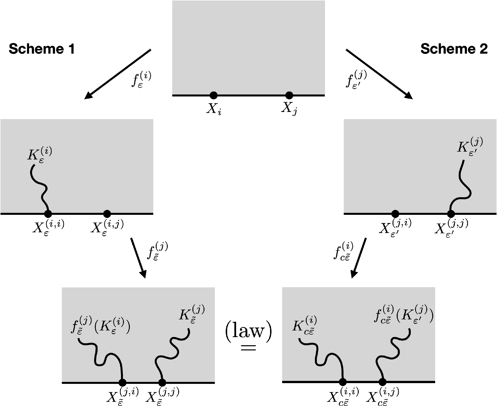
Let us fix a pair $\{i,j\}\subset\{1,\dots,N\}$. Using the backward Loewner chains introduced above, we have two schemes of generating two compact $\mathbb{H}$-hulls given an $N$-point configuration $\bm{X}=(X_{1},\dots,X_{N})\in\mathrm{Conf}_{N}(\mathbb{R})$ (see Figure 1):

Scheme 1:

Generate a compact $\mathbb{H}$-hull $K^{(i)}_{\varepsilon}$ according to the $i$-th backward SLE$(\kappa_{i},b_{i})$ $(f^{(i)}_{t}(\cdot):t\geq 0)$ starting at $\bm{X}$ up to a time $\varepsilon>0$. Next, forgetting the first compact $\mathbb{H}$-hull $K^{(i)}_{\varepsilon}$, generate the second compact $\mathbb{H}$-hull $K^{(j)}_{\tilde{\varepsilon}}$ letting the $j$-th backward SLE$(\kappa_{j},b_{j})$ $\left(f^{(j)}_{s}(\cdot):s\geq 0\right)$ starting at $\bm{X}^{(i)}_{\varepsilon}$ evolve up to a time $\tilde{\varepsilon}>0$. We also require that

$$\mathrm{hcap}\left(f^{(j)}_{\tilde{\varepsilon}}(K^{(i)}_{\varepsilon})\right)=2c\tilde{\varepsilon}$$

for a fixed $c>0$. Then, one obtains the union of two compact $\mathbb{H}$-hulls $K^{1}_{c,\tilde{\varepsilon}}:=f^{(j)}_{\tilde{\varepsilon}}(K^{(i)}_{\varepsilon})\cup K^{(j)}_{\tilde{\varepsilon}}$.

Scheme 2:

Generate a compact $\mathbb{H}$-hull $K^{(j)}_{\varepsilon^{\prime}}$ according to the $j$-th backward SLE$(\kappa_{j},b_{j})$ $\left(f^{(j)}_{s}(\cdot):s\geq 0\right)$ starting at $\bm{X}$ up to a time $\varepsilon^{\prime}>0$. Next, forgetting the first compact $\mathbb{H}$-hull $K^{(j)}_{\varepsilon^{\prime}}$, generate the second one $K^{(i)}_{c\tilde{\varepsilon}}$ letting the $i$-th backward SLE$(\kappa_{i},b_{i})$ $\left(f^{(i)}_{t}(\cdot):t\geq 0\right)$ starting at $\bm{X}^{(j)}_{\varepsilon^{\prime}}$ evolve up to a time $c\tilde{\varepsilon}>0$, where $\tilde{\varepsilon}>0$ and $c>0$ are those taken in Scheme 1. We also require that

$\displaystyle\mathrm{hcap}\left(f^{(i)}_{c\tilde{\varepsilon}}(K^{(j)}_{\varepsilon^{\prime}})\right)=2\tilde{\varepsilon}.$

Then, one obtains the union of two compact $\mathbb{H}$-hulls $K^{2}_{c,\tilde{\varepsilon}}:=K^{(i)}_{c\tilde{\varepsilon}}\cup f^{(i)}_{c\tilde{\varepsilon}}(K^{(j)}_{\varepsilon^{\prime}})$.

Notice that $\varepsilon$ and $\varepsilon^{\prime}$ are determined by $\tilde{\varepsilon}$ and $c$. In the subsequent arguments, we think of $\tilde{\varepsilon}$ and $c$ as independent parameters.

Here is the main theorem in this section.

References

• [BB03] M. Bauer and D. Bernard. Conformal field theories of stochastic Loewner evolutions. Commun. Math. Phys., 239:493–521, 2003.
• [BB04] M. Bauer and D. Bernard. Conformal transformations and the SLE partition function martingale. Ann. Henri Poincaré, 5:289–326, 2004.
• [BBK05] M. Bauer, D. Bernard, and K. Kytölä. Multiple Schramm–Loewner evolutions and statistical mechanics martingales. J. Stat. Phys., 120:1125–1163, 2005.
• [Ber16] N. Berestycki. Introduction to the Gaussian free field and Liouville quantum gravity, 2016. available at https://homepage.univie.ac.at/nathanael.berestycki/articles.html.
• [BF08] R. Bauer and R. Friedrich. On chordal and bilateral SLE in multiply connected domains. Math. Z., 258:241–265, 2008.
• [BKT18] S.-S. Byun, N.-G. Kang, and H.-J. Tak. Annulus SLE partition functions and martingale-observables, 2018. arXiv:1806.03638.
• [BPW21] V. Beffara, E. Peltola, and H. Wu. On the uniqueness of global multiple SLEs. Ann. Probab., 49:400–434, 2021.
• [BPZ84] A. A. Belavin, A. M. Polyakov, and A. B. Zamolodchikov. Infinite conformal symmetry in two-dimensional quantum field theory. Nucl. Phys. B, 241:333–380, 1984.
• [CF18] Z.-Q. Chen and M. Fukushima. Stochastic Komatu–Loewner evolutions and BMD domain constant. Stochastic Process. Appl., 128:545–594, 2018.
• [DKRV16] F. David, A. Kupiainen, R. Rhodes, and V. Vargas. Liouville quantum gravity on the Riemann sphere. Commun. Math. Phys., 342:869–907, 2016.
• [DMS14] B. Duplantier, J. Miller, and S. Sheffield. Liouville quantum gravity as a mating of trees, 2014. arXiv:1409.7055.
• [DRV16] F. David, R. Rhodes, and V. Vargas. Liouville quantum gravity on complex tori. J. Math. Phys., 57:022302, 2016.
• [DS09] B. Duplantier and S. Sheffield. Duality and Knizhnik-Polyakov-Zamokodchikov relation in Liouville quantum gravity. Phys. Rev. Lett., 102:150603, 2009.
• [DS11] B. Duplantier and S. Sheffield. Liouville quantum gravity and KPZ. Invent. Math., 185:333–393, 2011.
• [Dub06] J. Dubédat. Euler integrals for commuting SLEs. J. Stat. Phys., 123:1183–1218, 2006.
• [Dub07] J. Dubédat. Commutation relations for Schramm–Loewner evolutions. Commun. Pure and Appl. Math., LX:1792–1847, 2007.
• [Dub09] J. Dubédat. SLE and the free field: Partition functions and couplings. J. Amer. Math. Soc., 22:995–1054, 2009.
• [Dys62] F. J. Dyson. A Brownian-motion model for the eigenvalues of a random matrix. J. Math. Phys., 3:1191–1198, 1962.
• [FK15a] S. Flores and P. Kleban. A solution space for a system of null-state partial differential equations, part I. Commun. Math. Phys., 333:389–434, 2015.
• [FK15b] S. Flores and P. Kleban. A solution space for a system of null-state partial differential equations, part II. Commun. Math. Phys., 333:435–481, 2015.
• [FK15c] S. Flores and P. Kleban. A solution space for a system of null-state partial differential equations, part III. Commun. Math. Phys., 333:597–667, 2015.
• [FK15d] S. Flores and P. Kleban. A solution space for a system of null-state partial differential equations, part IV. Commun. Math. Phys., 333:669–715, 2015.
• [GMS17] E. Gwynne, J. Miller, and S. Sheffield. The Tutte embedding of the mated-CRT map converges to Liouville quantum gravity, 2017. arXiv:1705.11161.
• [Gra07] K. Graham. On multiple Schramm–Loewner evolutions. J. Stat. Mech., 2007:P03008, 2007.
• [GRV19] C. Guillarmou, R. Rhodes, and V. Vargas. Polyakov’s formulation of 2​d2d bosonic string theory. Publ. math. lHES, 130:111–185, 2019.
• [Hid80] T. Hida. Brownian Motion, volume 11 of Applications of Mathematics. Springer-Verlag New York Heidelberg Berlin, 1980.
• [HRV18] Y. Huang, R. Rhodes, and V. Vargas. Liouville quantum gravity on the unit disk. Ann. Inst. H. Poincaré Probab. Statist., 54:1694–1730, 2018.
• [IK13] K. Izyurov and Kytölä. Hadamard’s formula and couplings of SLEs with free field. Probab. Theory Relat. Fields, 155:35–69, 2013.
• [Kan07] N.-G. Kang. Boundary behavior of SLE. J. Amer. Math. Soc., 20:185–210, 2007.
• [KK20a] M. Katori and K. Koshida. Conformal welding problem, flow line problem, and multiple Schramm–Loewner evolution. J. Math. Phys., 61:083301, 2020.
• [KK20b] M. Katori and S. Koshida. Gaussian free fields coupled with multiple SLEs driven by stochastic log-gases, 2020. to appear in Adv. Stud. Pure Math.
• [KK20c] M. Katori and S. Koshida. Three phases of multiple SLE driven by non-colliding Dyson’s Brownian motions, 2020. arXiv:2011.10291.
• [KL07] M. Kozdron and G. Lawler. The configuration measure on mutually avoiding SLE paths. In Universality and Renormalization, Volume 50 of Fields Institute Communications, pages 199–224. American Mathematical Society, Providence, 2007.
• [Kna86] A. W. Knapp. Representation Theory of Semisimple Groups: An Overview Based on Examples, volume 36 of Princeton Mathematical Series. Princeton University Press, 1986.
• [Kos18] S. Koshida. Local martingales associated with Schramm–Loewner evolutions with internal symmetry. J. Math. Phys., 59:101703, 2018.
• [KP16] K. Kytölä and E. Peltola. Pure partition functions of multiple SLEs. Commun. Math. Phys., 346:237–292, 2016.
• [KP20] K. Kytölä and E. Peltola. Conformally covariant boundary correlation functions with a quantum group. J. Eur. Math. Soc., 22:55–118, 2020.
• [KRV19] A. Kupiainen, R. Rhodes, and V. Vargas. Local conformal structure of Liouville quantum gravity. Commun. Math. Phys., 371:1005–1069, 2019.
• [Law09a] G. Lawler. Partition functions, loop measure, and versions of SLE. J. Stat. Phys., 134:813–837, 2009.
• [Law09b] G. F. Lawler. Multifractal analysis of the reverse flow for the Schramm–Loewner evolution. Progress in Probability, 61:73–107, 2009.
• [Lin08] J. Lind. Hölder regularity of the SLE trace. Trans. Amer. Math. Soc., 360:3557–3578, 2008.
• [MS16a] J. Miller and S. Sheffield. Imaginary geometry I: interacting SLEs. Probab. Theory Relat. Fields, 164:553–705, 2016.
• [MS16b] J. Miller and S. Sheffield. Imaginary geometry II: reversibility of SLE(ρ1,ρ2)κ{}_{\kappa}(\rho_{1},\rho_{2}) for κ∈(0,4)\kappa\in(0,4). Ann. Prob., 44:1647–1722, 2016.
• [MS16c] J. Miller and S. Sheffield. Imaginary geometry III: reversibility of SLEκ for κ∈(4,8)\kappa\in(4,8). Ann. Math., 184:455–486, 2016.
• [MS17] J. Miller and S. Sheffield. Imaginary geometry IV: interior rays, whole-plane reversibility, and space-filling trees. Probab. Theory Relat. Fields, 169:729–869, 2017.
• [Mur20] T. Murayama. On the slit motion obeying chordal Komatu–Loewner equation with finite explision time. J. Evol. Equ., 20:233–255, 2020.
• [MZ19] B. Mackey and D. Zhan. Decomposition of backward SLE in the capacity parametrization. Stat. Prob. Lett., 146:27–35, 2019.
• [Pol81a] A. M. Polyakov. Quantum geometry of bosonic strings. Phys. Lett. B, 103:207–210, 1981.
• [Pol81b] A. M. Polyakov. Quantum geometry of fermionic strings. Phys. Lett. B, 103:211–213, 1981.
• [PW19] E. Peltola and H. Wu. Global and local multiple SLE for κ≤4\kappa\leq 4 and connection probabilities for level line of GFF. Commun. Math. Phys., 366:469–536, 2019.
• [QW18] W. Qian and W. Werner. Coupling the Gaussian free fields with free and with zero boundary conditions via common level lines. Commun. Math. Phys., 361:53–80, 2018.
• [RS05] S. Rohde and O. Schramm. Basic properties of SLE. Ann. Math., 161:883–924, 2005.
• [RS17] O. Roth and S. Schleissinger. The Schramm–Loewner equation for multiple slits. J. Anal. Math., 131:73–99, 2017.
• [RV17] R. Rhodes and V. Vargas. Gaussian multiplicative chaos and Liouville quantum gravity. In Stochastic Processes and Random Matrices: Lecture Notes of the Les Houches Summer School: Volume 104, July 2015. Oxford University Press, Oxford, 2017.
• [RZ16] S. Rohde and D. Zhan. Backward SLE and the symmetry of the welding. Probab. Theory Relat. Fields, 164:815–863, 2016.
• [Sch00] O. Schramm. Scaling limits of loop-eraced random walks and uniform spanning trees. Israel J. Math., 118:221–288, 2000.
• [She07] S. Sheffield. Gaussian free fields for mathematicians. Probab. Theory Relat. Fields, 139:521–541, 2007.
• [She16] S. Sheffield. Conformal weldings of random surfaces: SLE and the quantum gravity zipper. Ann. Prob., 44:3474–3545, 2016.
• [SS09] O. Schramm and S. Sheffield. Contour lines of the two-dimensional discrete Gaussian free field. Acta Math., 202:21–137, 2009.
• [SS13] O. Schramm and S. Sheffield. A contour line of the continuum Gaussian free field. Probab. Theory Relat. Fields, 157:47–80, 2013.
• [SW05] O. Schramm and D. B. Wilson. SLE coordinate changes. New York J. Math., 11:659–669, 2005.
• [Tak14] T. Takebe. Dispersionless BKP hierarchy and quadrant Löwner equation. SIGMA, 10:023, 2014.
• [Wer04] W. Werner. Girsanov’s transformation for SLE(κ,ρ\kappa,\rho) processes, intersection exponents and hiding exponents. Ann. Fac. Sci. Toulouse Math., 13:121–147, 2004.
• [Zha04] D. Zhan. Stochastic Loewner evolution in doubly connected domains. Probab. Theory Relat. Fields, 129:340–380, 2004.