IFT-UAM/CSIC-19-127
Shiroman Prakasha and Ritam Sinhab
a Department of Physics and Computer Science, Dayalbagh Educational Institute, Agra 282005, India
b Instituto de Fisica Teorica IFT-UAM/CSIC, Cantoblanco 28049, Madrid. Spain
We study tensor models based on symmetry groups constructed out of rank- tensors with order- interaction vertices. We refer to those tensor models for which as subchromatic. We focus most of our attention on sextic () models with maximally-single-trace interactions. We show that only three subchromatic sextic maximally-single-trace interaction vertices exist: these are the prism, the wheel (or ) and the octahedron. For theories based on these interactions we demonstrate that the set of Feynman diagrams that contribute to the free energy in the large limit are melonic and thus can be explicitly summed. In order to take into account the prism, we generalize the conventional notion of melonic diagrams slightly to include diagrams generated by a new melonic move – vertex expansion.
1 Introduction and summary
In addition to well-known adjoint/matrix model [1] and vector model large limits [2], a new large limit dominated by melonic diagrams has attracted a great deal of attention recently [3, 4, 5, 6, 7, 8, 9, 10, 11]. The melonic limit was first observed in tensor models (see [12, 13, 14, 15] for reviews), but interest in this limit grew due in large part to its appearance in the SYK model [16, 17, 18] which serves as a very educational toy model for quantum gravity [19, 20, 21, 22, 23, 24, 25, 26, 27, 28, 29, 30, 31, 32, 33, 34, 35, 36, 37, 38].
Here we seek to better understand the entire range of models for which melonic diagrams dominate. While there are important dynamical differences between the SYK model and tensor models [39, 40], tensor models provide a very natural context for understanding the diagrammatics of the melonic large limit, and its possible generalizations.
Motivated by [41, 42, 43, 44], we consider the large limit of tensor models constructed out of rank- tensors which transform in a representation of , with order-, i.e., , interactions [14]. Each index transforms in the fundamental representation of its corresponding symmetry group.
It is natural to restrict our attention to a class of interaction vertices that are maximally-single-trace (MST), first defined in [41]. (We review the definition of maximally-single-trace, and other basic features of these theories in section 2.) In the large limit, we expect that the maximally-single-trace interactions are the “most interesting” interactions, in the same sense that the tetrahedron is more interesting than the pillow and double-trace interactions for theories.11 1 To provide some justification for this expectation, we observe that all the sextic non-MST interactions in [43] can be obtained from quartic pillow and double-trace interactions via an auxiliary field. We also remark that the restriction to maximally-single-trace operators reduces the number of interactions to a much more manageable number.
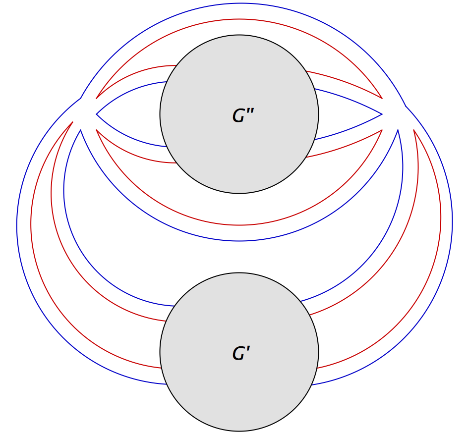
Let us discuss the large limit of theories based on such interactions. When , these theories define the familiar bifundamental model [45, 46], in the large limit, in which all planar diagrams survive. When , these theories are dominated by melonic diagrams, as recently argued in [44]. For interaction vertices with intermediate values of , i.e., , we can attempt to determine the set of diagrams which survive in the natural large limit on a case-by-case basis -- these will certainly include melonic diagrams, but additional diagrams may also contribute. An example of this is the prismatic22 2 The prismatic limit is solved by introducing an auxiliary field to rewrite the theory as a quartic tensor model with the familiar tetrahedron interaction [47, 43]. So one can argue that it is effectively still melonic. This limit can also be realized in a theory with random couplings, discussed in [48]. limit of [49, 43], where additional diagrams contribute compared to the sextic tensor model [41, 44], such as the one shown in Figure 1. Because determines the number of colours used in a multi-line ’t Hooft notation, we may also refer to as the number of “colours” of the model. We refer to models with as subchromatic33 3 An alternative name for these models is subvalent as each field vertex in the interaction graphs described in the next section have submaximal valence..

In this paper, we focus our attention on the case of with interactions. This case is the smallest non-trivial case to consider. This case is also interesting because, in addition to studying quantum mechanical models in one dimension, one can hope to define quantum field theories with interactions in dimensions.
While one might be concerned that a large number of subchromatic vertices exist for generic , the set of maximally-single-trace subchromatic vertices for turns out to be very small, as we show in section 3. For , there are two interaction vertices – namely the prism and the wheel (which also corresponds to the complete bipartite graph ) defined in [43]; and for , there is exactly one such interaction vertex, which corresponds to the graph of a regular octahedron. In section 3 we also discuss the discrete symmetries of these interactions.
In section 4 we then discuss basic features of the large limit of such theories: including the natural ’t Hooft coupling and the existence of loops passing through one or two vertices. We also define the notion of a 1-cycles and 2-cycles, which are used in subsequent analysis. These results (which mostly are a special case of a slightly more general analysis in ([41]) apply to all subchromatic maximally-single-trace interactions.
In section 5, we use the results of section 4 to characterize the set of free energy diagrams which survive in the large limit for theories based on each of the three subchromatic maximally-single-trace interactions we identified in section 3. We also consider theories based on rank- tensors that contain both prism and wheel interactions. In all cases we find the diagrams can be explicitly summed, and these theories are effectively melonic – although, the case of the prism [49, 43] might not be considered melonic in the conventional sense.
In section 5, we also argue that, in the most general “solvable” melonic theory, we expect that the set of diagrams that survive in the large limit can be generated by three types of melonic moves: replacing propagators by elementary melons, replacing propagators by elementary snails and vertex expansion. The third-move, vertex-expansion, is not present in most models previously studied; the prismatic theory is the first example of a theory for which all three types of moves are present.
Let us point out44 4 We thank Igor Klebanov for pointing out the reference [50]. that related work on sextic and theories appear in [50], where the melonic dominance of the wheel/ interaction, is discussed following [51]. We believe our work is complementary to that of [50], as we consider models, which allow for a larger number of maximally-single-trace interactions. In particular, we prove melonic dominance in the theory based on the octahedron and the theory involving both a prism and wheel interaction.
In section 6 we briefly discuss the implications for bosonic and fermionic conformal field theories based on these interactions.
In section 7, we present conclusions and several avenues for future work.
2 Preliminaries
Rank- tensor models based on fields with indices55 5 An alternative class of tensor models is defined using symmetric traceless or anti-symmetric representations of a single symmetry group [52, 53, 47]. We do not consider such theories here., , that transform under the symmetry group were introduced in [9] and studied in [11]. Here, , , and are indices that transform in the fundamental representation of each symmetry group. Similarly, theories based on rank- indices are constructed out of fields with indices that transform under the symmetry group .
The simplest theories one can define are based on a single tensor-field which is either bosonic or fermionic. Theories with quartic interactions of both types, as well as supersymmetric theories, were introduced, and subsequently studied and generalized in, e.g., [54, 55, 56, 57, 58, 59, 60, 61, 62, 63, 64, 65, 66, 67, 68, 69]. In this paper, we focus primarily on sextic interactions, for which it is natural to consider bosonic theories in dimensions, and fermionic theories in (i.e., quantum mechanical models).
A variety of interactions for tensor models exist, which are obtained by contracting the indices in various ways. For example, the wheel interaction [43] is represented by the following interaction term:
| (2.1) |
We divide the coupling constant by because that is the size of the automorphism symmetry group of this interaction, as discussed in section 3.2.
One way of drawing Feynman diagrams for the rank- tensors is via a triple-line notation that is a straightforward generalization of ’t Hooft’s double-line notation. Each propagator is represented by three coloured lines, with different colours representing the different indices , and ; as shown in Figure 2(a). The wheel interaction vertex is represented by the vertex shown in Figure 2(b).
A two-loop correction to the propagator is shown in Figure 3. As we will show in section 4, the natural ’t Hooft coupling for the wheel is . In the large limit, with the ’t Hooft coupling fixed, this is a leading-order diagram proportional to . This diagram is also an elementary melon. In melonic theories, any leading-order diagrams can be obtained by repeatedly replacing propagators by elementary melons. We will discuss this in more detail in section 5.2.


For the purpose of systematically enumerating all possible interactions, it is more convenient to represent interactions by an interaction graph, as shown in Figure 4. Each vertex in the interaction graph represents a field. Each symmetry group corresponds to a different colour, and coloured edges denote contractions of the corresponding indices. We will refer to the vertices of the interaction graph as field-vertices, or simply fields, to avoid confusion with “interaction vertices” in Feynman diagrams.

It is convenient to label the fields-vertices of an interaction graph by , , …; where represent the momenta of each field, and are “dummy indices”, as can be seen from the momentum-space representation of the vertex:
| (2.2) |
Two labelled interaction graphs correspond to the same interaction if they can be made identical by a permutation of outgoing-field labels.
Each interaction will be presented with a conventional set of labels for its fields, such as the labels given in Figure 4. One advantage of using these labels is that one can unambiguously represent Feynman diagrams in single-line notation. The elementary melon of Figure 3 can also be represented as a single-line Feynman diagram, using field-labels, as shown in Figure 5.

An interaction graph representing an interaction of rank- tensors will involve edges of different colours. Given a multi-line interaction graph with colours, one can remove all lines of a given colour, to obtain an interaction graph with colours. For example, in Figure 6, if we forget the green edges in the graph on the left, we obtain the -colour interaction graph on the right. We call this process “forgetting” a colour. Given an interaction graph, it is convenient to sometimes forget all but colours. We call the resulting interaction graph a two-colour subgraph.

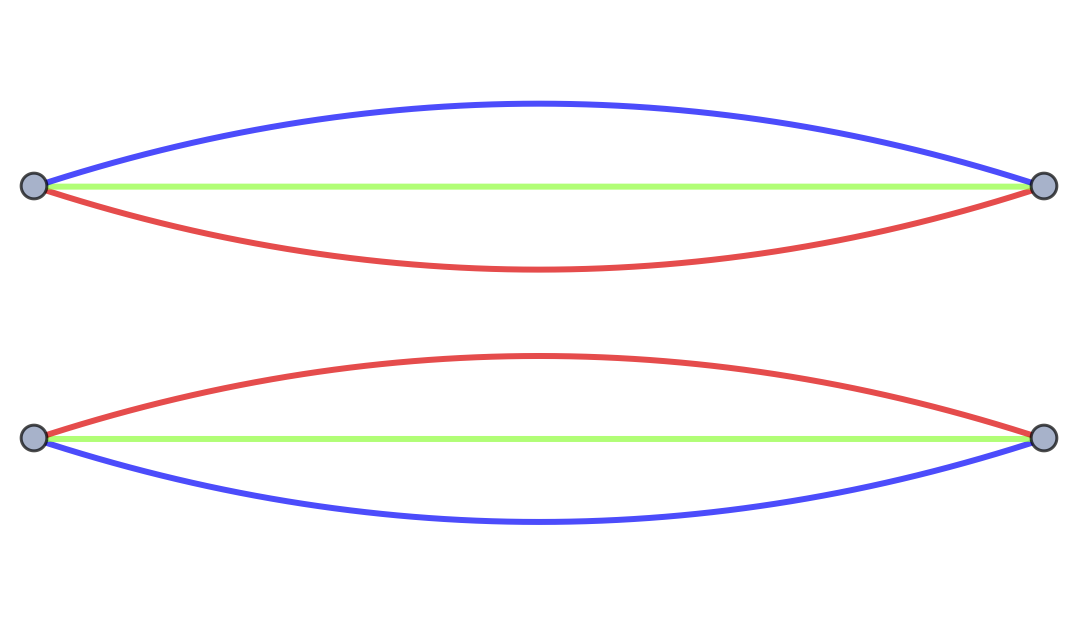
We say that an interaction vertex is single-trace if it is represented by a connected interaction graph. An interaction is maximally-single-trace (MST) if all its two-colour subgraphs are single-trace [41]. As an example, representatives for all the quartic interaction vertices are pictured in Figure 7. The tetrahedron vertex is maximally-single-trace; the pillow interaction is single-trace, but not maximally-single-trace; and the double-trace interaction is not single-trace.


3 Sextic maximally-single-trace interactions
The only quartic maximally-single-trace interaction is the tetrahedron. In this section, we enumerate all the sextic maximally-single-trace interactions and discuss their symmetries. Related discussion for tensor models of maximal rank appears in [41, 44].
3.1 Constructing all sextic maximally-single-trace interactions
Here we construct all maximally-single-trace sextic vertices for subchromatic tensor models. For , there is one MST vertex, the usual single-trace interaction. Note that this must take form of a connected cyclic graph with edges of alternating colours, which we take to be red and green, as shown in Figure 8.

Let us now consider the MST interactions. Note that upon forgetting one colour from an MST interaction graph, we are left with the cyclic graph. To construct an MST interaction, we need to add three blue edges to the red-green cyclic graph of Figure 8, such that the red-blue and green-blue subgraphs are also cyclic graphs. Note that, if we use a blue edge to connect two vertices that were already connected by a green edge, then the blue-green subgraph will consist of two or more disconnected components – hence there are not very many possibilities to consider for the locations of the blue edges. One can explicitly check all possibilities to see that there are exactly two ways to add blue edges which result in an MST interaction – these correspond to the prism and the wheel of [43] shown in Figures 9 and 10.
The wheel interaction graph is also known as (the complete bipartite graph consisting of two sets of 3 vertices) in the graph theory literature, which is one of the two simplest non-planar graphs.


We will refer to the three colours of the interactions as .
Let us now consider the case of . When any one colour is forgotten, the MST interaction must reduce to a prism or wheel. As before, we consider all ways of adding (three) yellow edges to the prism or the wheel, such that the resulting interaction is MST. We find that there is no way of adding yellow edges to the wheel interaction while preserving the MST property; and there is exactly one way to add yellow edges to the prism interaction that preserves MST. Hence there is a unique MST vertex, depicted in Figure 11. We will refer to the four colours of the interaction as . If one redraws this graph in three-dimensions, one can see that it corresponds to a regular octahedron.66 6 We thank Igor Klebanov and Martin Roček for pointing this out to us. Another name we used for this interaction is the double-prism, as both the and subgraphs of this interaction are prism interactions. Hence we refer to this as the octahedron interaction.


It turns out that one can add a colour to the MST vertex while preserving the MST property. This gives rise to the unique MST vertex. This interaction contains the maximal number of colours for a sextic vertex, and gives rise to a traditionally melonic large limit, as discussed in [41, 44].
This recursive procedure of adding colours to subchromatic graphs can be repeated to enumerate all MST interactions for larger values of as well.
3.2 Automorphism and colour permutation symmetry
All of the three MST interactions identified above have a discrete symmetry – they are symmetric under permutation of the symmetry groups. In terms of the graphical representation of interactions, this is a discrete symmetry under permutation of the various colours in an interaction graph. The interactions may also posses a non-trivial automorphism symmetry group.
We represent symmetry operations by permutations of the field-vertices in the labelled interaction graph. If a field permutation gives rise to a labelled interaction graph isomorphic to the original, is an element of the automorphism group of the interaction vertex. If a field permutation gives rise to a labelled interaction graph isomorphic to the original graph, up to a permutation of colours, then is an element of the colour permutation symmetry group.
In order to show that an interaction is symmetric under all colour permutations, we require that, for each permutation of colours (i.e., relabelling of edges), there is a permutation of field-labels that leaves the labelled interaction graph unchanged. For rank-three interactions, we need to check that all colour permutations which are generated by the two generators and , correspond to field-label permutations. For the rank-four interaction, the colour permutation group has 3 generators: , , and , and we need to verify that each of these generators corresponds to a permutation of field-labels.
Let us first consider the prism. We draw the prism interaction in two different ways in Figure 12, from which we can see that is equivalent to the field-vertex permutation , and is equivalent to the field-vertex permutation . We also see that the field-vertex permutation leaves all colours the same. Hence, the prism interaction should conventionally come with a factor of in the Lagrangian.


We next consider the wheel (or ) interaction. We draw the wheel in two different ways in Figure 13, from which we can see that is equivalent to the field-vertex permutation , and is equivalent to the field-vertex permutation . We see that the field-vertex permutations and leave all colours the same. Hence, the wheel (or ) interaction should conventionally come with a factor of in the Lagrangian.


Finally, we consider the octahedron. We draw the octahedron in three different ways in Figure 14, from which we can see that is equivalent to the field-vertex permutation , , and . There is no field-vertex permutation that leaves all colours the same, so the interaction comes with a factor of in the Lagrangian.


Let us conclude this section with the observation that, if the automorphism symmetry group includes a field-vertex permutation that is odd, then, in a theory of Majorana fermions, the 1-dimensional fermionic interaction term based on that interaction vanishes due to anti-commutation of Grassmann variables.
In particular, as observed in [40], for the wheel:
| (3.1) | |||||
| (3.2) | |||||
| (3.3) |
In the second line, we applied the field permutation . In the third line, because this is an automorphism, we are able to relabel the dummy indices , and (via: , ) to undo this permutation. Similarly, for the prism:
| (3.4) | |||||
| (3.5) | |||||
| (3.6) |
These arguments do not apply to complex fermions.77 7 We thank Igor Klebanov for discussions on this point.
Let us also remark that, if we would like to define an theory with complex fields, and promote all the symmetry groups to , then we require the interaction graph to be bipartite. The wheel is bipartite, but the prism, the octahedron and the unique sextic MST interaction of [41, 44] are not bipartite. If we wish to promote some, but not all, of the symmetry groups to , this restriction does not apply.
In all cases, real bosonic versions of these theories can be defined, and can be thought of as special cases of the general sextic bosonic theory studied perturbatively in [70].
4 Large limit of subchromatic maximally-single-trace interactions
We now consider the large limit of the maximally-single-trace interaction vertices defined in the previous section. In this section we present results for an arbitrary maximally-single-trace interaction of any order . We follow the approach outlined in [11]. The results of this section are a special case of a more general analysis of the large limit of maximally-single-trace interactions given in [41].
4.1 Large scaling of coupling constants
Let us first determine the natural scaling of the coupling constant with , in the large limit, for an order- maximally-single-trace interaction with indices.
Consider a connected Feynman diagram with no external edges, i.e., one that contributes to the free energy of our theory. As shown in the previous sections, Feynman diagrams for fields based on rank- tensors can be drawn in a multi-line notation, using different colours. If we take any such diagram, and erase all but two of the colours, we obtain a two-colour fat graph, or simply fat graph. Since our multi-line propagator contains colours, we can generate fat graphs – one for each pair of colours. We shall use the index , where , to label each of these fat graphs. We denote the number of loops for each fat graph by . Then, summing over all such pairs of indices, we obtain,
| (4.1) |
where is the total number of loops in the multi-line Feynman diagram and determines the power of .
Because our interaction vertices are maximally-single-trace, each fat graph will consist of a single connected component. The Euler equation for each can be written as,
| (4.2) |
where and refer to the number of vertices and edges in the graph (which are the same for all fat graphs) and is the genus of the fat graph labelled by . We define maximal Feynman diagrams to be those with the largest for a given . From the above formula, we see that maximal Feynman diagrams satisfy , i.e., maximal Feynman diagrams are those diagrams that give rise to only planar fat graphs.
Since our vertices are order-, we have . Placing this into the above equation, we obtain,
| (4.3) |
Now, summing over all , we get
| (4.4) | ||||
which imply,
| (4.5) |
Maximal Feynman diagrams saturate the above bound, and must satisfy:
| (4.6) |
This relation tells us that we should define the large limit while keeping the ’t Hooft coupling
| (4.7) |
fixed. (This is essentially the same as Equation (3.37) of [41].) Then, the free energy scales with as,
| (4.8) |
4.2 Existence of a loop passing through one or two vertices
We now show that any connected maximal diagram contributing to the free energy contains a loop passing through exactly one vertex or a loop passing through exactly two vertices.
Let us define to be the number of loops passing through vertices [11]. Clearly,
| (4.9) |
Also, by considering the total number of coloured lines passing through a vertex in the multi-line notation, one can see that:
| (4.10) |
Combining (4.9) and (4.10), and eliminating using (4.6), we obtain
| (4.11) |
When , one can separate the terms and from the sum, to obtain the following inequality:
| (4.12) |
The above analysis assumed that the number of interaction vertices was greater than or equal to . The trivial free-energy diagram which contains no interaction vertices, is also maximal. Thus, we have the following result:
Theorem 1.
Any maximal, non-trivial, multi-line Feynman diagram contributing to the free energy contains at least one loop passing through one vertex, or one loop passing through two vertices.
4.3 1-cycles and 2-cycles
In our subsequent analysis, it will be convenient to distinguish between single-line Feynman diagrams and multi-line Feynman diagrams. Each single-line Feynman diagram (constructed from labelled interaction vertices) corresponds to a multi-line Feynman diagram and vice-versa. (There may be multiple ways of labeling the interaction vertices in the single-line diagram corresponding to a given multi-line diagram, due to the automorphism symmetry of each interaction, but this does not affect our discussion.)
A single line Feynman diagram contributing to the free energy is a graph, i.e. a collection of vertices and edges. A walk of length in a graph is defined to be an ordered sequence of edges , that joins a sequence of vertices . A closed walk is a walk that starts and ends on the same vertex, i.e., . Let us define an -cycle as a closed walk of length , such that no edge or vertex is repeated, other than the starting vertex which is the same as the end vertex. This is the usual notion of a cycle in graph theory.
In the previous subsection, we defined as the number of loops passing through vertices in a multi-line Feynman diagram. Any loop passing through vertices in a multi-line Feynman diagram induces a closed walk of length , with distinct edges, in the corresponding single-line Feynman diagram. (Of course, the converse is not be true – a closed walk in the single line Feynman diagram need not correspond to a loop in the multi-line Feynman diagram.) Note that a closed walk of length is necessarily a -cycle. Note also that a closed walk of length with distinct edges is either a 2-cycle, or passes through the same vertex twice, in which case it is the union of two (possibly identical) 1-cycles.
Theorem 1 of the previous subsection therefore implies the following theorem.
Theorem 2.
Any maximal, non-trivial, single-line Feynman diagram contributing to the free energy must contain at least one 1-cycle, or at least one 2-cycle.
Theorem 2 is slightly weaker than Theorem 1 of the previous subsection, but it will be more convenient to apply Theorem 2 in the subsequent analysis.
While Feynman diagrams containing 1-cycles may be unphysical, we include them in the analysis below, in order to obtain purely combinatorial constraints on the diagrams that contribute in the large limit.
5 Melonic dominance of subchromatic interaction vertices
Here, we focus our attention on theories based on the sextic MST interactions obtained in section 3. We can define a theory with , to contain a wheel interaction, a prism interaction, or both. We can also define a theory with based on the octahedron interaction. The theory for was discussed in [41, 44] so we do not discuss it here.
5.1 General strategy
We wish to explicitly characterize and generate all the maximal Feynman diagrams that contribute to the free energy in any of the above theories. Our arguments are inspired by [41, 71, 44].
Our strategy is as follows. In the previous section, we demonstrated that any Feynman diagram, drawn in single-line notation, contributing to the free energy that survives in the large limit must either:
- 1.
Contain no vertices, in which case it is just the zeroth-order diagram.
- 2.
Contain at least one 1-cycle.
- 3.
Contain at least one 2-cycle.
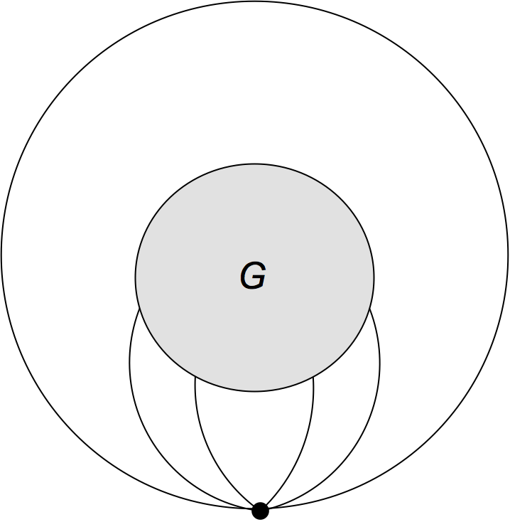
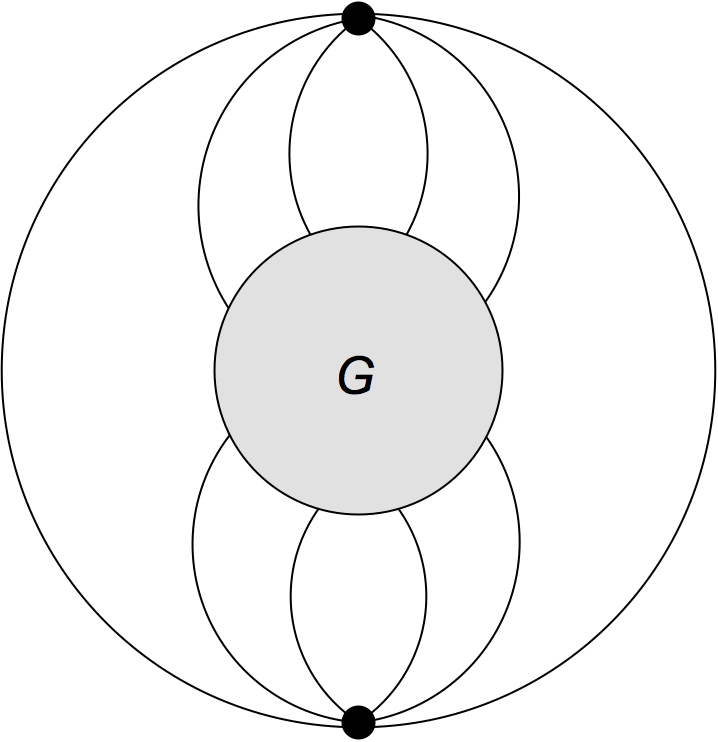
These cases are illustrated in Figure 15. Note also that a 2-cycle cannot pass through the same vertex twice by definition, so we do not need to treat this case separately. (A loop passing through the same vertex twice in the multi-line Feynman diagram would give rise to a 1-cycle in the single-line Feynman diagram.)
To enumerate all the maximal Feynman diagrams contributing to the free energy, we need to enumerate all the inequivalent free energy diagrams containing a 1-cycle or a 2-cycle. (In a slight abuse of terminology, we refer to these as inequivalent 1-cycles or 2-cycles.) For each inequivalent 1-cycle and 2-cycle, we draw each of its fat graphs, and impose the restriction that each fat graph is planar.
When we draw a fat graph corresponding to a particular pair of colours, we must arrange the outgoing lines from each interaction vertex in a particular cyclic order, for the fat graph to be manifestly planar. For example, consider the wheel interaction, shown in Figure 22. If we draw a blue red fat-graph, we must arrange the outgoing lines of each interaction vertex in the cyclic order (or ). If we instead draw a red-green fat-graph, we must arrange the outgoing lines of each interaction vertex in the cyclic order (or ).
For a given pair of colours, the requirement of fat-graph planarity might rule out a particular 2-cycle entirely, as is the case for the 2-cycle shown in Figure 16 which contains an odd number of twists. Alternatively, the requirement of fat-graph planarity may “divide” the subgraph into two smaller disconnected components and as shown in Figure 17.

Suppose, for each inequivalent 1-cycle and 2-cycle consistent with fat-graph planarity, the requirement of fat-graph-planarity splits the subgraphs of Figure 15(b) and 15(c) into disconnected components, as shown in Figure 18. Crucially, each of these sub-graphs in Figure 18 contains only two external edges. This fact allows us to use a cutting and sewing argument to isolate the graphs , as illustrated in Figure 19. Each of the cut-and-sewn subgraphs defines a maximal Feynman diagram contributing to the free energy, with fewer interaction vertices than the original diagram. The arguments of this section apply to the cut-and-sewn subgraph as well, so we obtain a recursive enumeration of all the Feynman diagrams contributing to the free energy.


5.2 Melonic diagrams
We now discuss the recursive enumeration of the diagrams that contribute in the large limit, following [41] with some generalizations.
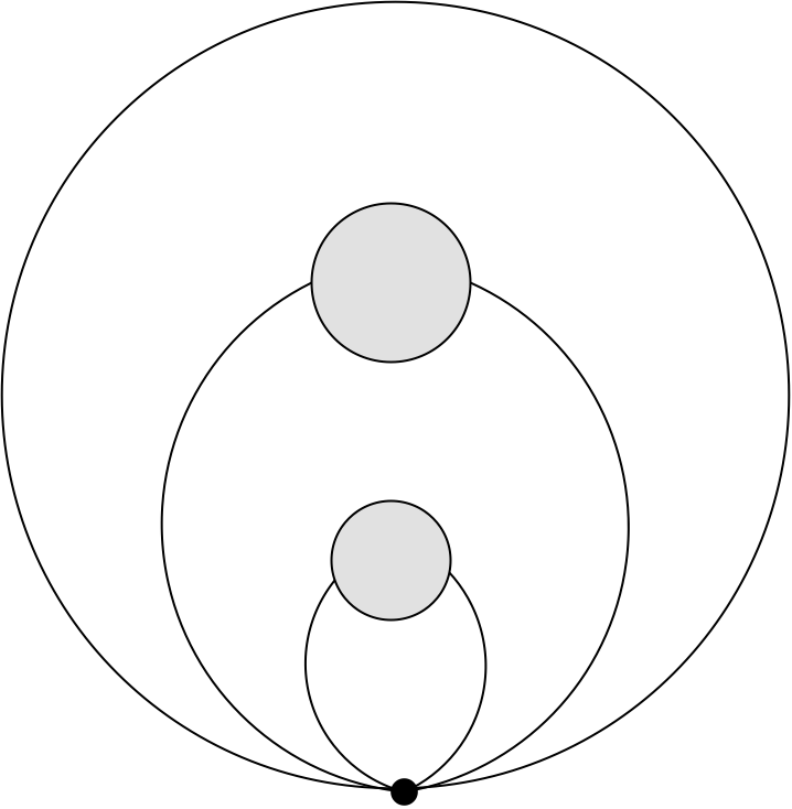
The set of maximally free energy diagrams enumerated by this recursive procedure above can typically also be obtained starting from the -cycle by repeatedly replacing propagators by elementary snails or elementary melons as shown in Figure 20.


The set of all elementary melons can be obtained from the list of maximal free-energy graphs containing a -cycle: we first replace all subgraphs (shaded blobs) by free propagators, and then cut any one of the edges open to obtain an elementary melon such as the one shown in Figure 20. The set of all elementary snails can be obtained from the list of maximal free energy graphs containing a -cycle in a similar manner.
The act of replacing a propagator by an elementary snail or elementary melon is called a melonic move. More generally, we may consider a theory with additional melonic moves. Given a set of melonic moves, we define the set of melonic diagrams to be the set of diagrams that can be generated by making an arbitrary number of melonic moves on the -cycle.
After identifying the complete set of melonic moves, it is straightforward to check that all melonic diagrams are maximal. For instance, using the elementary melon defined for the wheel interaction, it is easy to check that if the act of replacing a propagator by an elementary melon causes and . We also have a similar result for the elementary snail. Hence, if one acts on a maximal Feynman diagram with either of the two above elementary melonic moves, the relation (4.6) is preserved.
However, we would like to know if the converse is true for a given model, i.e., are all maximal diagrams in a given theory melonic? This requires us to carry out the analysis outlined in the previous subsection, which also enumerates the complete set of melonic moves for a given model. We summarize this argument here:
- 1.
We argued that any free energy diagram must take one of the three forms shown in Figure 15. For each of the interaction vertices shown in Figure 15, we must consider all possible ways of labeling the outgoing lines. There are a large but finite number of ways to do this. For the interactions we study in this paper, many labellings are equivalent to each other via the colour permutation and automorphisms described in section 3.2, which reduces the number of cases we need to check. We refer to this stage of the argument as “enumerating all inequivalent 1-cycles and 2-cycles”.
- 2.
For each inequivalent 1-cycle or 2-cycle, we then impose the constraint of planarity on each of the two-colour fat graphs, as illustrated in Figures 16 and 17. These constraints translate into restrictions on the subgraphs shown in Figure 15. We refer to this stage of the argument as “imposing fat-graph planarity”.
- 3.
By tracing the index contractions of lines flowing out of each subgraph, we attempt to replace the original Feynman diagram containing the subgraph with a simpler Feynman diagram . We must be able to argue that the original Feynman diagram is maximal if and only if the simpler Feynman diagram is maximal. We refer to this stage of the argument, depicted in Figures 18 and 19, as “cutting and sewing”. (Here, we say is “simpler” than if it contains fewer interaction vertices.)
- 4.
The inverse of the “cutting and sewing” argument, i.e., replacing with , defines a melonic move. If we can find a “cutting and sewing” argument for each inequivalent 1-cycle and 2-cycle, then we can enumerate the entire list of melonic moves that apply to our model. We can also conclude that all maximal diagrams can be obtained from the action of melonic moves on simpler diagrams. Therefore, the model is, in principle, solvable in the large limit. We refer to this stage of the argument as “collecting all melonic moves”.
For any given model, this 4-stage procedure may lead to three possible outcomes:
- 1.
If the set of melonic moves so obtained involve only replacing propagators by elementary melons or elementary snails, as shown in Figure 20, the model is melonic in the conventional sense.
- 2.
- 3.
If the cutting and sewing argument fails for any 1-cycle or 2-cycle, (i.e., we cannot find a simpler to replace for some labelling of the vertices) then the theory may not be solvable in the large limit. (This is the case, for instance, when .)
We propose that any theory for which case 1 or 2 applies, should be considered as a generalized melonic theory, even if it is not conventionally melonic.
We can ask what are the most general set of melonic moves possible? Note that, contains 1 or 2 interaction vertices (excluding interaction vertices in subgraphs). contains at most 1 interaction vertex (excluding interaction vertices in subgraphs). Therefore there are three types of melonic moves possible in our generalized notion of a melonic theory,
- 1.
Replacing a diagram containing 0 interaction vertices (i.e., a propagator) with a diagram containing 1 interaction vertex, (e.g., an elementary snail).
- 2.
Replacing a diagram containing 0 interaction vertices with a diagram containing 2 interaction vertices, (e.g., an elementary melon).
- 3.
Replacing a diagram containing 1 interaction vertex with a diagram containing 2 interaction vertices, (i.e., vertex expansion).
Most well-known melonic theories only involve moves of the second type, or possibly of the first two types. However, we will see below that the prismatic model is an example of a theory that contains a move of the third type.
For conventionally melonic theories, the melonic moves directly translate into the equation for the exact propagator shown in Figure 21. The snails may or may not be present depending on the interaction. As mentioned earlier, the snails are tadpoles, and would formally vanish in a quantum field theory due to dimensional regularization.
Let us conclude this section with the caveat that, while it is straightforward to obtain the Schwinger-Dyson equation for the exact propagator, if one wants to actually evaluate the free energy, one must also include the symmetry factors for each of these diagrams. As one can see from the diagrammatic expansion for the free energy in a vector model, e.g., [72], these factors are generally non-trivial to obtain.

5.3 Wheel (or ) interaction
In this section we demonstrate the melonic dominance of the wheel vertex, according to the general recipe above. The wheel vertex is shown in Figure 22, along with its three two-colour fat vertices.


Diagrams containing a 2-cycle
A 2-cycle is specified by two Wick contractions. We label the two interaction vertices and ; each Wick contraction must include one field from each interaction vertex. We thus specify the two Wick contractions that define the 2-cycle in the following notation: , where , , , and are integers between and corresponding to the field labels given in the labelled interaction graph of Figure 10. The notation means that field from the left interaction vertex labelled by the number in the labelled interaction graph is contracted with the field labelled by the number from the right interaction vertex [44].
A priori there are a large number of different 2-cycles that are possible. However, using the automorphism and colour permutation symmetries of the wheel interaction, we can reduce the total number of inequivalent 2-cycles to a very manageable number. The idea behind this is that if a particular 2-cycle induces only planar fat graphs, then the same must be true for any other 2-cycle obtained by a permutation of colours. Hence we do not need to check all different 2-cycles: we only need to check the subset of 2-cycles whose orbit under the colour permutation (and automorphism) symmetry group covers all 2-cycles. This is an elementary exercise in group theory, which, for the sake of clarity and completeness we spell out explicitly in the appendix.
As shown in the appendix, the inequivalent 2-cycles are
- 1.
,
- 2.
,
where or , and or .
Not all these 2-cycles give rise to planar fat-graphs. If is odd, or if is even, one can check that the red-green fat graph arising from this 2-cycle contains an odd number of twists, and hence is non-planar. Hence there are only four different 2-cycles to consider.
Let us first consider the 2-cycle . The three fat graphs for this 2-cycle are shown in Figure 23. Using these constraints we have two possibilities for the form of a free-energy diagram containing this 2-cycle, shown in Figure 24.


Let us next consider the 2-cycle . The three fat graphs for this 2-cycle are shown in Figure 26. Using these constraints we have one possibility for the form of a free-energy diagram containing this 2-cycle, also depicted in Figure 26.
We carry out a similar analysis for the 2-cycle ; the form of any free-energy diagram consistent with planarity of fat-graphs is shown in Figure 25.


For the 2-cycle , we find there is no way to satisfy the constraints that all fat-graphs be planar.
Diagrams containing a 1-cycle
A 1-cycle is formed by contracting two fields from the same interaction vertex, which we denote as . Using the automorphism symmetry of the wheel interaction, we can always choose the first field . Via colour permutation symmetry, the second field can be chosen to be or . There are thus two inequivalent 1-cycles: and .
The 1-cycle results in a non-planar red-green fat graph, so is non-maximal. The 1-cycle is constrained by planarity of the red-blue fat graph to be of the form in Figure 27.

Melonic Moves
From the inequivalent -cycles and -cycles above, we can extract the elementary melon and elementary snail shown in Figure 28.

5.4 Octahedron interaction
Let us now consider the octahedron. (We present this case before the prism, because it also gives rise to a conventional melonic limit.) Its fat vertices are pictured in Figure 29.


Diagrams containing a 1-cycle
One can check that, for the octahedron, there is no way of forming a 1-cycle such that all six fat-graphs are planar. Hence elementary snails are ruled out on purely combinatorial grounds.
Diagrams containing a 2-cycle
Let us enumerate all inequivalent 2-cycles: passing through two octahedron interaction vertices.
The octahedron has no automorphism symmetry. However, we can use the colour permutation symmetry to reduce the number of cases one has to check to ensure all fat-graphs are planar.
By permuting the colours in the Feynman diagram, any 2-cycle can be mapped to one in which . This procedure does not use all the colour permutation symmetry, as the permutation corresponds to the field-vertex permutation , which leaves the choice of invariant. In case was chosen to be or , one could use the colour permutation to map it to an equivalent diagram where . We can thus set or . If , then the colour permutation symmetry still remains at our disposal to set or . Finally, if , the unused colour permutation symmetry can be used to set or .
The inequivalent 2-cycles can thus be taken as:
- 1.
- 2.
- 3.
- 4.
- 5.
- 6.
Unless , , , one of the two-colour fat-graphs will contain an odd number of twists. Cases 2 and 3 also give rise to fat graphs with an odd number of twists, so these cases are also ruled out. We finally have only four possibly-planar inequivalent 2-cycles, which are:
- •
- •
- •
- •
Drawing all fat-graphs for each 2-cycle as we did for the wheel, we obtain the following results. We find that any free energy diagram containing the 2-cycle , or , gives rise to at least one non-planar fat graphs. Hence any free-energy diagram containing these cycles is non-maximal.
Next we consider free-energy diagrams containing the 2-cycle . Requiring all fat graphs to be planar gives rise to a free energy diagram of the form shown in Figure 30. An identical result holds for free-energy diagrams containing the 2-cycle .

Melonic moves
Putting all these results together, we find that this model is melonic in the conventional sense. All diagrams can be generated by replacing propagators by the elementary melon shown below in Figure 31. There is no elementary snail, unlike the case of the wheel.
5.5 Prism interaction
Let us now consider the prism interaction. The prism interaction and its two-colour fat vertices, are shown in Figure 32. In [49, 43], it was shown that the leading order diagrams arising from the prism interaction can be explicitly summed by using an auxiliary field to convert it into a quartic tetrahedron interaction.
However, if we do not introduce this auxiliary field, and simply draw Feynman diagrams using the sextic prism vertex, we find that there are maximal diagrams which are not melonic in the sextic sense. In other words, the set of maximal Feynman diagrams in the prismatic theory includes diagrams that would not be maximal in a conventional melonic theory, such as a theory based on the octahedron or a theory based on the maximally-single-trace interaction studied in [41, 44]. An example of such a diagram is shown in Figure 1.
Because the prism interaction gives rise to a large limit that is not conventionally melonic in this sense, it is interesting to see how the method of analysis given above can be modified to characterize all maximal diagrams.

Diagrams containing a 1-cycle
One can check that the only maximal free energy diagram containing a 1-cycle is , or its colour permutations. It takes the form shown in Figure 33.

Diagrams containing a 2-cycle
Consider two prism interaction vertices, one denoted by and the other . As before, we specify a 2-cycle, by the following contractions: .
We can choose using the automorphism of the first interaction vertex and the colour permutation symmetry. The automorphism symmetry of the second vertex and the residual colour permutation symmetry group can be used to choose or . If the residual colour permutation symmetry can be used to set or Thus, we have the following inequivalent 2-cycles,
- 1.
- 2.
where .
After removing those which give rise to fat-graphs with an odd-number of twists, we find the allowed 2-cycles are:
- 1.
- 2.
- 3.
- 4.
- 5.
Let us look at the structure of the constraints imposed by requiring fat graphs planarity for free-energy diagrams containing these cycles.
First, one can check that free energy diagrams containing the -cycles and always give rise to a non-planar fat graph, and are hence non-maximal.
Next consider the 2-cycle . Planarity of the fat graphs restricts any free energy diagram containing this cycle to be of the form shown in Figure 34.
We then consider the case . Free energy diagrams containing this 2-cycle (not pictured) are either a conventional melonic diagram, or a double-snail.


We finally consider free energy diagrams containing the 2-cycle . We observe that the requirement of planar fat subgraphs, does not split the subgraph into 4 disconnected components, as it did for the other cases. Instead, as shown in Fig 35, we are left with one subgraph with two external edges and one subgraph with six external edges.


New melonic move
In order to obtain a recursive enumeration of diagrams in this case, we need to adapt the cutting and sewing rules given earlier to the subgraph containing 6 external lines. We show how this is done in Figure 36. By carefully following the index contractions, one can check that the diagram on the left in Figure 36 is maximal if and only if the diagram on the right is maximal.


The diagram on the right in Figure 36 (which contains one fewer interaction vertex than the original diagram) is a free energy graph that contains at least one vertex, so it must take one of the forms enumerated in the previous section. By cutting out one prism interaction vertex from any of these forms, we can determine all the possibilities for subgraph in Figure 36. We have thus formally obtained a recursive procedure for generating all free-energy graphs.
In practice, it is helpful to translate this enumeration into the language of melonic-moves. We note that, in addition to the usual melonic move of replacing a propagator by an elementary snail or melon, Figure 36 requires us to introduce an additional move. From the possibility that the subgraph could be obtained from cutting out one interaction vertex from the non-melonic 2-cycle of Figure 35 itself, we obtain the new “vertex-expansion” move of replacing an interaction vertex by two-interaction vertices contracted in a particular way, as shown in Figure 37.88 8 We would like to thank Adrian Tanasa and Victor Nador for discussions on this point This vertex expansion move can be thought of as the “inverse” of the cutting and sewing rule of Figure 36. All maximal diagrams can be produced by application of this melonic move, along with the melonic moves of replacing a propagator by an elementary melon or elementary snail.
One can also check that under this move, and , so the maximality condition (4.6) is preserved, so all diagrams produced by this move are maximal.
It is easy to check that the diagrams produced by this melonic move are equivalent to those produced by the auxiliary field in [49, 43].

5.6 Theory with both a prism and wheel
Let us also consider a theory with both maximally-single-trace interactions, the prism and wheel. The allowed 1-cycles remain those from the prism and wheel theories respectively, but the 2-cycles now also include the possibility of a closed path passing through one wheel vertex and one prism vertex. We analyze this case now.
Let us assume the vertex is a prism and the vertex is a wheel. As shown in the appendix, the inequivalent 2-cycles are:
- 1.
,
- 2.
,
- 3.
,
- 4.
,
- 5.
.
All of the 2-cycles of the form 1, 2 and 4 contain an odd number of twists in one of the two-colour fat graphs, and are non-maximal.
Case 3 and Case 5 allow for a double snail. There are no other possibilities. In particular there is no new elementary melon containing both a wheel and a prism vertex, and the elementary moves of the prism theory and the wheel theory generate all Feynman diagrams.
6 Comments on field-theories based on these interactions
In this section we discuss specific realizations of these theories. Let us focus our attention on obtaining IR fixed points with physics similar to the SYK model. A list of theories involving a single, real rank- tensor field that can be solved via the analysis given above includes:
- 1.
A quantum-mechanical theory of rank- Majorana fermions based on the octahedron interaction.
- 2.
A dimensional theory of rank- real bosons dominated by the octahedron interaction.
- 3.
A dimensional theory of rank- real bosons dominated by the wheel interaction.
- 4.
A dimensional theory of rank- real bosons dominated by the prism interaction.
- 5.
A dimensional theory of rank- real bosons dominated by both the wheel and the prism interaction.
All the bosonic theories face difficulties, such as a complex spectrum, in higher dimensions, with the possible exception of the last case that has not yet been carefully studied.[48, 49, 43]
We have argued that theory of real, rank-, fermionic tensors based on the octahedron is dominated by melonic diagrams. Hence we expect its large saddle point solution will proceed exactly along the lines of [44], and in particular we expect essentially the same spectrum as the SYK model. It might be interesting to study the theory more carefully, including numerical studies to compare its behaviour at finite to the rank- melonic tensor model studied in [41, 44] or other models [73, 74, 75, 76, 77, 78], but we do not do this here.
The bosonic version of this theory, which can be defined for , also dominated by melonic diagrams. Its large saddle point solution will proceed exactly along the lines of the bosonic theories discussed in [54]. We illustrate this explicitly in subsection 6.1 below.
For the large solution of the theory of rank- real bosons with a wheel interaction, the only difference from the traditional melonic theory is the presence of the elementary snail. This elementary snail is a tadpole, so it does not appear to affect the results of the Schwinger-Dyson equation for the exact propagator. We, therefore, again expect the large solution to again proceed along the lines of the bosonic tensor models discussed in [54]. However, one slightly novel feature of the wheel interaction is that it allows us to define a theory of complex bosons with symmetry group, as its interaction graph is bi-partite.
The large solution to the theory of rank- bosons with a prism interaction was discussed in [49, 43]. We now have the possibility of solving for the large limit of a theory of rank- bosons with both the wheel and prism interactions. We leave this for future work.
6.1 Real sextic bosonic theories with melonic dominance
Let us first consider the rank- bosonic theory with the octahedron interaction. The Lagrangian for this theory is:
| (6.1) |
The ’t Hooft coupling for this theory is .
To write down the gap equation, we need to carefully count all the melonic Wick contractions that take the form of the elementary melon in Figure 31. Let us denote this number by . Here . The gap equation in the strong coupling limit takes the form:
| (6.2) |
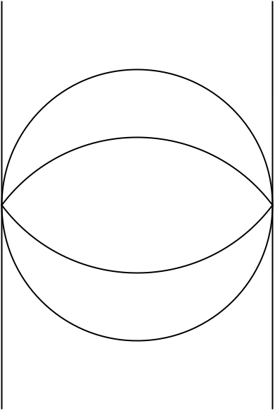
Let us now write the integration kernel:
| (6.3) |
where is the number of melonic Wick contractions of the form given in Figure 38. Clearly, for any melonic Wick contraction that takes the form of the elementary melon, one simply has to choose an internal line to cut, in order to obtain a melonic Wick contraction for the kernel, so , where in our case. If we now absorb into , our Schwinger-Dyson equations become:
| (6.4) |
and
| (6.5) |
which are identical to those solved in [54].
An identical argument shows that the theory with only a wheel is also given by the solution in [54] for , assuming here that the elementary snail, which is a tadpole, in the gap equation can be made to vanish, say via dimensional regularization.
7 Discussion
Any tensor model with maximally single-trace interactions admits a the natural large- ’t Hooft limit [41]. In this paper, we classified all real sextic subchromatic tensor models with maximally-single-trace interactions and found only three interactions with : the wheel (or ) interaction, the prism, and the octahedron. We showed that the theory based on the octahedron is dominated by melonic diagrams. We also showed that the theory based on the wheel (or ) interaction is dominated by melonic diagrams, with the addition of an elementary snail that should vanish in most situations. Finally, we showed that the prism is dominated by a superset of melonic diagrams that also include diagrams generated by an additional melonic (or post-melonic) move – vertex expansion. In all cases, these diagrams can be explicitly enumerated and summed.
As a by-product of our arguments, we found that the diagrams which may contribute in the large limit to general melonic theory involving maximally single trace interaction vertices may be generated by three classes of melonic moves – replacing a propagator by an elementary snail, replacing a propagator by an elementary melon, and vertex expansion. The prismatic model is an example of a model where all melonic moves are present.
We have essentially shown that all rank- sextic tensor models are solvable in the large limit by our analysis of maximal diagrams arising from the wheel interaction. For completeness, we should also explain how to handle the non-MST interactions of [43]. It is easy to see that all the non-MST interactions can be reduced to quartic pillow and double-trace interactions by the introduction of an auxiliary field, as was done for the prism in [43]. Hence, any sextic rank- tensor model without a wheel interaction is effectively a quartic-tensor model and is therefore solvable in the large limit by now-standard techniques. With the analysis in this paper, one can also include diagrams arising from the wheel. We postpone a detailed study of the most general sextic theory and its fixed points to future work.
One might ask whether all rank- sextic tensor models are solvable. This is evidently not the case – for example, the non-MST interaction shown in Figure 39, is clearly equivalent to a rank- MST interaction, and gives rise to all planar diagrams. Such an interaction would exist for any theory based on tensors of even rank.
It would also be straightforward to extend the analysis of this paper to higher- in attempts to find new solvable large limits, perhaps similar to the prismatic limit.
Acknowledgement
We thank Adrian Tanasa and Victor Nador for discussions. We also thank Igor Klebanov for comments on a draft of this manuscript. RS would like to thank Bordeaux U., LPT, Orsay and IIT, Kanpur for hospitality during the course of this work. SP would like to thank IFT and ICTS, TIFR for hospitality. RS is partially supported by the Spanish Research Agency (Agencia Estatal de Investigación) through the grants IFT Centro de Excelencia Severo Ochoa SEV-2016-0597, FPA2015-65480-P and PGC2018-095976-B-C21. SP acknowledges the support of a DST INSPIRE faculty award, and DST-SERB grants: MTR/2018/0010077 and ECR/2017/001023.
Appendix A Appendix: Finding inequivalent 2-cycles
Here we illustrate a simple method for enumerating all inequivalent 2-cycles. We discuss only the case of a 2-cycle passing through two different wheel vertices and a 2-cycle passing through a wheel and a prism vertex. A very similar analysis applies for the other cases.
Recall that a 2-cycle is a path defined in the single-line Feynman diagram. In the single-line Feynman diagram, each vertex represents an interaction vertex, and each edge represents a Wick contraction between two fields. Consider a 2-cycle passing through 2 interaction vertices we denote as and . The 2-cycle is defined by an edge contracting a field from the vertex to a field from the vertex , and another edge contracting a field from the vertex to a field from the vertex . Hence a 2-cycle is specified by two Wick contractions: . Here , , and range from to .
We consider two different 2-cycles to be equivalent if they are related to each other by either colour permutation symmetry operation or an automorphism symmetry operation. We represent the symmetry group as a group of permutations acting on the twelve labelled field-vertices
Colour permutations simultaneously act on both vertices, while automorphisms can act on each vertex independently. For example, let and be two wheel interaction vertices. The 2-cycle is equivalent to by the action of the colour permutation symmetry generator defined below. The 2-cycle is also equivalent to , by an automorphism symmetry acting on the vertex .
Below, we enumerate all 2-cycles that are not equivalent using the symmetry operations above. Let us emphasize that the 2-cycles enumerated here are closed walks in the single-line Feynman diagram, and need not correspond to loops passing through two vertices in the multi-line Feynman diagram.
Two Wheel Vertices
The colour permutation generators act as
| (A.1) |
and
| (A.2) |
The automorphism symmetry group is generated by the permutations:
and
The combined symmetry group of colour permutations and automorphisms (which we are representing as a subgroup of ) has 216 elements.
To determine the inequivalent choices for , we note that the orbit of under the combined symmetry group is . Hence, any choice of can be related to without loss of generality.
We are then left with a residual symmetry group: the stabilizer of , which contains 36 elements. We find the orbit of in this residual symmetry group is . Hence we can take . We next consider the residual symmetry group that stabilizes both and ; this group contains elements. We find its orbits include and . Hence we can take or .
The inequivalent 2-cycles so far are thus:
- 1.
,
- 2.
.
To determine the inequivalent choices for , we again consider the residual symmetry group that stabilizes and ; this residual symmetry group contains two elements. The orbits of this symmetry group are , , and . Hence the inequivalent choices for are , and .
To consider the inequivalent choices for , we consider the residual symmetry group that stabilizes and ; this group contains 3 elements. Its orbits are: , , and . The inequivalent choices for are thus and .
Prism and wheel
Let us consider a 2-cycle which intersects one prism interaction vertex and one wheel interaction vertex. Let as assume the left () vertex is a prism and the right () vertex is a wheel.
The combined colour permutation and automorphism symmetry group contains elements. The orbit of under this group is , so we can take .
The residual symmetry group that stabilizes has elements. The orbit of under this residual symmetry group is , so we can choose .
The residual symmetry group that stabilizes both and has elements. Its orbits include and . Hence we can take or . If we choose , then there is still a residual symmetry group and we can take or .
The inequivalent 2-cycles are thus:
- 1.
,
- 2.
,
- 3.
,
- 4.
,
- 5.
.
References
- [1] G. ’t Hooft, “A Planar Diagram Theory for Strong Interactions,” Nucl.Phys. B72 (1974) 461.
- [2] M. Moshe and J. Zinn-Justin, “Quantum field theory in the large N limit: A Review,” Phys. Rept. 385 (2003) 69–228, hep-th/0306133.
- [3] R. Gurau, “Colored Group Field Theory,” Commun. Math. Phys. 304 (2011) 69–93, 0907.2582.
- [4] R. Gurau and V. Rivasseau, “The 1/N expansion of colored tensor models in arbitrary dimension,” Europhys. Lett. 95 (2011) 50004, 1101.4182.
- [5] R. Gurau, “The complete 1/N expansion of colored tensor models in arbitrary dimension,” Annales Henri Poincare 13 (2012) 399–423, 1102.5759.
- [6] V. Bonzom, R. Gurau, A. Riello, and V. Rivasseau, “Critical behavior of colored tensor models in the large N limit,” Nucl. Phys. B853 (2011) 174–195, 1105.3122.
- [7] A. Tanasa, “Multi-orientable Group Field Theory,” J. Phys. A45 (2012) 165401, 1109.0694.
- [8] V. Bonzom, R. Gurau, and V. Rivasseau, “Random tensor models in the large N limit: Uncoloring the colored tensor models,” Phys. Rev. D85 (2012) 084037, 1202.3637.
- [9] S. Carrozza and A. Tanasa, “ Random Tensor Models,” Lett. Math. Phys. 106 (2016), no. 11 1531–1559, 1512.06718.
- [10] E. Witten, “An SYK-Like Model Without Disorder,” 1610.09758.
- [11] I. R. Klebanov and G. Tarnopolsky, “Uncolored random tensors, melon diagrams, and the Sachdev-Ye-Kitaev models,” Phys. Rev. D95 (2017), no. 4 046004, 1611.08915.
- [12] R. Gurau, “Invitation to Random Tensors,” SIGMA 12 (2016) 094, 1609.06439.
- [13] N. Delporte and V. Rivasseau, “The Tensor Track V: Holographic Tensors,” 2018. 1804.11101.
- [14] I. R. Klebanov, F. Popov, and G. Tarnopolsky, “TASI Lectures on Large Tensor Models,” PoS TASI2017 (2018) 004, 1808.09434.
- [15] R. Gurau, “Notes on Tensor Models and Tensor Field Theories,” 1907.03531.
- [16] S. Sachdev and J. Ye, “Gapless spin fluid ground state in a random, quantum Heisenberg magnet,” Phys. Rev. Lett. 70 (1993) 3339, cond-mat/9212030.
- [17] A. Kitaev, “A simple model of quantum holography,” http://online.kitp.ucsb.edu/online/entangled15/kitaev/, http://online.kitp.ucsb.edu/online/entangled15/kitaev2/ Talks at KITP, April 7 and May 27, 2015.
- [18] J. Maldacena and D. Stanford, “Remarks on the Sachdev-Ye-Kitaev model,” Phys. Rev. D94 (2016), no. 10 106002, 1604.07818.
- [19] J. Polchinski and V. Rosenhaus, “The Spectrum in the Sachdev-Ye-Kitaev Model,” JHEP 04 (2016) 001, 1601.06768.
- [20] J. Maldacena, D. Stanford, and Z. Yang, “Conformal symmetry and its breaking in two dimensional Nearly Anti-de-Sitter space,” PTEP 2016 (2016), no. 12 12C104, 1606.01857.
- [21] J. Engelsöy, T. G. Mertens, and H. Verlinde, “An investigation of AdS2 backreaction and holography,” JHEP 07 (2016) 139, 1606.03438.
- [22] K. Jensen, “Chaos in AdS2 Holography,” Phys. Rev. Lett. 117 (2016), no. 11 111601, 1605.06098.
- [23] A. Jevicki, K. Suzuki, and J. Yoon, “Bi-Local Holography in the SYK Model,” JHEP 07 (2016) 007, 1603.06246.
- [24] A. M. Garcia-Garcia and J. J. M. Verbaarschot, “Spectral and thermodynamic properties of the Sachdev-Ye-Kitaev model,” Phys. Rev. D94 (2016), no. 12 126010, 1610.03816.
- [25] J. S. Cotler, G. Gur-Ari, M. Hanada, J. Polchinski, P. Saad, S. H. Shenker, D. Stanford, A. Streicher, and M. Tezuka, “Black Holes and Random Matrices,” JHEP 05 (2017) 118, 1611.04650.
- [26] T. Nishinaka and S. Terashima, “A Note on Sachdev-Ye-Kitaev Like Model without Random Coupling,” 1611.10290.
- [27] P. Narayan and J. Yoon, “SYK-like Tensor Models on the Lattice,” 1705.01554.
- [28] A. M. Garcia-Garcia and J. J. M. Verbaarschot, “Analytical Spectral Density of the Sachdev-Ye-Kitaev Model at finite N,” Phys. Rev. D96 (2017), no. 6 066012, 1701.06593.
- [29] D. J. Gross and V. Rosenhaus, “The Bulk Dual of SYK: Cubic Couplings,” JHEP 05 (2017) 092, 1702.08016.
- [30] S. R. Das, A. Jevicki, and K. Suzuki, “Three Dimensional View of the SYK/AdS Duality,” JHEP 09 (2017) 017, 1704.07208.
- [31] S. R. Das, A. Ghosh, A. Jevicki, and K. Suzuki, “Space-Time in the SYK Model,” JHEP 07 (2018) 184, 1712.02725.
- [32] S. R. Das, A. Ghosh, A. Jevicki, and K. Suzuki, “Three Dimensional View of Arbitrary SYK models,” JHEP 02 (2018) 162, 1711.09839.
- [33] G. Mandal, P. Nayak, and S. R. Wadia, “Coadjoint orbit action of Virasoro group and two-dimensional quantum gravity dual to SYK/tensor models,” 1702.04266.
- [34] P. Gao, D. L. Jafferis, and A. Wall, “Traversable Wormholes via a Double Trace Deformation,” JHEP 12 (2017) 151, 1608.05687.
- [35] J. Maldacena, D. Stanford, and Z. Yang, “Diving into traversable wormholes,” Fortsch. Phys. 65 (2017), no. 5 1700034, 1704.05333.
- [36] J. Maldacena and X.-L. Qi, “Eternal traversable wormhole,” 1804.00491.
- [37] J. Kim, I. R. Klebanov, G. Tarnopolsky, and W. Zhao, “Symmetry Breaking in Coupled SYK or Tensor Models,” Phys. Rev. X9 (2019), no. 2 021043, 1902.02287.
- [38] V. Rosenhaus, “An introduction to the SYK model,” J. Phys. A52 (2019), no. 32 323001.
- [39] S. Choudhury, A. Dey, I. Halder, L. Janagal, S. Minwalla, and R. Poojary, “Notes on Melonic Tensor Models,” 1707.09352.
- [40] K. Bulycheva, I. R. Klebanov, A. Milekhin, and G. Tarnopolsky, “Spectra of Operators in Large Tensor Models,” 1707.09347.
- [41] F. Ferrari, V. Rivasseau, and G. Valette, “A New Large N Expansion for General Matrix-Tensor Models,” 1709.07366.
- [42] S. S. Gubser, C. Jepsen, Z. Ji, and B. Trundy, “Higher melonic theories,” JHEP 09 (2018) 049, 1806.04800.
- [43] S. Giombi, I. R. Klebanov, F. Popov, S. Prakash, and G. Tarnopolsky, “Prismatic Large Models for Bosonic Tensors,” Phys. Rev. D98 (2018), no. 10 105005, 1808.04344.
- [44] I. R. Klebanov, P. N. Pallegar, and F. K. Popov, “Majorana Fermion Quantum Mechanics for Higher Rank Tensors,” 1905.06264.
- [45] O. Aharony, O. Bergman, D. L. Jafferis, and J. Maldacena, “N=6 superconformal Chern-Simons-matter theories, M2-branes and their gravity duals,” JHEP 0810 (2008) 091, 0806.1218.
- [46] V. Gurucharan and S. Prakash, “Anomalous dimensions in non-supersymmetric bifundamental Chern-Simons theories,” JHEP 09 (2014) 009, 1404.7849. [Erratum: JHEP11,045(2017)].
- [47] S. Carrozza, “Large limit of irreducible tensor models: rank- tensors with mixed permutation symmetry,” JHEP 06 (2018) 039, 1803.02496.
- [48] J. Murugan, D. Stanford, and E. Witten, “More on Supersymmetric and 2d Analogs of the SYK Model,” 1706.05362.
- [49] T. Azeyanagi, F. Ferrari, P. Gregori, L. Leduc, and G. Valette, “More on the New Large Limit of Matrix Models,” Annals Phys. 393 (2018) 308–326, 1710.07263.
- [50] L. Lionni and J. Thürigen, “Multi-critical behaviour of 4-dimensional tensor models up to order 6,” Nucl. Phys. B941 (2019) 600–635, 1707.08931.
- [51] V. Bonzom, L. Lionni, and V. Rivasseau, “Colored triangulations of arbitrary dimensions are stuffed Walsh maps,” arXiv preprint arXiv:1508.03805 (2015).
- [52] I. R. Klebanov and G. Tarnopolsky, “On Large Limit of Symmetric Traceless Tensor Models,” JHEP 10 (2017) 037, 1706.00839.
- [53] D. Benedetti, S. Carrozza, R. Gurau, and M. Kolanowski, “The expansion of the symmetric traceless and the antisymmetric tensor models in rank three,” 1712.00249.
- [54] S. Giombi, I. R. Klebanov, and G. Tarnopolsky, “Bosonic Tensor Models at Large and Small ,” 1707.03866.
- [55] S. Prakash and R. Sinha, “A Complex Fermionic Tensor Model in Dimensions,” JHEP 02 (2018) 086, 1710.09357.
- [56] J. Ben Geloun and V. Rivasseau, “A Renormalizable SYK-type Tensor Field Theory,” Annales Henri Poincare 19 (2018), no. 11 3357–3395, 1711.05967.
- [57] D. Benedetti, S. Carrozza, R. Gurau, and A. Sfondrini, “Tensorial Gross-Neveu models,” JHEP 01 (2018) 003, 1710.10253.
- [58] C. Peng, M. Spradlin, and A. Volovich, “A Supersymmetric SYK-like Tensor Model,” JHEP 05 (2017) 062, 1612.03851.
- [59] C. Peng, M. Spradlin, and A. Volovich, “Correlators in the Supersymmetric SYK Model,” JHEP 10 (2017) 202, 1706.06078.
- [60] A. Mironov and A. Morozov, “Correlators in tensor models from character calculus,” Phys. Lett. B774 (2017) 210–216, 1706.03667.
- [61] H. Itoyama, A. Mironov, and A. Morozov, “Ward identities and combinatorics of rainbow tensor models,” JHEP 06 (2017) 115, 1704.08648.
- [62] H. Itoyama, A. Mironov, and A. Morozov, “Cut and join operator ring in tensor models,” Nucl. Phys. B932 (2018) 52–118, 1710.10027.
- [63] D. Benedetti and N. Delporte, “Phase diagram and fixed points of tensorial Gross-Neveu models in three dimensions,” JHEP 01 (2019) 218, 1810.04583.
- [64] D. Benedetti and R. Gurau, “2PI effective action for the SYK model and tensor field theories,” JHEP 05 (2018) 156, 1802.05500.
- [65] C.-M. Chang, S. Colin-Ellerin, and M. Rangamani, “On Melonic Supertensor Models,” JHEP 10 (2018) 157, 1806.09903.
- [66] D. Benedetti, R. Gurau, and S. Harribey, “Line of fixed points in a bosonic tensor model,” JHEP 06 (2019) 053, 1903.03578.
- [67] C.-M. Chang, S. Colin-Ellerin, and M. Rangamani, “Supersymmetric Landau-Ginzburg Tensor Models,” 1906.02163.
- [68] F. K. Popov, “Supersymmetric Tensor Model at Large and Small ,” 1907.02440.
- [69] F. Ferrari and F. I. Schaposnik Massolo, “Phases Of Melonic Quantum Mechanics,” Phys. Rev. D100 (2019), no. 2 026007, 1903.06633.
- [70] H. Osborn and A. Stergiou, “Seeking fixed points in multiple coupling scalar theories in the expansion,” JHEP 05 (2018) 051, 1707.06165.
- [71] V. Bonzom, V. Nador, and A. Tanasa, “Diagrammatic proof of the large melonic dominance in the SYK model,” 1808.10314.
- [72] S. Giombi, S. Minwalla, S. Prakash, S. P. Trivedi, S. R. Wadia, et. al., “Chern-Simons Theory with Vector Fermion Matter,” Eur.Phys.J. C72 (2012) 2112, 1110.4386.
- [73] C. Krishnan, K. V. P. Kumar, and S. Sanyal, “Random Matrices and Holographic Tensor Models,” JHEP 06 (2017) 036, 1703.08155.
- [74] C. Krishnan and K. V. P. Kumar, “Towards a Finite- Hologram,” JHEP 10 (2017) 099, 1706.05364.
- [75] C. Krishnan and K. V. Pavan Kumar, “Exact Solution of a Strongly Coupled Gauge Theory in 0+1 Dimensions,” Phys. Rev. Lett. 120 (2018), no. 20 201603, 1802.02502.
- [76] I. R. Klebanov, A. Milekhin, F. Popov, and G. Tarnopolsky, “Spectra of eigenstates in fermionic tensor quantum mechanics,” Phys. Rev. D97 (2018), no. 10 106023, 1802.10263.
- [77] C. Krishnan and K. V. Pavan Kumar, “Complete Solution of a Gauged Tensor Model,” 1804.10103.
- [78] K. Pakrouski, I. R. Klebanov, F. Popov, and G. Tarnopolsky, “Spectrum of Majorana Quantum Mechanics with Symmetry,” Phys. Rev. Lett. 122 (2019), no. 1 011601, 1808.07455.