跳到论文正文
W Papers独立论文阅读器 arXiv:1908.07095 论文正文 计算阅读时间 · 0%
引用这篇论文根据当前论文元数据生成,正式投稿前建议核对。


License: arXiv.org perpetual non-exclusive license
arXiv:1908.07095v1 [math.NT] 19 Aug 2019

Nonuniform Distributions of Residues of Prime Sequences in Prime Moduli

David Wu
Abstract

For positive integers qq, Dirichlet’s theorem states that there are infinitely many primes in each reduced residue class modulo qq. A stronger form of the theorem states that the primes are equidistributed among the φ⁡(q)\varphi(q) reduced residue classes modulo qq. This paper considers patterns of sequences of consecutive primes (pn,pn+1,…,pn+k)(p_{n},p_{n+1},\ldots,p_{n+k}) modulo qq. Numerical evidence suggests a preference for certain prime patterns. For example, computed frequencies of the pattern (a,a)(a,a) modulo qq up to xx are much less than the expected frequency π⁡(x)/φ​(q)2\pi(x)/\varphi(q)^{2}. We begin to rigorously connect the Hardy-Littlewood prime kk-tuple conjecture to a conjectured asymptotic formula for the frequencies of prime patterns modulo qq.

1 Introduction

Analytic number theory uses real and complex analysis techniques to prove properties about the integers. It turns out that many properties of prime numbers are encoded in the properties of special functions. For example, the behavior of the zeros of the Riemann zeta function strengthens a famous asymptotic formula known as the Prime Number Theorem (PNT) [1]. The Riemann Hypothesis (RH), one of the most well-known open problems in number theory, conjectures that all nontrivial zeros of the Riemann zeta function have real part 12\frac{1}{2}; RH would imply a stronger form of PNT.

The Riemann zeta function is only one of a more general class of functions, the Dirichlet LL-functions. Peter Dirichlet [2] used these LL-functions to prove that arithmetic progressions with coprime first term and common difference contain an infinite number of primes: this is Dirichlet’s theorem. Dirichlet’s use of LL-functions invoked the realm of analysis to prove statements about integers, thus beginning the study of analytic number theory.

The φ⁡(d)\varphi(d) classes of residues modulo dd coprime to dd are referred to as the reduced residue classes, where φ⁡(n)\varphi(n) is Euler’s totient function. For example, the set of residues congruent to 11 modulo 44 is a reduced residue class. Applying Dirichlet’s theorem to the arithmetic progression with first term 11 and common difference 44 shows that there are infinitely many primes in the reduced residue class 11 modulo 44. A natural followup question asks how prime sequences are distributed among the reduced residue classes modulo dd.

Before we discuss the distribution of primes among reduced residue classes, we introduce a few standard definitions. Let π⁡(x)\pi(x) be the usual prime counting function, i.e. the number of primes less than or equal to xx. Furthermore, let p⁡(x)∼q⁡(x)p(x)\sim q(x) denote asymptotic equivalence, i.e. limx→∞p⁡(x)q⁡(x)=1\lim\limits_{x\to\infty}\frac{p(x)}{q(x)}=1. We also make extensive use of big OO notation. We say f⁡(x)=O⁡(g⁡(x))f(x)=O(g(x)) if there exists some absolute constant CC such that |f⁡(x)|≤C​|g⁡(x)|\absolutevalue{f(x)}\leq C\absolutevalue{g(x)} for sufficiently large xx. The similar notation f⁡(x)=On​(g⁡(x))f(x)=O_{n}(g(x)) means the constant CC in the definition of O⁡(g⁡(x))O(g(x)) depends on nn.

A key idea in analytic number theory is to compare a discrete function such as π⁡(x)\pi(x) to a continuous function such as the logarithmic integral li⁡(x)=∫2xd​tlog⁡t\mathrm{li}(x)=\int_{2}^{x}\frac{dt}{\log t}. The famous Prime Number Theorem states that π⁡(x)∼li⁡(x)\pi(x)\sim\mathrm{li}(x), and Schoenfeld [3] showed that RH implies that |π⁡(x)−li⁡(x)|<x​log⁡x8​π\absolutevalue{\pi(x)-\li(x)}<\frac{\sqrt{x}\log x}{8\pi}, for x≥2657x\geq 2657.

We introduce notation analogous to π⁡(x)\pi(x) for the purposes of this discussion following Lemke Oliver and Soundararajan’s notation [4]. Let pnp_{n} refer to the nnth prime when the primes are listed in increasing order, the pattern 𝐚=(a1,a2,…,ak)\mathbf{a}=(a_{1},a_{2},\ldots,a_{k}) be a vector of length kk, and q≥3q\geq 3 be a positive integer. Define

π⁡(x,q,𝐚)=#⁡{pn≤x:pn+i−1≡ai​(mod​q)​ for ​1≤i≤k}.\pi(x;q,\mathbf{a})=\#\{p_{n}\leq x:p_{n+i-1}\equiv a_{i}\ (\text{mod}\ q)\text{ for }1\leq i\leq k\}.

This notation counts the number of consecutive prime sequences that follow the pattern 𝐚\mathbf{a} modulo qq. Using this notation, the PNT for arithmetic progressions applied to the simple case where 𝐚=(a)\mathbf{a}=(a) yields

π⁡(x,q,a)∼li⁡(x)φ⁡(q).\pi(x;q,a)\sim\frac{\mathrm{li}(x)}{\varphi(q)}. (1.1)

Although (1.1) shows that primes are roughly equidistributed among the reduced residue classes modulo qq, Chebyshev [5] observed that there are almost always more primes of the form 4​k+34k+3 than of the form 4​k+14k+1; this bias was explained by Rubinstein and Sarnak [6] to arise from the error term of O⁡(x1/2+ϵ)O(x^{1/2+\epsilon}) in PNT when assuming RH. Chebyshev’s bias is one of the first mentions of nonuniform behavior of the primes when reduced modulo qq.

Larger biases manifest when the length of 𝐚\mathbf{a} is greater than or equal to 22 that cannot be solely attributed to error terms of size O⁡(x1/2+ϵ)O(x^{1/2+\epsilon}). In [4] the frequencies of consecutive prime pairs modulo 1010 are tabulated, and it was observed that π⁡(108,10,(1,1))≈4.62×10⁶\pi(10^{8};10,(1,1))\approx 4.62\times 10^{6} and π⁡(108,10,(9,1))≈7.99×10⁶\pi(10^{8};10,(9,1))\approx 7.99\times 10^{6}, both of which are very different than the expected frequency of 108/φ​(10)2=6.25×10610^{8}/\varphi(10)^{2}=6.25\times 10^{6} predicted by naively generalizing (1.1) by replacing φ⁡(q)\varphi(q) with φ​(q)2\varphi(q)^{2}.

While it is known that primes are roughly equidistributed among reduced residue classes according to (1.1), it is not known whether for arbitrary 𝐚\mathbf{a} with the length of 𝐚\mathbf{a} at least 22, the modified prime counting function π⁡(x,q,𝐚)\pi(x;q,\mathbf{a}) tends to infinity as xx tends to infinity. Shiu [7] proved that π⁡(x,q,(a,a,…,a))\pi(x;q,(a,a,\ldots,a)) tends to infinity as xx tends to infinity, and Maynard [8] strengthened this to π⁡(x,q,(a,a,…,a))>C​π​(x)\pi(x;q,(a,a,\ldots,a))>C\pi(x) for some constant CC and sufficiently large xx.

We can explain the preferences for certain prime patterns by appealing to conjectural statements similar in nature to the PNT. For example, the Hardy-Littlewood prime kk-tuple conjecture gives us the density of specific tuples such as twin primes (p,p+2)(p,p+2) and twin sexy primes (p,p+2,p+6)(p,p+2,p+6) in a form analogous to that of the PNT. By appropriately combining specific cases of the Hardy-Littlewood prime kk-tuple conjecture, we obtain conjectures about the density of the patterns modulo qq.

As an example of how specific prime tuples relate to prime patterns, consider q=3q=3 and the pattern 𝐚=(1,1)\mathbf{a}=(1,1). Then we are restricting our consideration to consecutive primes (p1,p2)(p_{1},p_{2}) where p1≡p2≡1(mod3)p_{1}\equiv p_{2}\equiv 1\pmod{3}. For m≡1(mod3)m\equiv 1\pmod{3}, these patterns include specific tuples of the form (m,m+6),(m,m+12),(m,m+18),(m,m+6),(m,m+12),(m,m+18), and so on. The densities of these specific tuples can be analyzed with the Hardy-Littlewood prime kk-tuple conjectures. In this manner, we obtain conjectures that partially account for the observed preferences for certain patterns modulo qq.

Lemke Oliver and Soundararajan [4] provide a conjectural explanation for the biases for certain prime patterns. However, their heuristic argument omits lower order terms that cause their conjectured form to not be in agreement with the data at smaller values of xx. We expand the conjecture to include further terms and begin rigorously connecting the Hardy-Littlewood prime kk-tuple conjecture and the main conjecture in [4].

In Section 2, we lay out the definitions and notation important to our discussion. In Section 3, we determine the lower order terms by tightening the asymptotics in the heuristic in [4]. In Section 4, we prove the lemmas necessary for the main proof. In Appendices A and B, we account for discarded terms in the asymptotic formula for the conjectured behavior to extend the form of an integral to more closely fit the actual behavior of prime patterns and extend our data gathering capabilities by 8 orders of magnitude. We identify a plausible lower order term for the conjectured formula.

2 Preliminaries

We begin with the statement of the Hardy-Littlewood prime kk-tuple conjecture. Heuristically, the conjecture generalizes the PNT by assuming the probability of an integer nn being prime as roughly 1log⁡n\frac{1}{\log n}. While the integrand is derived by assuming primality is independent, the constant in front of the integral corrects for this assumption.

Conjecture 2.1 (Hardy-Littlewood prime kk-tuple conjecture).

Let ℋ\mathcal{H} be a finite set of nonnegative integers and π⁡(x,ℋ)\pi(x,\mathcal{H}) denote the number of integers n≤xn\leq x such that n+hn+h is a prime for all hh in ℋ\mathcal{H}. Furthermore, let νp​(ℋ)\nu_{p}(\mathcal{H}) denote the number of residue classes occupied by the members of ℋ\mathcal{H} modulo pp. Then we have that

π⁡(x,ℋ)=𝔖⁡(ℋ)​∫2xd​t(log⁡t)|ℋ|+O⁡(x1/2+ϵ),\pi(x,\mathcal{H})=\mathfrak{S}(\mathcal{H})\int_{2}^{x}\frac{dt}{(\log t)^{\absolutevalue{\mathcal{H}}}}+O(x^{1/2+\epsilon}),

where the singular series is defined as

𝔖⁡(ℋ)=∏p​ prime1−νp​(ℋ)p(1−1p)|ℋ|.\mathfrak{S}(\mathcal{H})=\prod_{p\text{ prime}}\frac{1-\frac{\nu_{p}(\mathcal{H})}{p}}{(1-\frac{1}{p})^{\absolutevalue{\mathcal{H}}}}.

The singular series is modified in [9] to an inclusion-exclusion form

𝔖0​(ℋ)=∑𝒯⊂ℋ(−1)|ℋ∖𝒯|​𝔖​(𝒯).\mathfrak{S}_{0}(\mathcal{H})=\sum\limits_{\mathcal{T}\subset\mathcal{H}}(-1)^{\absolutevalue{\mathcal{H}\setminus\tset}}\mathfrak{S}(\mathcal{T}).

In [4], Lemke Oliver and Soundararajan modify the singular series to range over primes pp not dividing qq to account for the prime patterns modulo qq as follows.

Definition 2.1.

The modified singular series 𝔖q​(ℋ)\mathfrak{S}_{q}(\mathcal{H}) is defined to be

𝔖q​(ℋ)=∏p∤q1−νp​(ℋ)p(1−1p)|ℋ|.\mathfrak{S}_{q}(\mathcal{H})=\prod_{p\nmid q}\frac{1-\frac{\nu_{p}(\mathcal{H})}{p}}{(1-\frac{1}{p})^{\absolutevalue{\mathcal{H}}}}.

Lemke Oliver and Soundararajan [4] introduce the same inclusion-exclusion form 𝔖q,0\mathfrak{S}_{q,0} involving alternating sums of 𝔖q\mathfrak{S}_{q} is defined to introduce cancellations that lead to Conjecture 2.2.

Let q≥3q\geq 3 be a positive integer and aa and bb be reduced residue classes modulo qq. Set h≡b−a(modq)h\equiv b-a\pmod{q}. Also, let pnp_{n} be the nnth prime. We are specifically interested in the case where pn≡a(modq)p_{n}\equiv a\pmod{q} and pn+1=pn+hp_{n+1}=p_{n}+h; this guarantees pn+1≡b(modq)p_{n+1}\equiv b\pmod{q}. Let 1𝒫​(x)1_{\mathcal{P}}(x) be the prime indicator function, defined to be 11 if xx is prime and 00 otherwise; Lemke Oliver and Soundararajan [4] start with the statement that

π⁡(x,q,a,b)=∑n≤xn≡a(modq)1𝒫​(n)​1𝒫​(n+h)​∏0<t<h(t+a,q)=1(1−1𝒫​(n+t)).\pi(x;q,a,b)=\sum_{\begin{subarray}{c}n\leq x\\ n\equiv a\pmod{q}\end{subarray}}1_{\mathcal{P}}(n)1_{\mathcal{P}}(n+h)\prod_{\begin{subarray}{c}0<t<h\\ (t+a,q)=1\end{subarray}}(1-1_{\mathcal{P}}(n+t)). (2.1)

Following a series of manipulations and using a conjecture similar to the Hardy-Littlewood prime kk-tuple conjecture, they conjecture the following asymptotic for π⁡(x,q,(a,b))\pi(x;q,(a,b)) (see [4, E4449–E4450] for more details).

Conjecture 2.2 (Lemke Oliver & Soundararajan [4]).

Let

α⁡(y)=1−qφ⁡(q)​log⁡y​ and ​ϵq​(a,b)=#⁡{0<t<h:(t+a,q)=1}−φ⁡(q)q​h.\alpha(y)=1-\frac{q}{\varphi(q)\log y}\hskip 7.11317pt\text{ and }\hskip 7.11317pt\epsilon_{q}(a,b)=\#\{0<t<h:(t+a,q)=1\}-\frac{\varphi(q)}{q}h.

Then

π⁡(x,q,(a,b))∼1q​∫2xα​(y)ϵq​(a,b)​(qφ⁡(q)​α​(y)​log⁡y)2​𝒟​(a,b,y)​𝑑y,\pi(x;q,(a,b))\sim\frac{1}{q}\int_{2}^{x}\alpha(y)^{\epsilon_{q}(a,b)}\quantity(\frac{q}{\varphi(q)\alpha(y)\log y})^{2}\mathcal{D}(a,b;y)dy,

where 𝒟⁡(a,b,y)\mathcal{D}(a,b;y) is defined to be

∑h>0h≡b−a(modq)∑𝒜⊂{0,h}∑𝒯⊂[1,h−1](t+a,q)=1​∀t∈𝒯(−1)|𝒯|​𝔖q,0​(𝒜∪𝒯)​(qφ⁡(q)​α​(y)​log⁡y)|𝒯|​α​(y)h​φ​(q)/q.\sum_{\begin{subarray}{c}h>0\\ h\equiv b-a\pmod{q}\end{subarray}}\sum_{\mathcal{A}\subset\{0,h\}}\sum_{\begin{subarray}{c}\mathcal{T}\subset[1,h-1]\\ (t+a,q)=1\,\,\forall t\in\mathcal{T}\end{subarray}}(-1)^{\absolutevalue{\tset}}\mathfrak{S}_{q,0}(\mathcal{A}\cup\mathcal{T})\quantity(\frac{q}{\varphi(q)\alpha(y)\log y})^{\absolutevalue{\tset}}\alpha(y)^{h\varphi(q)/q}.

We analyze the growth of 𝒟⁡(a,b,y)\mathcal{D}(a,b;y). For readability purposes, define logk​x\log_{k}x to be
log⁡log​…​log⏟k​ logs​x\underbrace{\log\log\ldots\log}_{k\text{ logs}}x, where log⁡x\log x is the natural logarithm.

3 A Closer Analysis of the Conjecture

We provide more precise asymptotics for π⁡(x,q,(a,b))\pi(x;q,(a,b)) as in Conjecture 2.2. Because q=2q=2 is trivial, we only consider the case where qq is an odd prime. However, the results readily generalize to composite qq. In particular, we are interested in 𝒟⁡(a,b,y)\mathcal{D}(a,b;y), which is equal to

∑h>0h≡b−a(modq)∑𝒜⊂{0,h}∑𝒯⊂[1,h−1](t+a,q)=1​∀t∈𝒯(−1)|𝒯|​𝔖q,0​(𝒜∪𝒯)​(qφ⁡(q)​α​(y)​log⁡y)|𝒯|​α​(y)h​φ​(q)/q,\sum_{\begin{subarray}{c}h>0\\ h\equiv b-a\pmod{q}\end{subarray}}\sum_{\mathcal{A}\subset\{0,h\}}\sum_{\begin{subarray}{c}\mathcal{T}\subset[1,h-1]\\ (t+a,q)=1\,\,\forall t\in\mathcal{T}\end{subarray}}(-1)^{\absolutevalue{\tset}}\mathfrak{S}_{q,0}(\mathcal{A}\cup\mathcal{T})\quantity(\frac{q}{\varphi(q)\alpha(y)\log y})^{\absolutevalue{\tset}}\alpha(y)^{h\varphi(q)/q}, (3.1)

in accordance with [4]. Lemke Oliver and Soundararajan heuristically argue that the relevant terms in (3.1) are those where 𝒜=𝒯=∅\mathcal{A}=\mathcal{T}=\varnothing and |𝒜|+|𝒯|=2\absolutevalue{\aset}+\absolutevalue{\tset}=2.

We convert (3.1) into a form more friendly to partitioning by the size of 𝒯\mathcal{T}. Define for convenience

z=z⁡(q,y)=qφ⁡(q)​α​(y)​log⁡yz=z(q,y)=\frac{q}{\varphi(q)\alpha(y)\log y}

and

g=g⁡(q,y)=α​(y)φ⁡(q)/q.g=g(q,y)=\alpha(y)^{\varphi(q)/q}.

We rewrite the innermost sum of (3.1) as a sum over ℓ\ell element subsets of [1,h−1][1,h-1] where ℓ\ell ranges from 00 to h−1h-1 to obtain

𝒟⁡(a,b,y)=∑h>0h≡b−a(modq)gh​∑𝒜⊂{0,h}∑ℓ=0h−1(−z)ℓ​∑𝒯⊂[1,h−1](t+a,q)=1​∀t∈𝒯|𝒯|=ℓ𝔖q,0​(𝒜∪𝒯).\mathcal{D}(a,b;y)=\sum_{\begin{subarray}{c}h>0\\ h\equiv b-a\pmod{q}\end{subarray}}g^{h}\sum_{\mathcal{A}\subset\{0,h\}}\sum_{\ell=0}^{h-1}(-z)^{\ell}\sum_{\begin{subarray}{c}\mathcal{T}\subset[1,h-1]\\ (t+a,q)=1\,\,\forall t\in\mathcal{T}\\ \absolutevalue{\tset}=\ell\end{subarray}}\mathfrak{S}_{q,0}(\mathcal{A}\cup\mathcal{T}). (3.2)

Evaluating (3.2) is difficult because the terms are unwieldy when hh is large. However, recalling the role of hh in (2.1), we see that large hh correspond to large prime gaps. Lemma 4.3 constrains the behavior of large prime gaps and hence of (3.2) when hh is large.

Let cc be a sufficiently large positive integer depending on nn and define M=c​log2​yM=c\log_{2}y. We split the outermost sum over hh in (3.2) into two regions: One with 0<h≤M​log⁡y0<h\leq M\log y and one with h>M​log⁡yh>M\log y. The sum where h>M​log⁡yh>M\log y counts contributions where gn>M​log⁡yg_{n}>M\log y. However, this portion of the sum can only contribute if its terms exist at all, therefore, the sum where h>M​log⁡yh>M\log y is bounded above by the probability that gn>M​log⁡yg_{n}>M\log y. Hence, by Lemma 4.3, the sum where h>M​log⁡yh>M\log y is bounded above by 1logc​y\frac{1}{\log^{c}y}. Thus, by controlling cc, we can discard the portion of the sum where h>M​log⁡yh>M\log y. For the remainder of this paper, we consider h≤M​log⁡yh\leq M\log y.

For n=0,1,2n=0,1,2, Lemke Oliver and Soundararajan define 𝒟n​(a,b,y)\mathcal{D}_{n}(a,b;y) to be the terms obtained from (3.1) where |𝒯|=n\absolutevalue{\tset}=n and 𝒜=𝒯=∅\mathcal{A}=\mathcal{T}=\varnothing or |𝒜|+|𝒯|=2\absolutevalue{\aset}+\absolutevalue{\tset}=2. However, note that 𝒟n​(a,b,y)\mathcal{D}_{n}(a,b;y) is precisely the term obtained by isolating the ℓ=n\ell=n term in (3.2). Starting the sum over ℓ\ell in (3.2) at ℓ=n\ell=n rather than ℓ=0\ell=0 is the first step towards investigating 𝒟n​(a,b,y)\mathcal{D}_{n}(a,b;y). Define 𝒟≥n​(a,b,y)=∑i≥nM​log⁡y𝒟i​(a,b,y)\mathcal{D}_{\geq n}(a,b;y)=\sum\limits_{i\geq n}^{M\log y}\mathcal{D}_{i}(a,b;y). Written explicitly, the terms of (3.2) we are interested in are

𝒟≥n​(a,b,y)=∑0<h≤M​log⁡yh≡b−a(modq)gh​∑𝒜⊂{0,h}∑ℓ=nh−1(−z)ℓ​∑𝒯⊂[1,h−1](t+a,q)=1​∀t∈𝒯|𝒯|=ℓ𝔖q,0​(𝒜∪𝒯).\mathcal{D}_{\geq n}(a,b;y)=\sum_{\begin{subarray}{c}0<h\leq M\log y\\ h\equiv b-a\pmod{q}\end{subarray}}g^{h}\sum_{\mathcal{A}\subset\{0,h\}}\sum_{\ell=n}^{h-1}(-z)^{\ell}\sum_{\begin{subarray}{c}\mathcal{T}\subset[1,h-1]\\ (t+a,q)=1\,\,\forall t\in\mathcal{T}\\ \absolutevalue{\tset}=\ell\end{subarray}}\mathfrak{S}_{q,0}(\mathcal{A}\cup\mathcal{T}). (3.3)

Furthermore, define

Ah,ℓ=∑𝒯⊂[1,h−1](t+a,q)=1|𝒯|=ℓ𝔖q,0​(𝒯),\displaystyle A_{h,\ell}=\displaystyle\sum_{\begin{subarray}{c}\mathcal{T}\subset[1,h-1]\\ (t+a,q)=1\\ \absolutevalue{\tset}=\ell\end{subarray}}\mathfrak{S}_{q,0}(\mathcal{T}), Bh,ℓ=∑𝒯⊂[1,h−1](t+a,q)=1|𝒯|=ℓ𝔖q,0​({0}∪𝒯),\displaystyle B_{h,\ell}=\displaystyle\sum_{\begin{subarray}{c}\mathcal{T}\subset[1,h-1]\\ (t+a,q)=1\\ \absolutevalue{\tset}=\ell\end{subarray}}\mathfrak{S}_{q,0}(\{0\}\cup\mathcal{T}),
Ch,ℓ=∑𝒯⊂[1,h−1](t+a,q)=1|𝒯|=ℓ𝔖q,0​({h}∪𝒯),\displaystyle C_{h,\ell}=\displaystyle\sum_{\begin{subarray}{c}\mathcal{T}\subset[1,h-1]\\ (t+a,q)=1\\ \absolutevalue{\tset}=\ell\end{subarray}}\mathfrak{S}_{q,0}(\{h\}\cup\mathcal{T}), Dh,ℓ=∑𝒯⊂[1,h−1](t+a,q)=1|𝒯|=ℓ𝔖q,0​({0,h}∪𝒯).\displaystyle D_{h,\ell}=\displaystyle\sum_{\begin{subarray}{c}\mathcal{T}\subset[1,h-1]\\ (t+a,q)=1\\ \absolutevalue{\tset}=\ell\end{subarray}}\mathfrak{S}_{q,0}(\{0,h\}\cup\mathcal{T}).

We partition the summation in (3.3) into four terms S∅S_{\varnothing}, S{0}S_{\{0\}}, S{h}S_{\{h\}}, and S{0,h}S_{\{0,h\}}, based on 𝒜\mathcal{A}. For example,

S∅=∑0<h<M​log⁡yh≡b−a(modq)gh​∑ℓ=nh−1(−z)ℓ​Ah,ℓ,S_{\varnothing}=\sum_{\begin{subarray}{c}0<h<M\log y\\ h\equiv b-a\pmod{q}\end{subarray}}g^{h}\sum_{\ell=n}^{h-1}(-z)^{\ell}A_{h,\ell}, (3.4)

with S{0}S_{\{0\}}, S{h}S_{\{h\}}, and S{0,h}S_{\{0,h\}} defined analogously with sums over Bh,ℓB_{h,\ell}, Ch,ℓC_{h,\ell}, and Dh,ℓD_{h,\ell}, respectively.

In order to handle Ah,ℓA_{h,\ell}, Bh,ℓB_{h,\ell}, Ch,ℓC_{h,\ell}, and Dh,ℓD_{h,\ell}, we modify the following result of Montgomery and Soundararajan [9], which states the average order of 𝔖0\mathfrak{S}_{0}. They show that

∑𝒯⊂[1,h]|𝒯|=ℓ𝔖0​(𝒯)=μℓℓ!​(−h​log⁡h+A​h)ℓ/2+O⁡(hℓ/2−1/7​ℓ+ϵ),\sum_{\begin{subarray}{c}\mathcal{T}\subset[1,h]\\ \absolutevalue{\tset}=\ell\end{subarray}}\mathfrak{S}_{0}(\mathcal{T})=\frac{\mu_{\ell}}{\ell!}(-h\log h+Ah)^{\ell/2}+O(h^{\ell/2-1/7\ell+\epsilon}), (3.5)

where μℓ\mu_{\ell} is the ℓ th\ell^{\text{ th}} moment of the standard normal distribution and AA is an absolute constant between −1-1 and 00. We expect that ∑𝔖q,0​(𝒯)\sum\mathfrak{S}_{q,0}(\mathcal{T}) has a similar growth rate, up to minor corrections such as the exact value of AA and leading factors depending on qq. Moreover, these arguments used to justify Theorem 3.1 are expected to be robust against these modifications.

We prove the following theorem concerning the growth rates of S∅S_{\varnothing}, S{0}S_{\{0\}}, S{h}S_{\{h\}}, and S{0,h}S_{\{0,h\}}, which proves a weaker version of the claim in [4] that 𝒟n​(a,b,y)\mathcal{D}_{n}(a,b;y) is On​((log2​y)n/2(log⁡y)n/2−1)O_{n}\quantity(\frac{(\log_2y)^{n/2}}{(\log y)^{n/2-1}}).

Theorem 3.1.

Assuming that (3.5) holds in a similar form for 𝔖q,0\mathfrak{S}_{q,0}, we have that S∅S_{\varnothing},  S{0}​log⁡yS_{\{0\}}\log y,  S{h}​log⁡yS_{\{h\}}\log y,  and S{0,h}​(log⁡y)2S_{\{0,h\}}(\log y)^{2} are all

On​((log2​y)n(log⁡y)n/2−1).O_{n}\quantity( \frac{(\log_2 y)^{n}}{(\log y)^{n/2-1}}).

In particular, 𝒟n​(a,b,y)\mathcal{D}_{n}(a,b;y) and 𝒟≥n​(a,b,y)\mathcal{D}_{\geq n}(a,b;y) are both On​((log2​y)n(log⁡y)n/2−1)O_{n}\quantity( \frac{(\log_2 y)^{n}}{(\log y)^{n/2-1}}), allowing us to truncate
𝒟⁡(a,b,y)\mathcal{D}(a,b;y) at specific values of nn and control the error terms in Conjecture 2.2.

We defer the proofs of Lemmas 4.1-4.4 used in the proof of Theorem 3.1 to Section 4.

Proof.

We begin by evaluating S∅S_{\varnothing} according to (3.4). We are interested in the case where qq is prime, and thus φ⁡(q)=q−1\varphi(q)=q-1 and α⁡(y)=1−q(q−1)​log⁡y\alpha(y)=1-\frac{q}{(q-1)\log y}. Because qq is an odd prime, φ⁡(q)q≥23\frac{\varphi(q)}{q}\geq\frac{2}{3}. Thus,

1−32​log⁡y≤α⁡(y)<1−1log⁡y.1-\frac{3}{2\log y}\leq\alpha(y)<1-\frac{1}{\log y}.

For sufficiently large yy, the definition of zz gives

z=qφ⁡(q)​α​(y)​log⁡y<32​(1−32​log⁡y)​log⁡y<332​log⁡y=2log⁡y.z=\frac{q}{\varphi(q)\alpha(y)\log y}<\frac{3}{2(1-\frac{3}{2\log y})\log y}<\frac{3}{\frac{3}{2}\log y}=\frac{2}{\log y}.

Appealing to our conjectured form for ∑𝔖q,0\sum\mathfrak{S}_{q,0} according to (3.5), we replace Ah,ℓA_{h,\ell} in (3.4) with μℓℓ!​(−h​log⁡h+A​h)ℓ/2+O⁡(hℓ/2−1/7​ℓ+ϵ)\frac{\mu_{\ell}}{\ell!}(-h\log h+Ah)^{\ell/2}+O(h^{\ell/2-1/7\ell+\epsilon}). Note that μℓ=0\mu_{\ell}=0 when ℓ\ell is odd, so we analyze the sum based on the parity of ℓ\ell.

Case 1: ℓ\ell is even. For convenience, define m=ℓ/2m=\ell/2. We split the single sum over hh into a sum over jj, kk and hh and swap the order of summation so that (3.4) is less than

∑m=n2M​log⁡y−1∑j=0Mlog3​y∑k=j​log3​y(j+1)​log3​y−1∑h=k​log⁡y+1h≡b−a(modq)(k+1)​log⁡ygh​(2log⁡y)2​m​(μ2​m(2​m)!​(−h​log⁡h+A​h)m).\sum_{m=\frac{n}{2}}^{M\log y-1}\sum_{j=0}^{\frac{M}{\log_{3}y}}\sum_{k=j\log_{3}y}^{(j+1)\log_{3}y-1}\sum_{\begin{subarray}{c}h=k\log y+1\\ h\equiv b-a\pmod{q}\end{subarray}}^{(k+1)\log y}g^{h}\quantity(\frac{2}{\log y})^{2m}\quantity(\frac{\mu_{2m}}{(2m)!}(-h\log h + Ah)^{m} ). (3.6)

We bound (3.6) above by a series of substitutions. Define B=−A>0B=-A>0 and take the absolute value of the terms of (3.6). Lemma 4.1 implies (h​log⁡h+B​h)m(h\log h+Bh)^{m} has an upper bound of 2m​[(h​log⁡h)m+(B​h)m]2^{m}[(h\log h)^{m}+(Bh)^{m}], where we include the extra factor of 22 for convenience. Because g=(1−qφ⁡(q)​log⁡y)φ⁡(q)/qg=\quantity(1 - \frac{q}{\varphi(q)\log y})^{\varphi(q)/q} and φ⁡(q)q≥23\frac{\varphi(q)}{q}\geq\frac{2}{3}, We have

g<(1−32​log⁡y)2/3<e−2/(3logy).g<\quantity(1 - \frac{3}{2\log y})^{2/3}<e^{-2/(3\log y)}.

Thus, ghg^{h} has an upper bound of e−2jlog3ylogy/(3logy)=(log2y)−2j/3e^{-2j\log_{3}y\log y/(3\log y)}=(\log_{2}y)^{-2j/3}. We then maximize all instances of hh by replacing hh with hmax=(k+1)​log⁡yh_{\max}=(k+1)\log y and remove the sum over hh by multiplying the summand by log⁡y\log y. Finally, note that μ2​m=(2​m−1)!!\mu_{2m}=(2m-1)!!, so μ2​m(2​m)!=12m​m!\frac{\mu_{2m}}{(2m)!}=\frac{1}{2^{m}m!}. These substitutions yield

∑m=n2M​log⁡y−1∑j=0Mlog3​y∑k=j​log3​y(j+1)​log3​y−1(log⁡y)1−2​m(log2​y)2​j/3​(22​m2m​m!​(2m​[(hmax​log⁡hmax)m+(B​hmax)m])).\sum_{m=\frac{n}{2}}^{M\log y-1}\sum_{j=0}^{\frac{M}{\log_{3}y}}\sum_{k=j\log_{3}y}^{(j+1)\log_{3}y-1}\frac{(\log y)^{1-2m}}{(\log_{2}y)^{2j/3}}\quantity(\frac{2^{2m}}{2^m m!}(2^m[(h_{\max}\log h_{\max})^m + (Bh_{\max})^{m}])). (3.7)

Applying Lemma 4.1 to (log⁡hmax)m=(log⁡(k+1)+log2​y)m(\log h_{\max})^{m}=(\log(k+1)+\log_{2}y)^{m} implies

(hmax​log⁡hmax)m≤(2​(k+1)​log⁡y)m​[(log⁡(k+1))m+(log2​y)m].(h_{\max}\log h_{\max})^{m}\leq\quantity(2(k+1)\log y)^{m}[(\log(k+1))^{m}+(\log_{2}y)^{m}]. (3.8)

Substituting (3.8) into (3.7), distributing the factor of (2/log⁡y)2​m(2/\log y)^{2m}, and cancelling the factor of 2m2^{m} yields

∑m=n2M​log⁡y−1∑j=0Mlog3​y∑k=j​log3​y(j+1)​log3​y−1log⁡y(log2​y)2​j/3(1m![(8​(k+1)​log⁡(k+1)log⁡y)m+(8​(k+1)​log2​ylog⁡y)m]).\sum_{m=\frac{n}{2}}^{M\log y-1}\sum_{j=0}^{\frac{M}{\log_{3}y}}\sum_{k=j\log_{3}y}^{(j+1)\log_{3}y-1}\frac{\log y}{(\log_{2}y)^{2j/3}}\Bigg(\frac{1}{m!}\bigg[\quantity(\frac{8(k+1)\log(k+1)}{\log y})^{m}\\ +\quantity(\frac{8(k+1)\log_2 y}{\log y})^{m}\bigg]\Bigg).

Again, we maximize kk and remove the sum over kk by multiplying by log3​y\log_{3}y, leaving

∑m=n2M​log⁡y−1∑j=0Mlog3​ylog⁡y​log3​y(log2​y)2​j/3(1m![(logy)m+(8​(j+1)​log2​y​log3​ylog⁡y)m]).\sum_{m=\frac{n}{2}}^{M\log y-1}\sum_{j=0}^{\frac{M}{\log_{3}y}}\frac{\log y\log_{3}y}{(\log_{2}y)^{2j/3}}\Bigg(\frac{1}{m!}\bigg[\quantity(\frac{8((j+1)\log_3 y)(\log(j+1) + \log_4 y)){\log y})^{m}\\ +\quantity(\frac{8(j+1)\log_2 y\log_3 y}{\log y})^{m}\bigg]\Bigg).} (3.9)

We split the sum in (3.9) up into four cases based on the value of jj.

Case 1A: j=0j=0. When j=0j=0, the sum in (3.9) becomes

log⁡y​log3​y​∑m=n2M​log⁡y−11m!​[(8​log3​y​log4​ylog⁡y)m+(8​log2​y​log3​ylog⁡y)m].\log y\log_{3}y\sum_{m=\frac{n}{2}}^{M\log y-1}\frac{1}{m!}\quantity[\qty(\frac{8\log_3y\log_4y}{\log y})^m + \qty(\frac{8\log_2y\log_3y}{\log y})^m]. (3.10)

Note that (3.10) is a truncated Taylor polynomial of exe^{x}. We show that (3.10) is O⁡(f⁡(n))O(f(n)), where f⁡(n)f(n) is the first term of the truncated Taylor polynomial. With this in mind, because the summation in (3.10) is a truncated series of positive terms, it is less than the value of the complete Taylor series e8​log3​y​log4​y/log⁡y+e8​log2​y​log3​y/log⁡ye^{8\log_{3}y\log_{4}y/\log y}+e^{8\log_{2}y\log_{3}y/\log y}.

Simplifying and noting that (loga​y)b(\log_{a}y)^{b} is O⁡(log⁡y)O(\log y) for any a≥2a\geq 2 and b≥0b\geq 0, Lemma 4.2, whose statement and proof can be found in Appendix 4, implies that the expression is O⁡(1)O(1). Because the Taylor series is O⁡(1)O(1), the growth rate of (3.10) for varying nn is determined by the first term. Hence, (3.10) is

On​((log2​y)n/2​(log3​y)n/2+1(log⁡y)n/2−1).O_{n}\quantity(\frac{(\log_2y)^{n/2}(\log_3y)^{n/2+1}}{(\log y)^{n/2-1}}). (3.11)

Case 1B: j=1j=1. Analyzing the j=1j=1 term follows similar logic; the asymptotic we obtain is also

On​((log2​y)n/2​(log3​y)n/2+1(log⁡y)n/2−1).O_{n}\quantity(\frac{(\log_2y)^{n/2}(\log_3y)^{n/2+1}}{(\log y)^{n/2-1}}). (3.12)

Case 1C: 2≤j<3​log2​y2​log3​y2\leq j<\frac{3\log_{2}y}{2\log_{3}y}. Because j≥2j\geq 2, we know

(log2y)−2j/3<(log2y)−4/3<1log2​y.(\log_{2}y)^{-2j/3}<(\log_{2}y)^{-4/3}<\frac{1}{\log_{2}y}.

We also know that j+1≤3​log2​y2​log3​yj+1\leq\frac{3\log_{2}y}{2\log_{3}y}. Maximizing (log2y)−2j/3(\log_{2}y)^{-2j/3} and j+1j+1, removing the summation by multiplying by 3​log2​y2​log3​y\frac{3\log_{2}y}{2\log_{3}y}, and cancelling log⁡(log2​ylog3​y)\log(\frac{\log_2 y}{\log_3 y}) with log4​y\log_{4}y yields

3​log⁡y2​∑m=n2M​log⁡y−11m!​[(12​log2​y​log3​ylog⁡y)m+(12​(log2​y)2log⁡y)m].\frac{3\log y}{2}\sum_{m=\frac{n}{2}}^{M\log y-1}\frac{1}{m!}\quantity[ \qty(\frac{12\log_2 y\log_3 y}{\log y})^m + \qty(\frac{12(\log_2 y)^2}{\log y})^m]. (3.13)

As before, the sum in (3.13) is a truncated Taylor series that is O⁡(1)O(1). Hence, (3.13) is

On​((log2​y)n(log⁡y)n/2−1).O_{n}\quantity(\frac{(\log_2y)^{n}}{(\log y)^{n/2-1}}). (3.14)

Case 1D: 3​log2​y2​log3​y≤j≤Mlog3​y\frac{3\log_{2}y}{2\log_{3}y}\leq j\leq\frac{M}{\log_{3}y}. When j>3​log2​y2​log3​yj>\frac{3\log_{2}y}{2\log_{3}y}, the factor (log2y)−2j/3(\log_{2}y)^{-2j/3} is no greater than (log2y)−log2y/log3y=1log⁡y(\log_{2}y)^{-\log_{2}y/\log_{3}y}=\frac{1}{\log y}. Substituting for (log2​y)−j(\log_{2}y)^{-j} with 1log⁡y\frac{1}{\log y} and j+1j+1 with Mlog3​y\frac{M}{\log_{3}y}, which is allowed because Mlog3​y+1\frac{M}{\log_{3}y}+1 is the same size as Mlog3​y\frac{M}{\log_{3}y}, the summation in (3.9) becomes, after simplification,

∑m=n2M​log⁡y−1∑j=log2​ylog3​yMlog3​ylog3⁡y⁡(1m!​[(8​M​log⁡Mlog⁡y)m+(8​M​log2⁡ylog⁡y)m]).\sum_{m=\frac{n}{2}}^{M\log y-1}\sum_{j=\frac{\log_{2}y}{\log_{3}y}}^{\frac{M}{\log_{3}y}}\log_{3}y\Bigg(\frac{1}{m!}\bigg[\quantity(\frac{8M\log M}{\log y})^{m}+\quantity(\frac{8M\log_2 y}{\log y})^{m}\bigg]\Bigg). (3.15)

We remove the summation in (3.15) by multiplying the summand by Mlog3​y\frac{M}{\log_{3}y}, truncate the resulting Taylor series, and apply Lemma 4.2 to obtain the final contribution from this case as

(8​c)n/2(n/2)!​[(c​log2​y)n/2+1​(log3​y)n/2(log⁡y)n/2+(log2​y)n+1(log⁡y)n/2]=On​((log2​y)n+1(log⁡y)n/2).\frac{(8c)^{n/2}}{(n/2)!}\quantity[\frac{(c\log_2 y)^{n/2+1}(\log_3 y)^{n/2}}{(\log y)^{n/2}} + \frac{(\log_2 y)^{n+1}}{(\log y)^{n/2}}]=O_{n}\quantity(\frac{(\log_2y)^{n+1}}{(\log y)^{n/2}}). (3.16)

Case 2: ℓ\ell is odd. We proceed analogously to the even ℓ\ell case, noting that if an arbitrary function ff is O⁡(hℓ/2−1/7​ℓ+ϵ)O(h^{\ell/2-1/7\ell+\epsilon}), then ff is also O⁡(hℓ/2)O(h^{\ell/2}). Therefore, for odd ℓ\ell, (3.4) is less than

∑k=0M−1∑h=k​log⁡y+1h≡b−a(modq)(k+1)​log⁡ygh​∑ℓ=nℓ​ oddh−1(−z)ℓ​O​(hℓ/2).\sum_{k=0}^{M-1}\sum_{\begin{subarray}{c}h=k\log y+1\\ h\equiv b-a\pmod{q}\end{subarray}}^{(k+1)\log y}g^{h}\sum_{\begin{subarray}{c}\ell=n\\ \ell\text{ odd}\end{subarray}}^{h-1}(-z)^{\ell}O(h^{\ell/2}). (3.17)

For ℓ∈[0,M−1]\ell\in[0,M-1], let CℓC_{\ell} be the implied constant in the O⁡(hℓ/2)O(h^{\ell/2}) term. Defining Cmax=max⁡{Cℓ}C_{\max}=\max\{C_{\ell}\} allows us to pull −Cmax-C_{\max} out of the sum and remove the big OO notation. We also switch the order of sums in (3.17) to obtain

−Cmax∑ℓ=nℓ​ oddM​log⁡y∑h>max⁡{ℓ,log⁡y}M​log⁡yghzℓhℓ/2.-C_{\max}\sum_{\begin{subarray}{c}\ell=n\\ \ell\text{ odd}\end{subarray}}^{M\log y}\sum_{h>\max\{\ell,\log y\}}^{M\log y}g^{h}z^{\ell}h^{\ell/2}. (3.18)

Since h≥log⁡yh\geq\log y, we know gh≤e−2h/3logyg^{h}\leq e^{-2h/3\log y}. It thus follows that z<2log⁡yz<\frac{2}{\log y} and h≤M​log⁡yh\leq M\log y. Thus, maximizing ghg^{h}, zℓz^{\ell}, and hℓ/2h^{\ell/2} implies that (3.18) has an upper bound of

−Cmax∑ℓ=nℓ​ oddM​log⁡y(2log⁡y)ℓ(Mlogy)ℓ/2∑h>max⁡{ℓ,log⁡y}M​log⁡ye−2h/3logy.-C_{\max}\sum_{\begin{subarray}{c}\ell=n\\ \ell\text{ odd}\end{subarray}}^{M\log y}\quantity(\frac{2}{\log y})^{\ell}(M\log y)^{\ell/2}\sum_{h>\max\{\ell,\log y\}}^{M\log y}e^{-2h/3\log y}.

The sum over hh is a geometric series that is less than e−2/31−e−2/3logy\frac{e^{-2/3}}{1-e^{-2/3\log y}}, which is less than log⁡y\log y for log⁡y>1\log y>1. Next, we distribute the (2log⁡y)ℓ\quantity(\frac{2}{\log y})^{\ell} into (M​log⁡y)ℓ/2(M\log y)^{\ell/2} and sum the resulting geometric series; this yields

−Cmax​log⁡y​(4​M/log⁡y)n/2​(1−(4​M/log⁡y)M​log⁡y+1)1−M/log⁡y.-C_{\max}\log y\frac{(4M/\log y)^{n/2}(1-(4M/\log y)^{M\log y+1})}{1-M/\log y}. (3.19)

For large yy, both 1−(M/log⁡y)M​log⁡y+11-(M/\log y)^{M\log y+1} and 1−M/log⁡y1-M/\log y are O⁡(1)O(1). Thus, (3.19) becomes

−Cmax​Mn/2(log⁡y)n/2−1=On​((log2​y)n/2(log⁡y)n/2−1).-C_{\max}\frac{M^{n/2}}{(\log y)^{n/2-1}}=O_{n}\quantity(\frac{(\log_2 y)^{n/2}}{(\log y)^{n/2-1}}). (3.20)

Note that for sufficiently large yy, each of the cases based on jj are smaller than (3.14). Thus, the contributions from Cases 1A, 1B, 1D, and 2 as stated in (3.11), (3.12), (3.16), and (3.20), respectively, are all smaller than the contribution from Case 1C as stated in (3.14). Therefore, S∅=On​((log2​y)n(log⁡y)n/2−1),S_{\varnothing}=O_{n}\quantity( \frac{(\log_2 y)^{n}}{(\log y)^{n/2-1}}), as desired.

Lemma 4.4 implies that summations of Bh,ℓB_{h,\ell}, Ch,ℓC_{h,\ell}, or Dh,ℓD_{h,\ell} are closely related to summations of Ah,ℓA_{h,\ell}. In order to take advantage of the cancellation suggested by the form Bh−1,ℓ−1=Ah,ℓ−Ah−1,ℓB_{h-1,\ell-1}=A_{h,\ell}-A_{h-1,\ell}, we consider the sign of Ah,ℓ′′=∂2∂h2​Ah,ℓA_{h,\ell}^{\prime\prime}=\frac{\partial^{2}}{\partial h^{2}}A_{h,\ell}. Namely, if Ah,ℓ′′>0A_{h,\ell}^{\prime\prime}>0, then

Ah−1,ℓ′<Ah,ℓ−Ah−1,ℓ<Ah,ℓ′.A^{\prime}_{h-1,\ell}<A_{h,\ell}-A_{h-1,\ell}<A^{\prime}_{h,\ell}.

Otherwise, if Ah,ℓ′′<0A_{h,\ell}^{\prime\prime}<0, then

Ah−1,ℓ′>Ah,ℓ−Ah−1,ℓ>Ah,ℓ′.A^{\prime}_{h-1,\ell}>A_{h,\ell}-A_{h-1,\ell}>A^{\prime}_{h,\ell}.

Regardless of the sign of Ah,ℓ′′A^{\prime\prime}_{h,\ell}, we insert the appropriate upper bound given by either Ah,ℓ′A^{\prime}_{h,\ell} or Ah−1,ℓ′A^{\prime}_{h-1,\ell} into S{0}S_{\{0\}} and S{h}S_{\{h\}}. In evaluating S{0,h}S_{\{0,h\}}, we take Ah,ℓ′′′A^{\prime\prime\prime}_{h,\ell} and use appropriate bounds for Ah,ℓ−2​Ah−1,ℓ+Ah−2,ℓA_{h,\ell}-2A_{h-1,\ell}+A_{h-2,\ell}.

We proceed to evaluate S{0}S_{\{0\}}, S{h}S_{\{h\}}, and S{0,h}S_{\{0,h\}} in an analogous manner to the method of evaluating S∅S_{\varnothing}. In loose terms, taking kk derivatives of Ah,ℓA_{h,\ell} corresponds to adding a factor of (log⁡y)k(\log y)^{k} to the denominator of the asymptotic in Theorem 3.1, thus leading to S{0}​log⁡yS_{\{0\}}\log y, S{h}​log⁡yS_{\{h\}}\log y, and S{0,h}​(log⁡y)2S_{\{0,h\}}(\log y)^{2}.

Recall that from the definition of S∅S_{\varnothing}, S{0}S_{\{0\}}, S{h}S_{\{h\}}, and S{0,h}S_{\{0,h\}}, the relevant contribution to 𝒟≥n​(a,b,y)\mathcal{D}_{\geq n}(a,b;y), after discarding terms where h>M​log⁡yh>M\log y, is S∅+S{0}+S{h}+S{0,h}S_{\varnothing}+S_{\{0\}}+S_{\{h\}}+S_{\{0,h\}}. Therefore, 𝒟≥n​(a,b,y)\mathcal{D}_{\geq n}(a,b;y) is On​((log2​y)n(log⁡y)n/2−1)O_{n}\quantity( \frac{(\log_2 y)^{n}}{(\log y)^{n/2-1}}) as well. Since

𝒟n​(a,b,y)=𝒟≥n+1​(a,b,y)−𝒟≥n​(a,b,y),\mathcal{D}_{n}(a,b;y)=\mathcal{D}_{\geq n+1}(a,b;y)-\mathcal{D}_{\geq n}(a,b;y),

it is also On​((log2​y)n(log⁡y)n/2−1)O_{n}\quantity( \frac{(\log_2 y)^{n}}{(\log y)^{n/2-1}}). Thus, the theorem is proved. ∎

4 Proofs of the Lemmas

We now prove the lemmas that were used to prove the main theorem.

Lemma 4.1.

Let aa and bb be nonnegative real numbers and nn be a positive integer. Then

(a+b)n≤2n−1​(an+bn).(a+b)^{n}\leq 2^{n-1}(a^{n}+b^{n}).
Proof.

Since xnx^{n} is convex for nonnegative xx and positive integers nn, Jensen’s inequality yields (a2+b2)n≤12​an+12​bn(\frac{a}{2}+\frac{b}{2})^{n}\leq\frac{1}{2}a^{n}+\frac{1}{2}b^{n}. Clearing denominators gives (a+b)n≤2n−1​(an+bn)(a+b)^{n}\leq 2^{n-1}(a^{n}+b^{n}), as desired. ∎

Lemma 4.2.

For any real constants aa and cc, we have

limx→∞(log⁡x)c​(log2​x)a/log⁡x=1.\lim\limits_{x\to\infty}(\log x)^{c(\log_{2}x)^{a}/\log x}=1.
Proof.

Since the limit

L=limx→∞(log⁡x)(log2​x)a/log⁡xL=\lim_{x\to\infty}(\log x)^{(\log_{2}x)^{a}/\log x}

does not depend on cc, we set c=1c=1; if we prove L=1L=1 then certainly Lc=1L^{c}=1 and the lemma follows. Taking logarithms, it suffices to show that

limx→∞(log2​x)alog⁡x=0.\lim_{x\to\infty}\frac{(\log_{2}x)^{a}}{\log x}=0.

However, any power of log2​t\log_{2}t grows slower than log⁡t\log t for all sufficiently large tt, so the limit indeed equals 00. The lemma is thus proved. ∎

Lemma 4.3.

Let NN be a real number and ℙ[gn>x]\mathbb{P}[g_{n}>x] denote the probability that the gap gng_{n} between the nnth and (n+1)(n+1)th prime is greater than xx for 1≤n≤N1\leq n\leq N. Then

limN→∞ℙ[gn>clog2pNlogpn]<1(log⁡N)c.\lim_{N\to\infty}\mathbb{P}[g_{n}>c\log_{2}p_{N}\log p_{n}]<\frac{1}{(\log N)^{c}}.

We sketch the details of the proof here. Although not fully rigorous, we expect the key ingredients of the proof to be present.

Proof.

In the following proof, we omit the limits as NN goes to infinity for readability. Gallagher [10] showed that

ℙ⁡[1≤n≤N∣gn>λ​log⁡pn]<e−λ.\mathbb{P}[1\leq n\leq N\mid g_{n}>\lambda\log p_{n}]<e^{-\lambda}.

Setting λ=c​log2​pN\lambda=c\log_{2}p_{N} implies ℙ[gn>clog2pNlogpn]<1(log⁡pN)c\mathbb{P}[g_{n}>c\log_{2}p_{N}\log p_{n}]<\frac{1}{(\log p_{N})^{c}}. It is clear that pN>Np_{N}>N; hence

1(log⁡pN)c<1(log⁡N)c.\frac{1}{(\log p_{N})^{c}}<\frac{1}{(\log N)^{c}}.

Thus,

ℙ[gn>clog2pNlogpn]<1(log⁡N)c,\mathbb{P}[g_{n}>c\log_{2}p_{N}\log p_{n}]<\frac{1}{(\log N)^{c}},

as desired. ∎

Lemma 4.4.

The sums over subsets of [1,h−1][1,h-1] of size ℓ\ell, given by Ah,ℓA_{h,\ell}, Bh,ℓB_{h,\ell}, Ch,ℓC_{h,\ell}, and Dh,ℓD_{h,\ell}, satisfy the following relations:

Bh−1,ℓ−1=Ch−1,ℓ−1=Ah,ℓ−Ah−1,ℓ,\displaystyle B_{h-1,\ell-1}=C_{h-1,\ell-1}=A_{h,\ell}-A_{h-1,\ell},
Dh−1,ℓ−1=Ah,ℓ−2​Ah−1,ℓ+Ah−2,ℓ.\displaystyle D_{h-1,\ell-1}=A_{h,\ell}-2A_{h-1,\ell}+A_{h-2,\ell}.
Proof.

Note that Ah,ℓA_{h,\ell} is a sum that ranges over all subsets 𝒯\mathcal{T} of [1,h−1][1,h-1]. We can partition this sum by max⁡{𝒯}\max\{\mathcal{T}\}. Setting m=max⁡{𝒯}m=\max\{\mathcal{T}\}, we can write

Ah,ℓ=∑m=ℓh−1∑𝒯∈[1,m−1]|T|=ℓ−1(t+a,q)=1𝔖q,0​({m}∪𝒯).A_{h,\ell}=\sum_{m=\ell}^{h-1}\sum_{\begin{subarray}{c}\mathcal{T}\in[1,m-1]\\ \absolutevalue{T}=\ell-1\\ (t+a,q)=1\end{subarray}}\mathfrak{S}_{q,0}(\{m\}\cup\mathcal{T}). (4.1)

From Definition 2.1, 𝔖q,0​(𝒯)=𝔖q,0​(s−𝒯)\mathfrak{S}_{q,0}(\mathcal{T})=\mathfrak{S}_{q,0}(s-\mathcal{T}) for any integer ss. Using the translational invariance of 𝔖q,0\mathfrak{S}_{q,0} and noting that

Cm,ℓ−1=∑𝒯∈[1,m−1]|T|=ℓ−1(t+a,q)=1𝔖q,0​({m}∪𝒯),C_{m,\ell-1}=\sum\limits_{\begin{subarray}{c}\mathcal{T}\in[1,m-1]\\ \absolutevalue{T}=\ell-1\\ (t+a,q)=1\end{subarray}}\mathfrak{S}_{q,0}(\{m\}\cup\mathcal{T}),

we can rewrite (4.1) as Ah,ℓ=∑m=ℓh−1Cm,ℓ−1A_{h,\ell}=\sum\limits_{m=\ell}^{h-1}C_{m,\ell-1}. Now consider Ah,ℓ−Ah−1,ℓA_{h,\ell}-A_{h-1,\ell}; every term in this difference cancels except Ch−1,ℓ−1C_{h-1,\ell-1}, so Ah,ℓ−Ah−1,ℓ=Ch−1,ℓ−1A_{h,\ell}-A_{h-1,\ell}=C_{h-1,\ell-1}, as desired.

Similarly, we can partition a sum over subsets 𝒯\mathcal{T} of [1,h−1][1,h-1] to a sum over sets 𝒯\mathcal{T} whose minimum value is mm. Thus

Ah,ℓ=∑m=ℓh−1∑𝒯∈[m−ℓ+1,h−1]|T|=ℓ−1(t+a,q)=1𝔖q,0​({m−ℓ}∪𝒯).A_{h,\ell}=\sum_{m=\ell}^{h-1}\sum_{\begin{subarray}{c}\mathcal{T}\in[m-\ell+1,h-1]\\ \absolutevalue{T}=\ell-1\\ (t+a,q)=1\end{subarray}}\mathfrak{S}_{q,0}(\{m-\ell\}\cup\mathcal{T}).

Translational invariance implies that

Bm,ℓ−1=∑𝒯∈[m−ℓ+1,h−1]|T|=ℓ−1(t+a,q)=1𝔖q,0​({m−ℓ}∪𝒯),B_{m,\ell-1}=\sum_{\begin{subarray}{c}\mathcal{T}\in[m-\ell+1,h-1]\\ \absolutevalue{T}=\ell-1\\ (t+a,q)=1\end{subarray}}\mathfrak{S}_{q,0}(\{m-\ell\}\cup\mathcal{T}),

so Ah,ℓ−Ah−1,ℓA_{h,\ell}-A_{h-1,\ell} telescopes as before and only Bh−1,ℓ−1B_{h-1,\ell-1} remains. Therefore, Ah,ℓ−Ah−1,ℓ=Bh−1,ℓ−1A_{h,\ell}-A_{h-1,\ell}=B_{h-1,\ell-1} as well.

Finally, in order to relate Ah,ℓA_{h,\ell} to Dh,ℓD_{h,\ell}, we write the sum over subsets of [1,h−1][1,h-1] as a sum over mm and over sets 𝒯\mathcal{T} where max⁡{𝒯}−min⁡{𝒯}=m\max\{\mathcal{T}\}-\min\{\mathcal{T}\}=m. By translational invariance, because there are h−m+1h-m+1 possibilities for min⁡{𝒯}\min\{\mathcal{T}\}, there are h−m+1h-m+1 copies of 𝔖q,0​({1,m}∪𝒯)\mathfrak{S}_{q,0}(\{1,m\}\cup\mathcal{T}). Hence, the definition for Ah,ℓA_{h,\ell} can be rewritten as

Ah,ℓ=∑m=ℓh−1∑𝒯∈[2,m−1]|T|=ℓ−2(t+a,q)=1(h−m+1)​𝔖q,0​({1,m}∪𝒯).A_{h,\ell}=\sum_{m=\ell}^{h-1}\sum_{\begin{subarray}{c}\mathcal{T}\in[2,m-1]\\ \absolutevalue{T}=\ell-2\\ (t+a,q)=1\end{subarray}}(h-m+1)\mathfrak{S}_{q,0}(\{1,m\}\cup\mathcal{T}). (4.2)

Recall that Dh,ℓ=∑𝒯⊂[1,h−1](t+a,q)=1|𝒯|=ℓ𝔖q,0​({0,h}∪𝒯)D_{h,\ell}=\displaystyle\sum_{\begin{subarray}{c}\mathcal{T}\subset[1,h-1]\\ (t+a,q)=1\\ \absolutevalue{\tset}=\ell\end{subarray}}\mathfrak{S}_{q,0}(\{0,h\}\cup\mathcal{T}), so Ah,ℓ−Ah−1,ℓ=∑m=ℓh−1Dm,ℓ−1A_{h,\ell}-A_{h-1,\ell}=\sum\limits_{m=\ell}^{h-1}D_{m,\ell-1}. Therefore, we express (4.2) as Ah,ℓ=∑m=ℓh−1(h−m+1)​Dm,ℓ−2A_{h,\ell}=\sum\limits_{m=\ell}^{h-1}(h-m+1)D_{m,\ell-2}. Note that the sum telescopes when two successive differences are taken. What remains is Dh−1,ℓ−2=(Ah,ℓ−Ah−1,ℓ)−(Ah−1,ℓ−Ah−2,ℓ)=Ah,ℓ−2​Ah−1,ℓ+Ah−2,ℓD_{h-1,\ell-2}=(A_{h,\ell}-A_{h-1,\ell})-(A_{h-1,\ell}-A_{h-2,\ell})=A_{h,\ell}-2A_{h-1,\ell}+A_{h-2,\ell}, as desired. ∎

5 Acknowledgments

The author would like to thank his mentor Robert Burklund for his extremely helpful guidance. He is also very grateful for the extensive advice and feedback provided by John Rickert and Tanya Khovanova. The author would like to thank Robert Lemke Oliver for his helpful comments on my ideas. Finally, the author would like to thank Lawrence Washington for sacrificing his own time to explain the background of the project.

Appendix A Numerical Results

The following simplified asymptotic for the case π⁡(x,3,(a,b))\pi(x;3,(a,b)) is provided in [4]:

π⁡(x,3,(a,b))=li⁡(x)4​(1±12​log⁡x​log⁡(2​π​log⁡xq))+O​(x(log⁡x)11/4),\pi(x;3,(a,b))=\frac{\mathrm{li}(x)}{4}\quantity(1 \pm\frac{1}{2\log x}\log\qty(\frac{2\pi\log x}{q}))+O\quantity(\frac{x}{(\log x)^{11/4}}), (A.1)

with the plus or minus sign being plus if a≠ba\neq b and minus if a=ba=b.

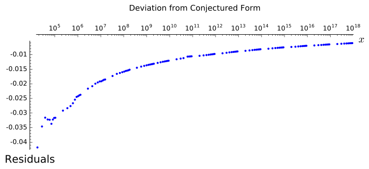
We compare (A.1) to the actual behavior of the primes, and find that because the approximations that were necessary to arrive at (A.1), the data deviate from the conjectured form. Using SageMath’s find_fit function suggested a possible lower order term of size O​((log2​x)2(log⁡x)2)O\quantity(\frac{(\log_2 x)^{2}}{(\log x)^2}). We modified the data gathering process to approximate values of π⁡(x,q,(a,b))\pi(x;q,(a,b)) for x≤1018x\leq 10^{18}. Finally, we include more terms in the approximation of 𝒟⁡(a,b,y)\mathcal{D}(a,b;y) to improve its accuracy in future work. Graphs may be found in Appendix B.

Lemke Oliver and Soundararajan [4] gathered values of π⁡(x,q,(a,b))\pi(x;q,(a,b)) up to x=1012x=10^{12}. We gathered data up to x=1018x=10^{18}. We gathered complete raw data using SageMath for 1≤x≤10101\leq x\leq 10^{10}. For 1010<x≤101810^{10}<x\leq 10^{18}, a sampling technique was used to approximate the ratio π⁡(x,q,(a,b))/π⁡(x)\pi(x;q,(a,b))/\pi(x). Lemke Oliver’s C++ code counts prime patterns in fixed intervals [X,Y)[X,Y); the program was modified to only consider the first 10810^{8} primes larger than XX. We used X=10b1X=10^{b_{1}} and Y=10b1+1Y=10^{b_{1}+1} for 10≤b1≤1810\leq b_{1}\leq 18. The program estimated pattern frequencies at X+i⋅10b1X+i\cdot 10^{b_{1}} for 1≤i≤91\leq i\leq 9.

Theorem 3.1 shows that the contributions S∅S_{\varnothing}, S{0}S_{\{0\}}, S{h}S_{\{h\}}, and S{0,h}S_{\{0,h\}} to 𝒟⁡(a,b,y)\mathcal{D}(a,b;y) decline quickly with nn. After dividing by li⁡(x)\mathrm{li}(x), the main terms in the main conjecture in [4] are of size O⁡(1)O(1), O⁡(log⁡log⁡xlog⁡x)O(\frac{\log\log x}{\log x}), and O⁡(1log⁡x)O(\frac{1}{\log x}). When |𝒯|=6\absolutevalue{\tset}=6, Theorem 3.1 implies that S∅∈O​((log2​y)6(log⁡y)2)S_{\varnothing}\in O\quantity(\frac{(\log_2 y)^6}{(\log y)^2}). Thus, for n≥6n\geq 6, S∅S_{\varnothing}, S{0}S_{\{0\}}, S{h}S_{\{h\}}, and S{0,h}S_{\{0,h\}} make negligible contributions to 𝒟\mathcal{D}. This implies that long range correlations between prime patterns are negligible, which in turn implies that even though we only take the first 10810^{8} primes after XX, the sample can be reasonably assumed to be unbiased.

Following Cramér’s model, we model primality as a binomial event with xx being prime with probability 1log⁡x\frac{1}{\log x} and assume that primality of xx and yy are independent events. Then the standard deviation of our sampling distribution is proportional to 1C\frac{1}{\sqrt{C}}, where CC is the number of primes sampled in order to estimate the frequency of π⁡(x,q,(a,b))\pi(x;q,(a,b)) at xx.

For each point estimate at X+i⋅10b1X+i\cdot 10^{b_{1}}, we sampled with C=108C=10^{8}, giving a precision of roughly 10−410^{-4}. The sample gives a sampling frequency

fa,b=π⁡(x+x0,q,(a,b))−π⁡(x,q,(a,b))π⁡(x+x0)−π⁡(x),f_{a,b}=\frac{\pi(x+x_{0};q,(a,b))-\pi(x;q,(a,b))}{\pi(x+x_{0})-\pi(x)},

where π⁡(x+x0)−π⁡(x)=107\pi(x+x_{0})-\pi(x)=10^{7}. In a crude sense, the sampling frequency fa,bf_{a,b} is the derivative of π⁡(x,q,(a,b))\pi(x;q,(a,b)), so we used a Riemann sum with 1010 equally spaced subintervals to estimate π⁡(X+i⋅10b1,q,(a,b))\pi(X+i\cdot 10^{b_{1}};q,(a,b)) from fa,bf_{a,b}. We thus computed

∑β=1b1∑α=19fa,b​[li⁡((α+1)⋅10β)−li⁡(α⋅10β)]li⁡(9⋅10b1).\frac{\sum_{\beta=1}^{b_{1}}\sum_{\alpha=1}^{9}f_{a,b}[\mathrm{li}((\alpha+1)\cdot 10^{\beta})-\mathrm{li}(\alpha\cdot 10^{\beta})]}{\mathrm{li}(9\cdot 10^{b_{1}})}. (A.2)

Note that (A.2) approximates the the ratio π⁡(10b1+1,q,(a,b))π⁡(x)\frac{\pi(10^{b_{1}+1};q,(a,b))}{\pi(x)} and hence allows us to extend our data to x=1018x=10^{18}.

We restate the conjectured form for π⁡(x,q,(a,b))\pi(x;q,(a,b)) as in Conjecture 2.2 for convenience as

π⁡(x,q,(a,b))∼1q​∫2xα​(y)ϵq​(a,b)​(qφ⁡(q)​α​(y)​log⁡y)2​𝒟​(a,b,y)​𝑑y.\pi(x;q,(a,b))\sim\frac{1}{q}\int_{2}^{x}\alpha(y)^{\epsilon_{q}(a,b)}\quantity(\frac{q}{\varphi(q)\alpha(y)\log y})^{2}\mathcal{D}(a,b;y)dy. (A.3)

The numerical model in [4] is evaluated by partitioning 𝒟⁡(a,b,y)\mathcal{D}(a,b;y) into ∑n𝒟n​(a,b,y)\sum_{n}\mathcal{D}_{n}(a,b;y) and discarding 𝒟n​(a,b,y)\mathcal{D}_{n}(a,b;y) for n≥3n\geq 3. Thus 𝔖q,0\mathfrak{S}_{q,0} is estimated only for zero and two term sets to approximate 𝒟⁡(a,b,y)\mathcal{D}(a,b;y). For example, in [4], only the zero and two term sets for 𝒟1​(a,b,y)\mathcal{D}_{1}(a,b;y) are considered. Lemke Oliver and Soundararajan then write

𝒟1(a,b;y)≈−qφ⁡(q)​α​(y)​log⁡y∑h>0h≡b−a(modq)∑t∈[1,h−1](t+a,q)=1𝔖q,0({0,t})+𝔖q,0({t,h}).\mathcal{D}_{1}(a,b;y)\approx-\frac{q}{\varphi(q)\alpha(y)\log y}\sum_{\begin{subarray}{c}h>0\\ h\equiv b-a\pmod{q}\end{subarray}}\sum_{\begin{subarray}{c}t\in[1,h-1]\\ (t+a,q)=1\end{subarray}}\mathfrak{S}_{q,0}(\{0,t\})+\mathfrak{S}_{q,0}(\{t,h\}). (A.4)

However, Theorem 3.1 suggests that only considering zero and two term sets may not accurate enough. Hence, we add terms to 𝒟0\mathcal{D}_{0}, 𝒟1\mathcal{D}_{1}, and 𝒟2\mathcal{D}_{2}, as well as truncating at 𝒟5\mathcal{D}_{5} instead of 𝒟2\mathcal{D}_{2} to approximate 𝒟\mathcal{D} in (A.3). For example, recalling that 𝒟1​(a,b,y)\mathcal{D}_{1}(a,b;y) contains all terms of (3.1) with |𝒯|=1\absolutevalue{\tset}=1, we write

𝒟1(a,b;y)=−qφ⁡(q)​α​(y)​log⁡y∑h>0h≡b−a(modq)∑t∈[1,h−1](t+a,q)=1𝔖q,0({0,t})+𝔖q,0({t,h})+𝔖q,0({0,t,h}).\mathcal{D}_{1}(a,b;y)=-\frac{q}{\varphi(q)\alpha(y)\log y}\sum_{\begin{subarray}{c}h>0\\ h\equiv b-a\pmod{q}\end{subarray}}\sum_{\begin{subarray}{c}t\in[1,h-1]\\ (t+a,q)=1\end{subarray}}\mathfrak{S}_{q,0}(\{0,t\})+\mathfrak{S}_{q,0}(\{t,h\})+\mathfrak{S}_{q,0}(\{0,t,h\}).

This is essentially (A.4) but with three term sets included. The values of singular series 𝔖q,0​(ℋ)\mathfrak{S}_{q,0}(\mathcal{H}) were computed up to five term sets with max⁡ℋ≤150\max\mathcal{H}\leq 150 and prepared for future work numerically integrating (A.3) by truncating at 𝒟5​(a,b,y)\mathcal{D}_{5}(a,b;y).

Appendix B Plots of Data and Model

This appendix contains the plots of raw data, extended data, curve fitting.

Refer to caption
Figure 1: The proportion π⁡(x,3,(1,1))π⁡(x)\frac{\pi(x;3,(1,1))}{\pi(x)} for x0≤x≤x1x_{0}\leq x\leq x_{1} where π⁡(x0)=104\pi(x_{0})=10^{4} and π⁡(x1)=109\pi(x_{1})=10^{9}.
Refer to caption
Figure 2: The extended data for (1,1)(1,1) modulo 33. The slight bump at 5⋅10105\cdot 10^{10} is due to combining the raw and sampled data.
Refer to caption
Figure 3: The extended data for (1,2)(1,2) modulo 33. The slight bump at 5⋅10105\cdot 10^{10} is due to stitching the raw data and sampled data together.
Refer to caption
Figure 4: The residuals when (A.1) is subtracted from π⁡(x,3,(1,1))\pi(x;3,(1,1)) for x0≤x≤x1x_{0}\leq x\leq x_{1} where π⁡(x0)=104\pi(x_{0})=10^{4} and π⁡(x1)=1018\pi(x_{1})=10^{18}, using the extended data.
Refer to caption
Figure 5: The residuals when curve fitted terms of size O⁡((log2​y)2/(log⁡y)2)O((\log_{2}y)^{2}/(\log y)^{2}) and (A.1) are subtracted from π⁡(x,3,(1,1))\pi(x;3,(1,1)) for x0≤x≤x1x_{0}\leq x\leq x_{1} where π⁡(x0)=104\pi(x_{0})=10^{4} and π⁡(x1)=1018\pi(x_{1})=10^{18}, using the extended data.

References

  • [1] T. M. Apostol, Introduction to Analytic Number Theory. Springer, 1998.
  • [2] P. G. L. Dirichlet, Beweis des Satzes, dass jede unbegrenzte arithmetische Progression, deren erstes Glied und Differenz ganze Zahlen ohne gemeinschaftlichen Factor sind, unendlich viele Primzahlen enthält, p. 342–359. Cambridge Library Collection - Mathematics, Cambridge University Press, 2013.
  • [3] L. Schoenfeld, “Sharper Bounds for the Chebyshev functions θ⁡(x)\theta(x) and ψ⁡(x)\psi(x). ii,” Mathematics of Computation, vol. 30, no. 134, pp. 337–360, 1976.
  • [4] R. J. L. Oliver and K. Soundararajan, “Unexpected biases in the distribution of consecutive primes,” 2016.
  • [5] “Lettre de M. le Professeur Tchébychev à M. Fuss sur un nouveaux théorème relatif aux nombres premiers contenus dans les formes 4​n+14n+1 et 4​n+34n+3,” 1853.
  • [6] M. Rubinstein and P. Sarnak, “Chebyshev’s bias,” Experiment. Math., vol. 3, no. 3, pp. 173–197, 1994.
  • [7] D. K. Shiu, “Strings of congruent primes,” Journal of the London Mathematical Society, vol. 61, no. 2, pp. 359–373, 2000.
  • [8] J. Maynard, “Dense clusters of primes in subsets,” Compositio Mathematica, vol. 152, no. 7, pp. 1517–1554, 2016.
  • [9] H. L. Montgomery and K. Soundararajan, “Primes in short intervals,” Communications in Mathematical Physics, 2004.
  • [10] P. Gallagher, “On the distribution of primes in short intervals,” Mathematika, vol. 23, no. 1, pp. 4–9, 1976.