New Loop Quantum Cosmology Modifications from Gauge-covariant Fluxes

We begin by outlining the classical continuum phase space $(M,\Omega)$ of GR in the Ashtekar-Barbero variables on a spatial manifold $\sigma$. Here $M$ denotes the pair of canonical phase variables: connections $A^{I}_{a}(x)\tau_{I}$ and electric fields $E^{b}_{J}(y)\tau_{J}$ respectively, and $\Omega$ is a symplectic structure. $\tau_{I}=i\sigma_{I}/2$ ($I=1,2,3$) denote the generators of the Lie algebra $\mathfrak{su}(2)$, satisfying $\mathrm{tr}(\tau_{I}\tau_{J})=-\delta_{IJ}/2$ with $\sigma_{I}$ as the Pauli matrices. Using

$$\Omega=\frac{2}{\kappa\gamma}\int_{\sigma}{\rm d}^{3}x\;{\rm d}E^{a}_{I}(x)\wedge{\rm d}A^{I}_{a}(x)$$

(1)

we can define the Poisson bracket through $\{f,g\}:=\Omega(\chi_{f},\chi_{g})$. Explicitly, for a vector density test field $F^{a}_{I}$ of weight one and a covector test field $f^{I}_{a}$, one obtains for the smeared quantities

$\displaystyle A[F]:=\int_{\sigma}{\rm d}^{3}x\;F^{a}_{I}A^{I}_{a}\hskip 30.0pt{\rm and}\hskip 30.0ptE[f]:=\int_{\sigma}{\rm d}^{3}x\;E^{a}_{I}f^{I}_{a}~,$

(2)

the following Poisson brackets

$\displaystyle\{E[f],E[f^{\prime}]\}=0=\{A[F],A[F^{\prime}]\},\hskip 30.0pt\{E[f],A[F]\}=\frac{\kappa\gamma}{2}\int_{\sigma}{\rm d}^{3}x\;F^{a}_{I}f^{I}_{a}$

(3)

where $\kappa=16\pi G$ is the gravitational coupling constant and $\gamma\in\mathbb{R}$ is the Barbero-Immirzi parameter.

We will now consider a truncation of $(M,\Omega)$ to a given graph $\Gamma$. The graph $\Gamma$ we consider is a cubic lattice (with possibly infinitely many vertices SahThiWin). This graph shall be adapted to a fiducial metric $\eta$ in such a way that the edges of its three directions are along the 3-axes of coordinates. The coordinate length of each edge is $\epsilon>0$ with respect to $\eta$.

Constructed in this way, $\Gamma$ allows the definition of a dual cell-complex of faces which is unique up to diffeomorphisms. We choose its precise form with respect to the fiducial metric $\eta$ in the following way ThiemanComplex. To each edge $e$ of $\Gamma$ we assign an open face $S_{e}$ carrying the same orientation as $e$ and such that (i) the faces are mutually non-intersecting, (ii) only $e$ intersects $S_{e}$, (iii) the intersection happens only in one point $e(1/2)$ whose distance to start and end of the edge is both measured as $\epsilon/2$ with respect to $\eta$, and, (iv) if $e$ is oriented along direction $k$ then $S_{e}$ is oriented along the directions orthogonal to $k$.

Along the lines of ThiVII00 we define the discrete symplectic manifold $(M_{\Gamma},\Omega_{\Gamma})$ coming from the continuum $(M,\Omega)$:

The first advantage of using functions $h(e),P(e)$ is that their behavior under gauge transformation is well understood. The ${\rm SU}(2)$-Gauss constraint (whose vanishing must be imposed to the restrict the phase space of the Ashtekar-Barbero variables to one equivalent with GR) implies the following Hamiltonian flow on the phase space variables

$\displaystyle A_{a}(x)\mapsto-(\partial_{a}g)(x)g^{-1}(x)+g(x)A_{a}(x)g^{-1}(x)\hskip 20.0pt{\rm and}\hskip 20.0ptE^{a}(x)\mapsto g(x)E^{a}(x)g^{-1}(x)$

(6)

for any field $g:\sigma\to{\rm SU}(2)$. Using above we find that a holonomy $h(e)$ of the path $e$ transforms as

$\displaystyle h(e)\mapsto g(e(0))h(e)g^{-1}(e(1))~,$

(7)

where $e(0)$ is the beginning point and $e(1)$ is the final point of the path $e$. In contrast to the standard fluxes, the gauge-covariant flux $P(e)$ transforms covariantly

$\displaystyle P^{J}(e)\tau_{J}\mapsto g(e(0))P^{J}(e)\tau_{J}g^{-1}(e(1))~.$

(8)

This fact allows the construction of discretized phase space functions, which are gauge-invariant even before removal of the regulator. As a concrete example, consider a family of lattices $\{\Gamma_{\epsilon}\}_{\epsilon}$ such that they lie infinitely dense in $\sigma$ for $\epsilon\to 0$. Let $v\in\sigma$ be a vertex of $\Gamma_{\epsilon}$ $\forall\epsilon$ then

$\displaystyle Q^{\epsilon}(v):=\frac{1}{3!}\sum_{e_{1}\cap e_{2}\cap e_{3}=v}\epsilon(e_{1},e_{2},e_{3})\epsilon_{IJK}P^{I}(e_{1})P^{J}(e_{2})P^{K}(e_{3})\underset{\epsilon\to 0}{\longrightarrow}\det(E)(v)=Q(v)~.$

(9)

In other words $Q^{\epsilon}(v)$ is a discretization of the continuum function $Q(v)$ while being gauge-invariant for all $\epsilon$.¹¹ 1 Note that the necessity of implementing a flux that transforms covariantly disappears if one considers everything the limit of infinitesimal faces. Given that the fluxes reduce to the triad itself for vanishing regulator, its gauge-transformation is restored in the continuum limit. Of course, this is exactly what has been done in standard LQG in order to build geometrical operators RS94; AL96; AL98; Thi98a; Thi98b.

The second advantage of using the functions $P(e)$ in contrast to the standard smeared fluxes, is that it was proven in ThiVII00 how a natural Poisson bracket arises for each $(M_{\Gamma},\Omega_{\Gamma})$.²² 2 This was done in the presence of regulated tubes around the holonomies and thick surfaces. The brackets are then computed in presence of the regulator, which can afterwards be removed smoothly. We refer the reader to ThiVII00 for various details. In particular, we are interested in the following theorem ThiVII00:

With the algebra (10)-(12) at hand, canonical quantization on the fixed lattice can now be carried out as is standard in the literature KS75. Indeed, following the usual procedure in LQG and promoting holonomies to multiplication operators and gauge-covariant fluxes to right-invariant vector fields ($f\in\mathcal{H}_{\Gamma}$):

	$\displaystyle\hat{h}_{mn}^{(1/2)}(e^{\prime})f(\{g_{e}\}_{e\in\Gamma}):=D^{(1/2)}_{mn}(g_{e^{\prime}})f(\{g_{e}\}_{e\in\Gamma})$		(13)
	$\displaystyle\hat{P}^{I}(e^{\prime})f(\{g_{e}\}_{e\in\Gamma}):=\frac{-i\hbar\kappa\gamma}{2}R^{K}(e^{\prime})f(\{g_{e}\}_{e\in\Gamma}),$		(14)

one finds that these satisfy commutation relations which exactly agree with the canonical quantization rule $i\hbar\{.,.\}\to[.,.]$. Namely,

	$$\displaystyle[\hat{h}^{(1/2)}(e),\hat{h}^{(1/2)}(e^{\prime})]=0,\hskip 30.0pt[R^{K}(e),\hat{h}^{(1/2)}(e^{\prime})]=\delta_{ee^{\prime}}\tau_{K}\;\hat{h}^{(1/2)}(e^{\prime})$$		(15)
	$$\displaystyle[R^{I}(e),R^{J}(e^{\prime})]=-\delta_{ee^{\prime}}\epsilon_{IJK}R^{K}(e)~.$$		(16)

In this framework based on a finite lattice it is hence easy to understand the functions $P^{I}(e)$ as the semiclassical limit of the operators (14), since the commutator algebra reflects the classical Poisson bracket algebra. A coherent state in $\mathcal{H}_{\Gamma}$ should therefore be chosen such that it is peaked on $P^{I}(e)$ instead of the standard smeared fluxes $E^{I}(S)$. This is exactly what has been proposed in Winkler1; Winkler2; Winkler3; ThiemanComplex; SahThiWin.

In the following, we will hence adopt this strategy and regularize all physical quantities as functions of $h(e),P^{I}(e)$, as, e.g., shown in (9) for the square of the volume of a single cell. More complicated operators like the scalar constraint can be regularized following a similar strategy LL19.

Following the coherent state method of computing expectation values, we will in the this section compute $P^{I}(e)$ explicitly of a cubic lattice $\Gamma$ with spacing $\epsilon>0$ for isotropic, spatially-flat FLRW cosmology.

In a certain gauge-fixing the Ashtekar-Barbero variables for an isotropic spatially-flat metric can be expressed as,

$\displaystyle A^{I}_{a}(x)=c\;\delta^{I}_{a},\hskip 40.0ptE^{a}_{I}(x)=p\;\delta^{a}_{I}$

(17)

where $|p|=V_{o}^{2/3}a^{2}$ and $c=\gamma V_{o}^{1/3}\dot{a}/\tilde{N}$ (only for the classical GR). Here $\tilde{N}$ is the lapse and $V_{0}:=\int_{\sigma_{M}}d^{3}x$ is the coordinate volume of a compact subset $\sigma_{M}\subset\sigma$, which we will choose to be a torus $T^{3}$ with $V_{0}=1$ in the following. We can think of $(c,p)$ as coordinatizing the subspace of the GR phase space representing spatially-flat, isotropic cosmology with a reduced symplectic structure:

$\displaystyle\Omega_{\rm cos}=\frac{6}{\kappa\gamma}{\rm d}p\wedge{\rm d}c$

(18)

from which the Poisson bracket on the reduced space follows:³³ 3 The reader should note, that there exists two conventions in LQG literature for the Poisson-bracket. The one commonly used in LQC reads $\{p,c\}=-\kappa\gamma/6$. The additional minus sign, however, has no consequences for physical quantities, so we will stick to (19) in the following.

$$\{p,c\}=\frac{\kappa\gamma}{6}~.$$

(19)

Computing the standard fluxes for the face in the dual cell-complex to a lattice $\Gamma$ oriented along the coordinate axes with coordinate spacing $\epsilon$ one finds,

$$h(e_{k})=\exp(\int_{0}^{1}{\rm d}t\;c\delta^{J}_{a}\tau_{J}(\epsilon\delta_{k}^{a}))=e^{c\epsilon\tau_{k}}=\cos(\frac{c\epsilon}{2})\mathds{1}+2\sin(\frac{c\epsilon}{2})\tau_{k}$$

(20)

for an holonomy oriented along direction $k$ and

$$E^{I}(e_{k})=\int_{S_{e_{k}}}(\ast E_{I})(x)=\int_{-\epsilon/2}^{\epsilon/2}{\rm d}u\int_{-\epsilon/2}^{\epsilon/2}{\rm d}v\;p\delta^{I}_{k}=\epsilon^{2}p\delta^{I}_{k}.$$

(21)

In order to compare this with the gauge-covariant fluxes $P(e)$, one has to choose a certain set of paths $\rho$ in their construction (5). For the moment, we choose for an edge $e_{k}$ oriented along coordinate direction $k$ to split $\rho_{x}=\rho_{x,a}\circ\rho^{\prime}_{x,b}$ where $\epsilon_{kab}=1$. The path $\rho_{x,a}$ starts from the intersection point $\rho_{x,a}[0]=e_{k}\cap S_{e_{k}}$ in direction $\pm a$, stays in $S_{e_{k}}$ and its tangent vector remains constant. The end point of this path, i.e. $\rho_{x,a}[1]$, agrees with the starting point of $\rho^{\prime}_{x,b}$ and is chosen such that the latter path has a constant tangent vector oriented along $\pm b$ and ends in point $x$, i.e. $\rho^{\prime}_{x,b}[1]=x$.

Let $k>0$ and $\epsilon_{kab}=1$. Then

	$\displaystyle P^{I}(e_{k})=$	$\displaystyle-2\,\mathrm{tr}\bigg(\tau_{I}[\cos(\frac{c\epsilon}{4})\mathds{1}+2\sin(\frac{c\epsilon}{4})\tau_{k}]\int_{-\epsilon/2}^{\epsilon/2}{\rm d}u_{a}\int_{-\epsilon/2}^{\epsilon/2}{\rm d}u_{b}\;h(\rho_{x(u_{a},u_{b}),a})\times$		(22)
		$\displaystyle\hskip 5.0pt\times h(\rho^{\prime}_{x(u_{a},u_{b}),b})\epsilon_{abd}E^{d}(x(u_{a},u_{b}))h(\rho^{\prime}_{x(u_{a},u_{b}),b})^{-1}h(\rho^{\prime}_{x(u_{a},u_{b}),a})^{-1}[\cos(\frac{c\epsilon}{4})\mathds{1}+2\sin(\frac{c\epsilon}{4})\tau_{k}]\bigg)$

where we choose a coordinate system of $S_{e_{k}}$ to parametrize the points $x=x(u_{a},u_{b})$. Note that

	$\displaystyle\int_{-\epsilon/2}^{\epsilon/2}{\rm d}u_{b}\;h(\rho^{\prime}_{x(u_{a},u_{b}),b})\epsilon_{abd}E^{d}(x(u_{a},u_{b}))h(\rho^{\prime}_{x(u_{a},u_{b}),b})^{-1}$				(23)
			$\displaystyle\hskip-227.62204pt=\int_{-\epsilon/2}^{\epsilon/2}{\rm d}u_{b}[\cos(\frac{cu_{b}}{2})\mathds{1}+2\sin(\frac{cu_{b}}{2})\tau_{J}]p\tau_{K}\delta^{K}_{k}[\cos(\frac{cu_{b}}{2})\mathds{1}-2\sin(\frac{cu_{b}}{2})\tau_{J}]$
			$\displaystyle\hskip-227.62204pt=\int_{-\epsilon/2}^{\epsilon/2}{\rm d}u_{b}\;p\;\delta^{K}_{k}[\cos^{2}(\frac{cu_{b}}{2})\tau_{K}-4\sin^{2}(\frac{cu_{b}}{2})\tau_{J}\tau_{K}\tau_{J}]=\int_{-\epsilon/2}^{\epsilon/2}{\rm d}u_{b}\;p\;\delta^{K}_{k}[\cos(cu_{b})]\tau_{K}$
			$\displaystyle\hskip-227.62204pt=p\;\delta^{K}_{k}\tau_{K}\frac{\sin(c\epsilon/2)}{c/2}$

where we used the vanishing of odd functions under the integral, $\tau_{J}\tau_{K}\tau_{J}=\tau_{K}/4$ if $J\neq K$, and $\cos^{2}(x)-\sin^{2}(x)=\cos(2x)$. As the result of (23) is again proportional to $\tau_{k}$, the same calculation goes through for the integral over $u_{a}$. Finally, using $\tau_{I}^{2}=-1/4$, $-2\mathrm{tr}(\tau_{I}\tau_{J})=\delta_{IJ}$ and $\mathrm{tr}(\tau_{I})=0$ we obtain

	$\displaystyle P^{I}(e_{k})$	$\displaystyle=-2\,\mathrm{tr}\left(\tau_{I}[\cos(\frac{c\epsilon}{4})\mathds{1}+2\sin(\frac{c\epsilon}{4})\tau_{k}]\tau_{k}[\cos(\frac{c\epsilon}{4})\mathds{1}-2\sin(\frac{c\epsilon}{4})\tau_{k}]\right)p\frac{\sin^{2}(c\epsilon/2)}{(c/2)^{2}}$
		$\displaystyle=[\delta^{I}_{k}\cos(\frac{c\epsilon}{4})^{2}+\delta^{I}_{k}\frac{1}{4}4\sin^{2}(\frac{c\epsilon}{4})]p\frac{\sin^{2}(c\epsilon/2)}{(c/2)^{2}}=(\epsilon^{2}p\;\delta^{I}_{k})\;\frac{\sin^{2}(c\epsilon/2)}{(c\epsilon/2)^{2}}$
		$\displaystyle=E^{I}(e_{k})\;{\rm sinc}^{2}(c\epsilon/2)~.$		(24)

The remarkable property of this result is, that it allows us to pass from the known expressions in the literature using the standard fluxes directly to the gauge-covariant fluxes by simply replacing $p\to p\;{\rm sinc}^{2}(c\epsilon/2)$. One can hence avoid repetition of lengthy computation of expectation-values of coherent states, and instead immediately obtain results by using the gauge-covariant flux in expressions of DL17a; DL17b; LL19. In other words, the leading contribution will be nothing else but the regularization of the scalar constraint in the presence of the gauge-covariant fluxes.

Motivated by these findings, we will close this section by giving an explicit example, of how such a gauge-invariant regularization looks like. For the purpose of this example, we choose the scalar constraint where the Lorentzian part is put proportional to the so-called Euclidean part.⁴⁴ 4 One might take the point of view, that we restrict partially to cosmology before discretization. Such a restriction leads to this symmetry, as the curvature term of the scalar constraint vanishes. Moreover, we add a homogeneous, massless, free scalar field $\phi$ minimally coupled to gravity, which can play the role of a relational clock. The Hamiltonian constraint in this case is given by,

$\displaystyle C[\tilde{N}]=\int{\rm d}^{3}x\;\tilde{N}\left(\frac{1}{\kappa\gamma^{2}}\frac{\epsilon^{IJK}E^{a}_{J}E^{b}_{K}}{\sqrt{|\det(E)|}}F^{I}_{ab}+\frac{\pi_{\phi}^{2}}{2\sqrt{|\det(E)|}}\right)$

(25)

where $\pi_{\phi}$ is the canonical conjugated momentum to $\phi$.

We use the standard regularization strategy from Thi98a; Thi98b, where the curvature of the connection gets approximated by a loop $\Box^{\epsilon}$ and the volume of a small region by $\sqrt{|Q^{\epsilon}|}$ from (9). Using the homogeneity symmetry of the cosmological model, this leads finally to the regularized expression:

	$\displaystyle C^{\epsilon}[\tilde{N}]$	$\displaystyle=$	$\displaystyle\frac{-4\tilde{N}}{48\kappa^{2}\gamma^{3}}\sum_{ijk}\epsilon(i,j,k)\mathrm{tr}\left((h(\Box^{\epsilon}_{ij})-h(\Box^{\epsilon}_{ji})h(e_{k})\{h(e_{k}^{-1},\sqrt{|Q^{\epsilon}|}\}\right)+\frac{\tilde{N}\pi_{\phi}^{2}}{2\sqrt{|Q^{\epsilon}|}}$		(26)
		$\displaystyle=$	$\displaystyle-\frac{6\tilde{N}}{\kappa\gamma^{2}}\frac{\sin^{2}(c\epsilon)}{\epsilon^{2}}\sqrt{|p|}\;{\rm sinc}(c\epsilon/2)+\frac{\tilde{N}\pi_{\phi}^{2}}{2\sqrt{|p^{3}|}}{\rm sinc}^{-3}(c\epsilon/2)~.$

Like any suitable regularization it holds that $\lim_{\epsilon\to 0}C^{\epsilon}[\tilde{N}]=C[\tilde{N}]$ and the deviation from earlier regularizations considered in the literature APS06a; APS06b; APS06c is in the aforementioned presence of the ${\rm sinc}$-terms. It is the impact of these non-trivial corrections which we will study in the further sections of this article.

We emphasize that this classical discretization can serve as the starting point of a loop quantization, where the holonomy-flux algebra gets promoted to operators along (15). In order to ensure normalizability, the associated Hilbert space is then chosen as the set of possibly all finite graphs. For example the subset of cubic graphs with periodic boundary condition can represent a suitable discretization of the compact torus $\sigma_{M}\subset\sigma$.

This choice of the regulator appeared in the earliest works in LQC, and is based on considering the minimum square area of the loops over which holonomies are constructed, with respect to the fiducial metric, and equating it with the minimum non-zero eigenvalue $\Delta=4\sqrt{3}\pi\gamma\ell^{2}_{P}$ of the area operator in LQG abl; Boj05; APS06a; APS06b which results in:

$$\epsilon=\mu_{0},\hskip 30.0pt\mu_{0}:=3\sqrt{3}~$$

(27)

In the following, we will choose natural units $\ell_{P}=G=\hbar=c=1$.

The vanishing of the Hamiltonian constraint (26) immediately results in the following expression of energy density:

$$\rho=\frac{6}{\kappa\gamma^{2}\mu_{0}^{2}}p^{1/2}\sin^{2}(c\mu_{0}){\rm sinc}^{-2}(c\mu_{0}/2)~.$$

(28)

From this expression we see that there is no global bound for the energy density in the dynamical evolution in the $\mu_{0}$ scheme (as is the situation in standard LQC). Depending on the value of the triad $p$ at which the quantum bounce occurs, which in turn is determined by the value of $\pi_{\phi}$, the energy density at the bounce changes and can be much smaller or larger than the Planckian value.

The Hamilton’s equation can be computed using (26) which turn out to be (when choosing lapse $\tilde{N}=1$)

	$\displaystyle\dot{c}$	$\displaystyle=$	$\displaystyle-\frac{1}{2\sqrt{p}\gamma}\frac{\sin^{2}(c\mu_{0})}{\mu_{0}^{2}}{\rm sinc}(c\mu_{0}/2)-\frac{\pi_{\phi}^{2}\gamma\kappa}{8p^{5/2}}{\rm sinc}^{-3}(c\mu_{0}/2)~,$		(29)
	$\displaystyle\dot{p}$	$\displaystyle=$	$\displaystyle\frac{1}{16\mu_{0}\gamma p^{3/2}{\rm sinc}^{2}\left(\frac{c\mu_{0}}{2}\right)}\Bigg[8p^{2}\cos\left(\frac{c\mu_{0}}{2}\right)\text{sinc}^{4}\left(\frac{c\mu_{0}}{2}\right){}\left(c\mu_{0}-2\sin\left(c\mu_{0}\right)+5c\mu_{0}\cos\left(c\mu_{0}\right)\right)$		(30)
			$\displaystyle~~~~~+\gamma^{2}\kappa\mu_{0}^{2}\pi_{\phi}^{2}\left(c\mu_{0}\cot\left(\frac{c\mu_{0}}{2}\right)-2\right)\csc\left(\frac{c\mu_{0}}{2}\right)\Bigg]~,$
	$\displaystyle\dot{\phi}$	$\displaystyle=$	$\displaystyle\frac{\pi_{\phi}}{p^{3/2}}{\rm sinc}^{-3}(c\mu_{0}/2)~,$		(31)
	$\displaystyle\dot{\pi}_{\phi}$	$\displaystyle=$	$\displaystyle 0~.$		(32)

These equations can be numerically solved, a representative of which are plotted in Fig. 1. From these plots we see a bounce of the volume of the universe along with boundedness of $\mu_{0}c$, $\rho$ and Hubble rate $H$. Before we discuss these plots, and differences from standard LQC, it is instructive to study the asymptotic behavior of $C^{\mu_{0}}[\tilde{N}]$ in post-bounce and pre-bounce phases. In particular, we wish to understand the form of the (modified) Friedmann equation and Raychaudhuri equation far away from the bounce, at very large volumes or equivalently very small energy density.

As in standard LQC, it is clear from $C^{\mu_{0}}[\tilde{N}]=0$ that $\rho$ will become small around the zeros of $\sin(c\mu_{0})$. Choosing some of those, we expand around $c=0,\pi/\mu_{0}$.⁶⁶ 6 As the numerical investigation below demonstrates, it suffices to study the expansion around these two points. Given suitable initial conditions, the dynamics drives exactly to these asymptotes. If one chooses one of these points to correspond to post-bounce regime, the other corresponds to the pre-bounce regime (see Fig. 1). Around $c\simeq 0$ the scalar constraint from (26) becomes (neglecting all contributions higher than $c^{3}$)

$\displaystyle C^{\mu_{0}}[\tilde{N}]\overset{c\simeq 0}{=}\frac{6\tilde{N}}{\kappa\gamma^{2}}\sqrt{p}c^{2}+\frac{\tilde{N}\pi_{\phi}^{2}}{2p^{3/2}}(1+\frac{c^{2}\mu_{0}^{2}}{8})+\mathcal{O}(c^{4})\approx 0~.$

(33)

This can be solved for $c$ as:

$$c=\pm\frac{\pi_{\phi}\sqrt{\kappa\gamma^{2}}}{p\sqrt{12}}\sqrt{1-\frac{\mu_{0}^{2}\pi_{\phi}^{2}\kappa\gamma^{2}}{96p^{2}}}^{-1}~.$$

(34)

We can then obtain the following Hamilton’s equation in the limit of large $p$:

$\displaystyle\dot{p}=\{C^{\mu_{0}}[\tilde{N}],p\}=\tilde{N}\frac{\sqrt{p}}{\gamma}\frac{\sin(2c\mu_{0})}{\epsilon}{\rm sinc}(c\mu_{0}/2)+\mathcal{O}(p^{-3/2})~.$

(35)

We eliminate therein $c$ using (34) to obtain the Friedmann equation. Similarly we can use $\ddot{a}=\{C[\tilde{N}],\dot{p}/(2\sqrt{p})\}$ to determine the Raychaudhuri equation. Together they read:

	$\displaystyle\left(\frac{\dot{a}}{a}\right)^{2}|_{c\simeq 0}$	$\displaystyle=\tilde{N}^{2}\frac{\kappa}{6}\frac{\pi_{\phi}^{2}}{2p^{3}}+\mathcal{O}(p^{-4})~,$		(36)
	$\displaystyle\left(\frac{\ddot{a}}{a}\right)|_{c\simeq 0}$	$\displaystyle=-\tilde{N}^{2}\frac{\kappa}{3}\frac{\pi_{\phi}^{2}}{2p^{3}}+\mathcal{O}(p^{-4})~.$		(37)

As it turns out this agrees in its leading order in the matter energy density with the classical Friedmann and Raychaudhuri equations, which are commonly written with $\tilde{N}=1$. Note that in the above equations, since ${\rm sinc}(c\mu_{0})|_{c\simeq 0}\simeq 1$ one gets $p_{\rm{g.c.}}\simeq p$. As a result, the energy density $\rho={\cal H_{M}}/p^{3/2}_{\rm{g.c.}}$ for the massless scalar field equals the conventional expression $\pi_{\phi}^{2}/2p^{3}$. Hence, we find that in the presence of gauge-covariant flux modifications the asymptotic regime in the neighborhood of $c\simeq 0$ agrees with the one of classical GR.

As already mentioned, another obvious phase space point for small $\rho$ is at $c=\pi/\mu_{0}$. To determine the effective Friedmann equation at this point, we perform a canonical transformation $c^{*}:=\pi/\mu_{0}-c$ and proceed again as before:

$\displaystyle C^{\mu_{0}}[\tilde{N}]\overset{c^{*}\simeq 0}{=}-\frac{6\tilde{N}}{\kappa\gamma^{2}}{c^{*}}^{2}\sqrt{p}\frac{1-(c^{*}\mu_{0}/2)^{2}}{\pi/2-c^{*}\mu_{0}/2}+\frac{\tilde{N}\pi_{\phi}^{2}}{2p^{3/2}}\left(\frac{1-(c^{*}\mu_{0}/2)^{2}/2}{\pi/2-c^{*}\mu_{0}/2}\right)^{-3}+\mathcal{O}({c^{*}}^{3})\approx 0$

(38)

which can be solved for $c^{*}$ as:

$\displaystyle c^{*}=\pm\frac{\pi_{\phi}\sqrt{\kappa\gamma^{2}}}{p\sqrt{12}}\left(\frac{\pi}{2}\right)^{2}+\mathcal{O}(p^{-2})~.$

(39)

We see, that this is already at leading order different than (34), which is caused by the expansion of ${\rm sinc}$ around $\pi/2$.

Once again, this will be inserted into $\dot{p}$ as determined by the Hamiltonian flow of the constraint. In the same manner, we determine $\ddot{a}$ via the flow of the constraint and after some algebra we find modified Friedmann and Raychaudhuri equations:

	$\displaystyle\left(\frac{\dot{a}}{a}\right)^{2}|_{c\simeq\pi/\mu_{0}}$	$\displaystyle=$	$\displaystyle\tilde{N}^{2}\frac{\kappa}{6}\frac{\pi_{\phi}^{2}}{2p^{3}}{\rm sinc}^{-2}(\pi/2)+\mathcal{O}(p^{-4})=\tilde{N}^{2}\frac{\kappa}{6}\frac{\pi_{\phi}^{2}}{2p^{3}}\left[\frac{\pi}{2}\right]^{2}+\mathcal{O}(p^{-4}),$		(40)
	$\displaystyle\left(\frac{\ddot{a}}{a}\right)|_{c\simeq\pi/\mu_{0}}$	$\displaystyle=$	$\displaystyle-\tilde{N}^{2}\frac{\kappa}{3}\frac{\pi_{\phi}^{2}}{2p^{3}}{\rm sinc}^{-2}(\pi/2)+\mathcal{O}(p^{-4})=-\tilde{N}^{2}\frac{\kappa}{3}\frac{\pi_{\phi}^{2}}{2p^{3}}\left[\frac{\pi}{2}\right]^{2}+\mathcal{O}(p^{-4})~.$		(41)

These equations are manifestly different from the classical expression. Moreover, one realizes that unlike the case of $c=0$, the velocity of the scalar field is modified around $c=\pi/\mu_{0}$, namely

$\displaystyle\dot{\phi}|_{c\simeq\pi/\mu_{0}}=\{C^{\mu_{0}}[\tilde{N}],\phi\}|_{c\simeq\pi/\mu_{0}}=\tilde{N}\frac{\pi_{\phi}}{\sqrt{p}^{3}}\left[\frac{\pi}{2}\right]^{3}+\mathcal{O}(p^{-4})~.$

(42)

Above equations imply that one can find a rescaling of $\tilde{N}$, $\pi_{\phi}$ and $G$ as

$\displaystyle\bar{\pi}_{\phi}=\pi_{\phi}\alpha,\hskip 50.0pt\bar{N}=\tilde{N}\left[\pi/2\right]^{3}\alpha^{-1},\hskip 50.0pt\bar{G}=G\left[2/\pi\right]^{4}$

(43)

such that for any $\alpha\in\mathbb{R}$\$\{0\}$ the dynamical equations take again the form of classical Friedmann equations with rescaled scalar field momentum $\bar{\pi}_{\phi}$ and with modified Newton’s coupling constant $\bar{G}$ and new lapse $\bar{N}$. The freedom in choice of $\alpha$ implies that one could for example absorb the rescaling of lapse completely in $\pi_{\phi}$ . On the other hand, it also possible to choose $\alpha=1$, i.e. we merely rescale the lapse function, which reflects simply a choice of coordinate system and has therefore no physical relevance.⁷⁷ 7 This can be also seen, when realizing that relational observables, such as $v(\phi)$, do classically not depend on $\pi_{\phi}$, which is seen therefore to be pure gauge in the $v-\phi$ plane. Thus, if one chooses $\alpha=1$, one isolates the physically relevant rescaling of $G\to\bar{G}$.

Given the observational constraints on $G$, this asymptotic regime is ruled out to represent the post-bounce expanding branch of our universe, and can only correspond to the pre-bounce phase (see Ref. LSW18a for a discussion on a similar constraint). Thus, in the asymptotic pre-bounce regime, the dynamical equations from (26) correspond to classical Friedmann and Raychaudhuri equations expressed in standard scale factor (or triads) with a modified Newton’s coupling constant given by (43).

We want to point out, that there also exists a second branch of solutions, which are the time-reversed version of the former. If one expands the Friedmann equations around the point $c=-\pi/\mu_{0}$, one finds another classical asymptote with the same rescaling. However, this solution has to be interpreted in such a way that the rescaled universe lies in the post-bounce branch. Of course, the previous analysis can in principle be repeated for all $b:=c\bar{\mu}\simeq z\pi$ with $z\in\mathbb{Z}$. In standard LQC these choices corresponded to several branches, which were all physically indistinguishable as the flow of the Hamiltonian constraint in standard LQC interpolates between $(z-1)\pi$ and $z\pi$. In that case each point $z\pi$ corresponds to an asymptotic point where classical FLRW universe gets approached. As a result, in standard LQC it is not possible to decide the corresponding branch of the universal dynamics from physical observations.

However, in presence of the gauge-covariant fluxes the situation changes dramatically. Similar to (40), at $c\mu_{0}\simeq z\pi$ the rescaling in the Friedmann and Raychaudhuri equations goes as ${\rm sinc}(z\pi/2)^{-2}$. In other words, the only two branches featuring as classical FLRW universe in one asymptotic limit are the two principal branches $c\in(-\pi/\mu_{0},0)$ and $c\in(0,\pi/\mu_{0})$. It should be noted that one principal branch is exactly the time reverse version of the other principal branch. That means that if initial conditions are given in the pre-bounce branch, then a rescaling of constants occurs for the post-bounce branch. The asymptotic properties of the solutions, as discussed above, show that the rescaling $G\to\bar{G}\neq G$ is an intrinsic feature of the Hamiltonian with gauge-covariant flux modifications. This rescaling holds irrespective of the initial conditions. Thus, there is no choice for $G$ such that the effective Newton’s constant as measured on both sides of the bounce is the same. The same result holds true for the $\bar{\mu}$-scheme.

In summary, it transpires that the quantum evolution through the bounce will be asymmetric by connecting two phase space points of classical/rescaled FLRW. This is confirmed by the numerical solutions for which we consider Barbero-Immirzi parameter $\gamma=0.2375$, and choose as initial state at late times a universe with $p(t_{0})=6\times 10^{4}$, $\phi(t_{0})=13.5$ and $\pi_{\phi}(t_{0})=300$ with $t_{0}=0$. From the Hamilton’s equations we see that the latter value turns out to be a constant of motion. Further, the initial condition for $\phi$ plays little role because of the rescaling freedom in $\phi$ since the Hamiltonian constraint is $\phi$ independent. The corresponding initial value of $c(t_{0})$ can be determined by implementing the Hamiltonian constraint. Figs. 1 and 2 show the evolution of volume, Hubble rate, connection and energy density confirming the resolution of big bang singularity which is replaced with a bounce which occurs when Hubble rate vanishes and energy density takes a maximum value. The maximal energy density at the bounce is smaller compared to mainstream LQC, however in the far past/future it approaches zero or the classical spacetime. A pronounced difference is an asymmetric bounce when gauge covariant fluxes are included. We emphasize that this asymmetry is not caused by usage of gauge-covariant volume while plotting above figures but exists even while plotting standard triads or volumes using dynamics resulting from (26). This can be seen in Fig. 3, where we have plotted standard triad for the same initial conditions.

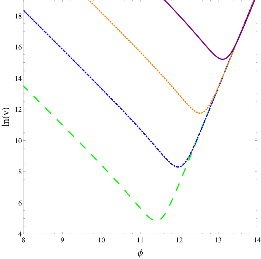
Finally, we point out that the energy density at the bounce can be made arbitrarily small by choice of scalar field momentum. As the value of $\pi_{\phi}$ is increased, the energy density at the bounce decreases. As mentioned earlier, this is one of the limitations of $\mu_{0}$ scheme in LQC which also holds in the presence of gauge-covariant flux modifications. This limitation is overcome in the $\bar{\mu}$-scheme discussed in the following where energy density at the bounce turns out to be a universal maximum.

To overcome limitations of $\mu_{0}$-scheme, the $\bar{\mu}$-scheme (also known as improved dynamics) was introduced in APS06c. Instead of adapting the regularization parameter to the fixed minimum area-eigenvalue, the $\bar{\mu}$-scheme adapts it with the physical area $p\bar{\mu}$ of a loop with $\Delta$. The regularization choice is:

$\displaystyle\bar{\mu}:=\sqrt{\Delta/|p|}$

(44)

While it was shown that this scheme has favorable physical properties, its implementation using LQG has not yet been established.⁸⁸ 8 In the full theory the regularization parameter is chosen to be a real number $\epsilon\in\mathbb{R}$ and not dependent on the phase space variables. This allowed the replacement of physical quantities inside Poisson brackets with their regulated analogs. As mentioned earlier, out of various possible regularizations it is only the $\bar{\mu}$-scheme which is known to be physically viable at ultra-violet and infra-red scales, and with physical predictions which are free from fiducial structures cs08. In other words, we are forced to implement the $\bar{\mu}$-scheme a posteriori after the regularized constraint $C^{\epsilon}[\tilde{N}]$ has been obtained. This is relevant for the case of study here, as the implementation of $\epsilon\to\bar{\mu}$ and the gauge-covariant flux corrections $p\to p\;{\rm sinc}^{2}(c\epsilon/2)$ do not commute. In this section we will hence study the constraint which arises, if one incorporates first the gauge-covariant flux corrections, i.e. $C^{\bar{\mu}}[\tilde{N}]$ from (26), or explicitly:

$$C^{\bar{\mu}}[\tilde{N}]=-\frac{6}{\kappa\gamma^{2}\Delta}\sin^{2}(c\bar{\mu})\sqrt{p}^{3}{\rm sinc}(c\bar{\mu}/2)+\frac{\pi_{\phi}^{2}}{2\sqrt{p}^{3}}{\rm sinc}^{-3}(c\bar{\mu}/2)~.$$

(45)

An important advantage of the $\bar{\mu}$-scheme in contrast to the earlier $\mu_{0}$ in standard LQC was that the bounce occurs at a universal value, $\rho_{\mathrm{b}}\approx 0.41\rho_{\mathrm{Pl}}$. Let us see whether this feature holds when modifications due to gauge-covariant fluxes are included. Using gauge-covariant expression for energy density $\rho:=\pi_{\phi}^{2}/(2p^{3}{\rm sinc}^{6}(\bar{\mu}c/2))$, the vanishing of the constraint (26) yields

$\displaystyle\rho=\frac{6}{\kappa\gamma^{2}\Delta}\sin^{2}(c\bar{\mu}){\rm sinc}^{-2}(c\bar{\mu}/2)$

(46)

whose maximum in $0<c\bar{\mu}<\pi$ is unique and can numerically be determined at $c\bar{\mu}\simeq 1.32419$ with $\rho_{\rm max}\simeq 0.515$, which is a bigger value compared to standard LQC. Thus, unlike $\mu_{0}$-scheme discussed earlier, quantum bounce occurs at the same value of energy density irrespective of the initial conditions.

References

- (1) T. Thiemann, Quantum Spin Dynamics (QSD): VII. Symplectic Structures and Continuum Lattice Formulations of Gauge Field Theories, Class. Quant. Grav. 18, 3293-3338 [arXiv:hep-th/00052232] (2001)
- (2) C. Rovelli, Quantum Gravity, Cambridge University Press (2004)
- (3) A. Ashtekar, J. Lewandowski, Background independent quantum gravity: A Status report, Class. Quant. Grav. 21, R53-R152 (2004)
- (4) T. Thiemann, Modern Canonical Quantum General Relativity, Cambridge University Press (2007)
- (5) R. Arnowitt, S. Deser, C. Misner, The Dynamics of General Relativity, In: Gravitation: An introduction to current research by L Witten (ed) New York 227-265 (1962)
- (6) A. Ashtekar, New variables for classical and Quantum Gravity, Phys. Rev. Lett.57, 2244-2247 (1986)
- (7) A. Ashtekar, New Hamiltonian formulation of General Relativity, Phys. Rev. D 36, 1587-1602 (1987)
- (8) J.F. Barbero, A real polynomial formulation of General Relativity in terms of connection, Phys. Rev. D 49, 6935-6938 (1994)
- (9) M. Bojowald, Loop Quantum Cosmology, Living Rev. Relativity 8, 11 (2005)
- (10) A. Ashtekar, P. Singh, Loop Quantum Cosmology: A Status Report, Class. Quant. Grav. 28, 213001 (2011)
- (11) A. Ashtekar, T. Pawlowski, P Singh, Quantum Nature of the Big Bang, Phys. Rev. Let. 96, 141301 (2006)
- (12) A. Ashtekar, T. Pawlowski, P. Singh, Quantum Nature of the Big Bang: An Analytical and Numerical Investigation, Phys. Rev. D 73, 124038 (2006)
- (13) A. Ashtekar, A. Corichi and P. Singh, Robustness of key features of loop quantum cosmology, Phys. Rev. D 77, 024046 (2008)
- (14) For a recent review of these developments see, I. Agullo, P. Singh, Loop Quantum Cosmology, in Loop Quantum Gravity: The First 30 Years, Eds: A. Ashtekar, J. Pullin, World Scientific (2017)
- (15) R. Gambini, J. Omedo and J. Pullin, Quantum black holes in loop quantum gravity, Class. Quant. Grav. 31, 095009 (2014).
- (16) A. Ashtekar, J. Olmedo and P. Singh, Quantum extension of the Kruskal spacetime, Phys. Rev. D 98, 126003 (2018)
- (17) J. Brunnemann. C Fleischhack, On the Configuration Spaces of Homogeneous Loop Quantum Cosmology and Loop Quantum Gravity, [arXiv:0709.1621] (2007)
- (18) C. Fleischhack, Kinematical Foundations of Loop Quantum Cosmology, [arXiv:1505.04400] (2015)
- (19) C. Beetle, J. Engle, M. Hogan, P. Mendonca, Diffeomorphism invariant cosmological symmetry in full quantum gravity, Int. J. Mod. Physics D 25, 1642012 (2016)
- (20) C. Beetle, J. Engle, M. Hogan, P. Mendonca, Diffeomorphism invariant cosmological sector in loop quantum gravity, [arXiv:1706.02424] (2017)
- (21) J. Engle, I. Vilensky, Deriving loop quantum cosmology dynamics from diffeomorphism invariance, [arXiv:1802.01543] (2018)
- (22) E. Alesci, F. Cianfrani, A new perspective on cosmology in Loop Quantum Gravity, [arXiv:1210.4504] (2012)
- (23) E. Alesci, F. Cianfrani, Quantum Reduced Loop Gravity: Semiclassical limit, [arXiv:1402.3155] (2014)
- (24) E. Alesci, G. Botta, G. Luzi, G Stagno, Bianchi I effective dynamics in Quantum Reduced Loop Gravity, [arXiv:1901.07140] (2019)
- (25) A. Dapor, K. Liegener, Cosmological Effective Hamiltonian from full Loop Quantum Gravity, Phys. Lett. B 785, 506-510 (2018)
- (26) A. Dapor, K. Liegener, Cosmological Coherent State Expectation Values in LQG I. Isotropic Kinematics, Class. Quant. Grav. 35, 135011 [arXiv:1710.04015] (2018)
- (27) K. Liegener, R. Lukasz, Cosmological Coherent State Expectation Values in LQG II. Thiemann-regularized Hamiltonian, (to appear)
- (28) A. Ashtekar, A. Corichi, J. Zapata, Quantum theory of geometry: III. Non-commutativity of Riemannian structures, Class. Quant. Grav. 15, 2955-2972 (1998)
- (29) L. Freidel, D. Louapre, Ponzano-Regge model revisited I: Gauge fixing, observables and interacting spinning particles, Class. Quant. Grav. 21, 5685-5726 (2004)
- (30) A. Baratin, B. Dittrich, D. Oriti, J. Tambornino, Non-commutative flux representation for loop quantum gravity, Class. Quant. Grav. 28, 175011 (2010)
- (31) L. Freidel, M. Geiller, J. Ziprick, Continuous formulation of the Loop Quantum Gravity phase space, Class. Quant. Grav. 30, 085013 (2011)
- (32) V. Bonzom, B. Dittrich, Dirac’s discrete hypersurface deformation algebras, [arXiv:1304.5983] (2013)
- (33) B. Dittrich, M. Geiller, A new vacuum for Loop Quantum Gravity, [arXiv:1401.6441] (2015)
- (34) A. S. Cattaneo, A. Perez, A note on the Poisson bracket of 2d smeared fluxes in loop quantum gravity, [arXiv:1611.08394] (2016)
- (35) M. Dupuis, L. Freidel, F. Girelli, Discretization of 3d gravity in different polarizations, Phys. Rev. D 96, 086017 (2017)
- (36) L. Freidel, F. Girelli, B Shoshany, 2+1D Loop Quantum Gravity on the Edge, [arXiv:1811.04360] (2018)
- (37) E. Magliaro, A. Marciano, C. Perini, Coherent states for FLRW space-times in loop quantum gravity, Phys.Rev. D 83, 044029 (2011)
- (38) K. Liegener, P. Singh, Gauge-invariant bounce from quantum geometry, arXiv:1906.02759
- (39) T. Thiemann, Gauge Field Theory Coherent States (GCS): I. General Properties, Class. Quant. Grav. 18, 2025-2064 (2001)
- (40) T. Thiemann, O. Winkler, Gauge Field Theory Coherent States (GCS): II. Peakedness Properties, Class. Quant. Grav., 2561-2636 18 (2001)
- (41) T. Thiemann, O. Winkler, Gauge Field Theory Coherent States (GCS): III. Ehrenfest Theorems, Class. Quant. Grav., 4629-4682 18 (2001)
- (42) T. Thiemann, Complexifier coherent states for quantum general relativity, Class. Quant. Grav. 23, 2063-2118 (2006)
- (43) H. Sahlmann, T. Thiemann, O. Winkler, Coherent states for canonical quantum General Relativity and the infinite tensor product extension, Nucl. Phys. B 606, 401-440 (2001)
- (44) K. Giesel, T. Thiemann, Algebraic Quantum Gravity (AQG) II. Semiclassical Analysis, Class. Quant.Grav. 24 2499-2564 (2007)
- (45) A. Ashtekar, M. Bojowald and J. Lewandowski, Mathematical structure of loop quantum cosmology, Adv. Theor. Math. Phys. 7, 233 (2003)
- (46) A. Ashtekar, T. Pawlowski, P. Singh, Quantum Nature of the Big Bang: Improved dynamics, Phys. Rev. D 74, 084003 (2006)
- (47) K. Liegener, P. Singh, Some physical implications of regularization ambiguities in SU(2) gauge-invariant loop quantum cosmology [arXiv:1908.07543] (2019)
- (48) C. Rovelli, L. Smolin, Discreteness of area and volume in quantum gravity, Nucl. Phys. B 442, 593-622 (1995)
- (49) A. Ashtekar, J. Lewandowski, Quantum Theory of Gravity I: Area Operators, Class. Quant. Grav. 14, A55-A82 (1996)
- (50) A. Ashtekar, J. Lewandowski, Quantum Theory of Geometry II: Volume Operators, Adv. Theor. Math. Phys 1, 388-429 (1998)
- (51) T. Thiemann, Quantum Spin Dynamics (QSD) I, Class. Quant. Grav. 15, 839-873 (1998)
- (52) T. Thiemann, Quantum Spin Dynamics (QSD) II, Class. Quant. Grav. 15, 875-905 (1998)
- (53) J. Kogut, L Susskind, Hamiltonian Formulation of Wilsons Lattice Gauge Theories, Phys. Rev. D 11 (1975)
- (54) A. Corichi, P. Singh, Is loop quantization in cosmology unique?, Phys. Rev. D 78, 024034 (2008)
- (55) P. Diener, B. Gupt, P. Singh, Numerical simulations of a loop quantum cosmos: robustness of the quantum bounce and the validity of effective dynamics, Class. Quant. Grav. 31, 105015 (2014)
- (56) P. Diener, A. Joe, M. Megevand, P. Singh, Numerical simulations of loop quantum Bianchi-I spacetimes, Class. Quant. Grav. 34, 094004 (2017)
- (57) V. Taveras, Corrections to the Friedmann Equations from LQG for a Universe with a Free Scalar Field. Phys. Rev. D 78, 064072 (2008)
- (58) B. Li, P. Singh, A. Wang, Towards Cosmological Dynamics from Loop Quantum Gravity, Phys Rev. D 97, 084029 (2018)
- (59) A. Ashtekar, E. Wilson-Ewing, Loop quantum cosmology of Bianchi type II models, Phys. Rev. D 80, 123532 (2009)
- (60) E. Wilson-Ewing, Loop quantum cosmology of Bianchi type IX models, Phys. Rev. D 82, 043508 (2010)
- (61) A. Corichi, A. Karami, Loop quantum cosmology of k=1 FRW: A tale of two bounces, Phys. Rev. D 84, 044003 (2011)
- (62) A. Corichi, A. Karami, Loop quantum cosmology of k=1 FLRW: Effects of inverse volume corrections, Class. Quant. Grav. 31, 035008 (2014)
- (63) S. Saini, P. Singh, Generic absence of strong singularities in loop quantum Bianchi-IX spacetimes, Class. Quant. Grav. 36, 105014 (2019)
- (64) S. Saini and P. Singh, Von Neumann stability of modified loop quantum cosmologies, Class. Quant. Grav. 36, 105010 (2019)
- (65) P. Singh, E Wilson-Ewing, Quantisation ambiguities and bounds on geometric scalars in anisotropic loop quantum cosmology, Class. Quant. Grav. 31, 035010 (2014)
- (66) A Kolmogoroff, Zur Groessenordnung des Restgliedes Fourierscher Reihen Differenzierbarer Funktionen, Ann. of Math. 36, 521-526 (1935)
- (67) C. Barrera-Figueroa, A. Lucas-Bravo, J. Lopez-Bonilla, The remainder term in Fourier series and its relationship with the Basel problem, Ann. Math. et Info. 34, 17-28 (2007)
- (68) M. Bojowald, Loop Quantum Cosmology I: Kinematics, Class. Quant. Grav. 17, 1489-1508 (1999)
- (69) M. Bojowald, Loop Quantum Cosmology II: Volume Operators, Class. Quant. Grav. 17, 1509-1526 (1999)
- (70) J. Velhino, The Quantum Configuration Space of Loop Quantum Cosmology, Class Quant Grav. 24, 3745-3758 (2007)
- (71) M. Assanioussi, A. Dapor, K. Liegener, T. Pawlowski, Emergent de Sitter epoch of the quantum Cosmos: a detailed analysis. [arXiv:1906.05315] (2019)
- (72) L. Smolin, Did the Universe evolve? Class. Quant. Grav. 9, 173 (1992)
- (73) R. Gambini, J. Pullin, Discrete quantum gravity: A Mechanism for selecting the value of fundamental constants, Int. J. Mod. Phys. D 12, 1775 (2003)
- (74) P. Hasenfratz, Prospects for perfect actions, Nucl. Phys. Proc. Suppl. 63, 53-58 (1998)
- (75) P. Hasenfratz, The theorectical background and properties of perfect actions, [arXiv:hep-lat/9803027] (2008)
- (76) T. Lang, K. Liegener, T. Thiemann, Hamiltonian Renormalisation III: Renormalisation Flow of 1+1 dimensional scalar fields: Properties, Class. Quant. Grav. 35, 245013 (2018)
- (77) M. Assanioussi, Polymer quantization of connection theories: Graph coherent states, Phys. Rev. D 98, 045016 (2018)
- (78) T. Thiemann, A. Zipfel, Stable Coherent States, Phys. Rev. D 93, 084030 (2016)