String and conventional order parameters in the solvable modulated quantum chain
Abstract
The phase diagram and the order parameters of the exactly solvable quantum model are analysed. The model in its spin representation is the dimerized spin chain in the presence of uniform and staggered transverse fields. In the fermionic representation this model is the dimerized noninteracting Kitaev chain with a modulated chemical potential. The model has a rich phase diagram which contains phases with local and nonlocal (string) orders. We have calculated within the same systematic framework the local order parameters (spontaneous magnetization) and the nonlocal string order parameters, along with the topological winding numbers for all domains of the phase diagram. The topologically nontrivial phase is shown to have a peculiar oscillating string order with the wavenumber , awaiting for its experimental confirmation.
I Introduction
According to the Landau theory, phases are distinguished by different types of long-ranged order, or its absence. The order is described by an appropriately chosen order parameter, understood implicitly as a local quantity. Landau5 There is a quite large number of examples of low-dimensional fermionic or spin systems as chains, ladders, frustrated magnets, topological and Mott insulators, etc, FradkinBook13; TI; Ryu10; Montorsi12; HiddenSSB; SOPladders; Kitaev06; Delgado; Kim; UsLadd; KitHeis2019 (and more references in there) which clearly manifest distinct phases, criticality, but lack conventional local order even at zero temperature.
In the related recent work we have systematically demonstrated how the Landau formalism can be extended to deal with nonconventional quantum orders. GT2017; GYC2018 The key point is to incorporate nonlocal string operators, denNijs89 string correlation functions, and string order parameters (SOPs). The appearance of nonlocal SOP is accompanied by a hidden symmetry breaking. HiddenSSB The local and nonlocal order parameters are related by duality, GT2017; GYC2018; Kogut79; ChenHu07; Xiang07; Nussinov and it is eventually a matter of choice of variables of the Hamiltonian.
There are some additional aspects of quantum order quantified by, e.g., winding or Chern numbers, Berry phases, concurrence, entanglement, FradkinBook13 which are not reducible to the parameters of the conventional Landau theory. These quantities provide rather complementary description and do not seem to be indispensable. GT2017; GYC2018
Nonlocal order parameters are known to be instrumental to probe hidden orders in various low-dimensional systems SOPladders; Delgado; Kim; KitHeis2019; GT2017; GYC2018; ChenHu07; Xiang07; Nussinov; Berg08; Rath13. A SOP naturally becomes a part of the Landau paradigm, since its critical index satisfies the standard scaling relations known for conventional order parameters GT2017; GYC2018, and thus can be used to determine the universality class of a given transition. The challenges in dealing with SOP are two-fold: from the theoretical side, in most of cases, this parameter quantitatively can be obtained via some arduous simulations. Experimentally, the string correlation functions are notoriously hard to measure. However, in the light of recent reports on experimental observation of bosonic string order, Enders11 one can expect more progress in observation of SOPs in the near future.
In the context of said hurdles, it is really important to gain more insight on SOPs by dealing with rather simple but nontrivial models. The model we study, in the guise of the dimerized chain with homogeneous and alternating transverse fields has been known for several decades. Perk75 It is exactly solvable, and its spectrum and phase diagram are well known. Perk75; TIMbook However, the explicit calculations for the spontaneous magnetization seem to be missing in the literature. More importantly, the nature of the order in the topological phase was not clarified, and here we report our finding of its nonlocal string order, modulated with the wavevector . The model in its fermionic representation is the Kitaev chain Kitaev2001 of noninteracting fermions with dimerized hopping and modulated (chemical) potential. The solvable Kitaev models with dimerizations and spatial modulations of potential were studied very actively in recent years with the focus on their topological phases with hidden orders and Majorana edge states DeGottardi11; Lang12; Cai; EzawaNagaosa14; Zeng16; Miao17a; Ezawa17; Miao17b; Ohta16; Ghadimi17; Katsura; Monthus18; Wang18; GYC2018 In the context of current research interest, the present model provides a nice exactly solvable example with rich critical properties, when the phase diagram contains both conventional local and quite peculiar nonlocal orders.
The rest of the paper is organized as follows: In Sec. II we introduce the spin and fermionic representations of the model. We also discuss its spectrum, phase diagram, and the field-induced magnetization. Sec. III contains the results. We present the formalism, the calculation of the spontaneous magnetization (local order parameter) for the magnetic phase, the string order parameter for the topological phase, and the winding numbers. The Appendices contain details on the Majorana representations of the Hamiltonian and additional technical information on the string operators and string order parameters. The results are summarized and discussed in the concluding Sec. IV.
II Model
II.1 Spin and fermionic representations of the model
In this subsection we define the model and recapitulate its main results known explicitly or implicitly from earlier work. The spin Hamiltonian of the model is the dimerized quantum chain in the presence of uniform () and alternating () transverse magnetic fields:
| (1) |
Here -s are the standard Pauli matrices, is the nearest-neighbor exchange coupling, and and are the anisotropy and dimerization parameters, respectively. This exactly-solvable model was first introduced and analyzed by Perk et alPerk75. (See also DelGamMod; Lima; Sen2008; GT2017 for related more recent work on versions of this model.) The standard Jordan-Wigner (JW) transformation Lieb61; Franchini2017 maps (1) onto the free-fermionic Hamiltonian
| (2) |
called in recent literature the (modulated) Kitaev chain.Kitaev2001 In the fermionic representation (2) the chain has dimerized hopping and modulated chemical potential. So, whether we deal with the modulated spin or the Kitaev fermionic chains, is a matter of mere convention, especially since the results below will be given in terms of spins or fermions, on the same footing.
The duality transformation is defined as Perk; Fradkin78
| (3) | |||||
| (4) |
where obey the standard algebra of the Pauli operators and reside on the sites of the dual lattice which can be placed between the sites of the original chain. This transformation maps (1) onto the dual spin Hamiltonian
| (5) | |||
| (6) | |||
| (7) | |||
| (8) |
which is a sum of two 1D transverse Ising models residing on the even and odd sites of the dual lattice, plus the field-induced symmetry-breaking term which couples the even and odd sectors of the dual -Hamiltonian.
II.2 Spectrum
The Hamiltonian (2) can also be written as
| (9) |
where the fermions are unified in the spinor
| (10) |
with the wavenumbers restricted to the reduced Brillouin zone (BZ) and we set the lattice spacing . The band index serves to map the JW fermions from the full -periodic BZ onto the reduced zone as
| (11) |
where is the Heaviside step function. The JW fermion in the coordinate representation (2) is:
| (12) |
The Hamiltonian matrix (we set from now on) can be written as
| (13) |
with
| (14) |
and
| (15) |
The Hamiltonian has four eigenvaluesPerk75 where
| (16) |
with
| (17) |
and
| (18) |
II.3 Phase diagram
The phase diagram of the model was first found by Perk et alPerk75. See also TIMbook for a recent review. The critical lines where the model becomes gapless are determined by the condition . Cf. eqs. (16), (18) and Fig. 1.

There are three phase boundaries:
(i) at
| (19) |
the gap vanishes at the center of the BZ ().
(ii) At the edge of the BZ () the gap vanishes on the circle
| (20) |
(iii) Two critical line segments at correspond to the gap vanishing at the incommensurate (IC) wavevector
| (21) |
The IC solution exists in the range of parameters:
| (22) |
The wavevector (21) varies continuously from at the intersection of and to where the critical segments end at the intersections with the circle.
It is useful to plot the phase boundary (20) in the plane, especially keeping in mind connection to the earlier work GT2017. This phase diagram is shown in Fig. 2.

II.4 Field-induced magnetizations
Differentiation of the free energy with respect to and to yields magnetizations
| (23) |
and
| (24) |
respectively.Perk75 At zero temperature the explicit expressions are:
| (25) |
and
| (26) |
where we defined the auxiliary parameters:
| (27) |
The physics becomes more transparent if we introduce two magnetizations on even/odd sublattices as
| (28) |
We plot all four field-induced magnetizations as functions of the uniform component of the magnetic field in Fig. 3. Two cases need to be distinguished. The first case shown in panel (a) corresponds to the variation of the field along the path on the phase diagram in the plane shown in Fig. 1. The path crosses the PM-FM phase boundary at and the boundary between the ferromagnetic and topological phases at . The magnetizations have noticeable cusps at these critical points, which after differentiation result in divergent susceptibilities.Perk75 At the intermediate field (its value is available numerically only) the odd sublattice magnetization vanishes and the induced magnetic pattern changes from ferrimagnetic to antiferrimagnetic (see Fig. 4). This point is not related to any singularities in magnetizations or their derivatives.
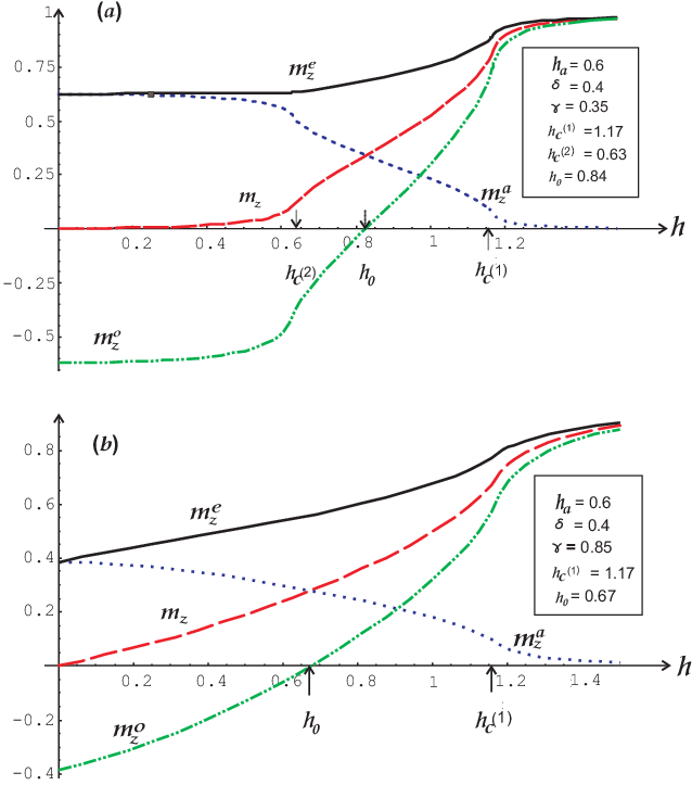
The second case shown in panel (b) corresponds to the path on the phase diagram. It crosses only the PM-FM phase boundary and bypasses the topological phase. The magnetizations demonstrate cusps at the only critical point , while at , including the point of the induced pattern switch, the magnetizations and their derivatives are analytical.

The main conclusions following from the analysis of the field-induced magnetization are: (i) the magnetization cusps which translate into corresponding diverging susceptibilities do probe the critical points (phase boundaries); (ii) the vanishing odd sublattice magnetization and related change of direction of the odd magnetization at the intermediate field do not constitute a critical point; (iii) the components of transverse magnetization cannot probe the order (or serve to build up a local order parameter) of the phase lying inside the circle shown in Fig. 1.
III Order Parameters
III.1 Bogoliubov tranformation and Majorana operators
To diagonalize the Hamiltonian (9) in terms of the new fermionic operators , we utilize the Bogoliubov canonical transformation within the formalism worked out in Lieb61; Lima. It is convenient to introduce the Majorana fermions as
| (29) |
Then the Bogoliubov transformation reads as
| (30) | |||||
| (31) |
The unitary matrices and
| (32) |
are constructed from the normalized (left) eigenvectors of the operators whose eigenvalues are . Explicitly, and solve the following equations:
| (33) | |||||
| (34) |
where
| (35) |
In addition, these matrices satisfy the conditions:
| (36) | |||||
| (37) |
We find
| (38) |
where
| (39) |
and
| (40) |
with
| (41) |
One can also parameterize in terms of the Bogoliubov ange defined as
| (42) |
Once the solution of (33) is found, the solution of (34) can be calculated straightforwardly as
| (43) |
(Alternatively, one can first find from (34), and then as .) Using the thermodynamic average for the Bogoliubov fermions
| (44) | |||||
| (45) |
where is the Fermi-Dirac distribution function, we can obtain the field-induced magnetization
| (46) |
The above formula is equivalent to Eq. (25) obtained from differentiation of the partition function. Introducing the matrix
| (47) |
we find the zero-temperature correlation function of the Majorana operators:
| (48) |
The explicit form of matrix (47) is calculated from Eqs. (38), (43). One can check that its components satisfy the following relations:
| (49) | |||||
| (50) |
Then Eq. (48) can be simplified into
| (51) |
where the matrix elements are found to be:
| (52) | |||||
| (53) |
The formulas derived in this subsection provide us with the main results needed for the rest of calculations.
III.2 Spontaneous magnetization
We define the spontaneous longitudinal sublattice magnetizations as
| (54) | |||||
| (55) |
The spontaneous longitudinal magnetization is the (local) order parameter defined as
| (56) |
We also define the Majorana string operator:
| (57) |
(By definition .) For further reference let us remind some useful relations between original spins, Majorana fermions, and the dual spin operators (3,4):
| (58) | |||||
| (59) |
Then . The spin-correlation function can be calculated as the correlation function of the Majorana string operators: Lieb61
| (60) |
The latter is given by the determinant:
| (61) |
To calculate the quantities of our interest we choose the ends as:
| (62) |
In both cases we are dealing with matrices. Note that (61) is not the Toeplitz determinant, since the elements of the matrix given by Eq.(51) do not satisfy the condition . It is however possible to represent (61) via the block Toeplitz matix. Widom70; Basor2019 Let us define
| (63) |
and its inverse Fourier transform
| (64) |
along with the matrix
| (65) |
Then the sublattice magnetizations can be evaluated as the limit of the determinant of the corresponding block Toeplitz matrix constructed from blocks of size :
| (66) |
At this point we were unable to derive analytical results for asymptotics of the above block Toeplitz determinants. So we resort to direct numerical calculations for large finite-size matrices. The results for spontaneous magnetization are given in Fig. 6. The numerical values of the parameters we present in that figure are stable in the fourth decimal place for the matrices of sizes . In immediate vicinities of the critical points the order parameters are checked to decay smoothly as .
We checked that the numerical results obtained from (66) agree with two available analytical limits at .
| (67) |
For the result is due to Pfeuty: Pfeuty70
| (68) |
For the case the order parameter can be obtained by combining the result of Pfeuty and the duality transformations (3) and (4), yielding GT2017
| (69) |
The analytical results (68) and (69) can be obtained from (66) by the brut force calculations utilizing Szegö’s theorem McCoyBook, but those calculations are quite demanding, see Appendices for more details.
The expressions for are obtained along the same lines. Numerical values satisfy useful relation , see Fig. 6.
III.3 Nonlocal string order
We define another string operator
| (70) |
and the related string correlation function:
| (71) |
Inside the circle this string correlation function is found to be oscillating with the period of four lattice spacing, see Fig. 5, so we will label it as -phase to distinguish it from the positive “ferrimagnetic-like” string correlation function in the paramagnetic phase .

We will need three parameters to account for the string order:
| (72) |
The reason for this is that due to the dimerization and the staggered field , the value of the string correlation function depends not only on the length of the string, but also on whether its ends are sitting on the even or odd sites of the chain. The explicit matrix form (71) with the elements can be written as the block Toeplitz matrix, similar to (66). Four-site periodic oscillations of the string correlation function inside the circle indicate periodicity of orientations of spins along the string, or, alternatively, the modulation of fermionic density around half-filling. In the FM phase (see Fig. 1) the string correlation function vanishes at large length, while in the paramagnetic phase it is positive, showing only quite trivial “ferrimagnetic” oscillations synchronized with the staggered field. Qualitatively, it indicates that all spins in the string are polarized along the field, or, in terms or fermions, the latter have concentration above half-filling.
In the limit the hyperbolic phase boundaries shown in Fig. 2 reduce to two lines , GT2017 and nonvanishing SOPs are localized inside the cone . When the only surviving component of the 4-periodic string correlation function is , such that
| (73) |
while . Similarly, when
| (74) |
while . Note useful relations:
| (75) | |||||
| (76) |
In the limit the averaging of the even and odd strings decouples, and the SOPs can be found in a simple form. The values inside the cone are available GT2017 yielding
| (77) |
We have checked the agreement between the analytical result (77) and the numerical evaluation of the determinant (71).

III.4 Winding Number
It has been shown in recent years that many quantum phase transitions with hidden orders are accompanied by a change of topological numbers FradkinBook13; TI. Here we calculate the winding number (or the Pontryagin index) in all regions of the model’s phase diagram. Such parameters were calculated recently in similar 1D models, see, e.g., Wu12; Niu12; EzawaNagaosa14; Zeng16; GT2017; Ezawa17; Miao17b
By a unitary transformation the Hamiltonian (13) can be brought to the block off-diagonal form
| (78) |
with the operator
| (79) |
which has two eigenvalues
| (80) |
In one spatial dimension the winding number defined as SchnyderRyu11
| (81) |
can be readily calculated for this model as:
| (82) |
The results for are given on the ground-state phase diagram in Fig. 1. can be viewed as a complimentary parameter characterizing a given phase. The disordered (PM) phase and the magnetic phases where conventional local order exists, are topologically trivial, . The phase inside the circle where modulated nonlocal string order parameter exists, is topologically nontrivial, .
IV Conclusion
The main motivation for this work was to further advance the framework incorporating nonlocal string order into an “extended” Landau paradigm. For a large class of quantum spin or fermionic problems we are interested in, the effective Ginzburg-Landau Hamiltonian to deal with, is a quadratic fermionic Hamiltonian. In general such a Hamiltonian is already a result of some mean-field approximation, UsLadd; GT2017 but there is a considerable number of physically interesting problems where it is the microscopic Hamiltonian of the model. Postponing for future work building up the very important element – the Wilsonian renormalization group appproach to systematically deal with the nonlocal order beyond the mean field, we chose a non-interacting fermionic model to analyze.
The model is the dimerized Kitaev chain with modulated chemical potential, which was initially introduced and studied Perk75 as the dimerized spin chain in the uniform and staggered transverse fields. These are two equivalent representations of the model, since they map onto each other via the Jordan-Wigner transformation. This relatively simple model is very relevant for studies of quantum critical and out-of-equilibrium properties. TIMbook The model has a rich phase diagram (see Fig. 1) which contains phases with local magnetic and nonlocal modulated string orders.
We have calculated the sponataneous magnetizations (local order parameters) showing that they smoothly vanish at the corresponding phase boundaries via second-order quantum phase transitions. (Despite the fact that the model was studied before, Perk75; Lima; Sen2008; TIMbook we could not find the explicit results for magnetization in the previous literature.) For the first time we have established the nature of the order in the topological phase lying inside the circle in Fig. 1. In that phase the modulated string order appears via a second-order phase transition. The modulations are signalled by the oscillations of the string-string correlation function with the wave number . Physically, this correlation function probes the average of the string made out of spins, or, equivalently, the string of fermionic density operators (with respect to half-filling). In addition, we have calculated the winding number in all phases. The disordered (PM) phase and the A(FM) phase with conventional local order parameter are topologically trivial, , while the phase with the modulated string order has . Form the results for the gaps and the free-fermionic nature of the model we infer its critical indices to belong to the 2D Ising universality class. Note
We need to stress once again GT2017; GYC2018 that there is no insurmountable difference between the local and string order parameters. Using judiciously chosen duality transformations we show that a SOP can be identified as a local order parameter of some dual Hamiltonian. Sometimes this can help to easily calculate the SOP in the dual framework, GT2017; GYC2018, sometimes not. But it is important to understand as a matter of principle. For the general case when all model’s parameters are nonzero we were able to define the duality transformations reducing the SOPs to local “dual” orders, but it did not result in technical simplifications in the calculations of SOPs.
On the technical side, the framework we present is quite straightforward: One needs to solve the problem of the Bogoliubov transformation which allows to find explicit expression for the two-point Majorana correlation functions. The latter are building blocks of the Toepliz matrices. The local and string order parameters, regardless of the original spin or fermionic representations, are given by the asymptotes of the corresponding Majorana string correlation functions. The calculations of local and nonlocal parameters are reduced to the well-defined mathematical problem of the evaluation of limits of determinants of the (block) Toeplitz matrices. These matrices are found in a closed form in terms of the two-point Majorana correlation functions. With some luck and skills these limits can be found explicitly, McCoyBook then one gets algebraic expressions for the order parameters. In this paper we found several expressions for the order parameters for particular limits of the model’s couplings. For the general case we were unable to do so. The generalization of Szegö’s theorem for the block Toeplitz matrices appeared to be a quite challenging mathematical problem. Widom70; Basor2019 This is however a simple numerical calculation, NoteMath and our numerical results are summarized in Fig. 6.
A very promising development of our results would be to find realizations of this model to experimentally detect the predicted modulated string order. Very interesting questions of the IC gapless phase, disorder lines and the Majorana edge states in this model will be addressed in a separate work.
Acknowledgements.
G.Y.C. thanks the Centre for Physics of Materials at McGill University, where this work was initiated, for hospitality. We are grateful to J.H.H. Perk for bringing important papers to our attention and to Y.Y. Tarasevich for helpful comments. Financial support from the Laurentian University Research Fund (LURF), the Ministry of Education and Science of the Russian Federation (state assignment grant No. 3.5710.2017/8.9), is gratefully acknowledged.Appendix A Separation of the Majorana Hamiltonian.
In the main text of the paper we kept definitions and transformations consistent with those of earlier related work GT2017; GYC2018 to preserve continuity in the series. In this Appendix we will use some modified transformations which make the analysis of separability of the Hamiltonian, analytical treatment of its limiting cases, and the symmetry, more transparent. To this end we introduce two new species of Majorana fermions (compare to (29)) as
| (83) |
Then the JW and duality transformations (3,4) read: (compare to (58) and (59))
| (84) | |||||
| (85) |
This transformation maps the original Hamiltonian (1) (cf. also (5)-(8)) onto
| (86) | |||||
| (87) | |||||
| (88) | |||||
| (89) |
Recombining two Majorana fermions into a (new) single JW fermion as
| (90) |
and Fourier-transforming it according to (with or for or , resp.), we can bring the Hamiltonian into the spinor form (9) with
| (91) |
and
| (92) |
Here
| (93) |
and
| (94) |
In the limit the off-diagonal block . Then the averaging in the even and odd sectors decouples, and the correlation functions of the even/odd Majorana operators can be evaluated independently. One can check from the above formulas that these quantities can be calculated from the Toeplitz matrices with the generating functions of their elements given by the standard expressions known from the solution of the Ising chain in transverse field.McCoyBook Unfortunately, when such technical simplification is no longer available.
A unitary transformation
| (95) |
brings the spinor (91) into the new form
| (96) |
The transformed Hamiltonian matrix (92)
| (97) |
is brought to the form (13) with the new matrices and . The rest can be done along the lines of the analysis presented in the main text. We will not however elaborate further and present more results on this formalism, since it did not give us a clear advantage in dealing with the case .
Appendix B String operators , and their correlation functions
In addition to the string (57) one can define the even and odd string operators:GYC2018
| (98) | |||||
| (99) | |||||
In the above formulas we used the second auxiliary set of the Majorana operators (distinguished by tildes) defined by (83). These operators are very insightful for dealing with the even and odd sectors of the Majorana Hamiltonian (86). The string operators (98) and (99) are also presented in terms of the dual spins using (58) and (84). The Majorana string operator (57) is related to the above operators as
| (100) |
The even/odd SOPs () are introduced as
| (101) |
From (58), (98), (99) one can establish an important relation GT2017; GYC2018 between the nonlocal even/odd SOPs and the local dual sublattice magnetizations of the dual spins:
| (102) |
if the parity of and is chosen in agreement with (62). Another operator’s identity
| (103) | |||||
allows to establish an important physical property: the spontaneous magnetization of “original” spins is due to overlap of the even and odd SOPs.NoteSig-O-tau In the absence of coupling between the even and odd sectors of the Hamiltonian (8) when , the above identity results in GT2017
| (104) |
and Eq. (69) as a consequence. When the factorization of the contributions from the even and odd sectors does not occur.
The even and odd SOPs are numerically calculated from the determinant of the ordinary Toeplitz matrix:
| (105) |
To probe additional nonlocal orders we utilize another pair of string operators:GYC2018
| (106) | |||||
| (107) | |||||
The corresponding SOPs are defined similarly to (101) NoteOy and are numerically calculated from the following Toeplitz determinant:
| (108) |
One can establish relation GT2017; GYC2018; NoteOy between the nonlocal SOPs and the sublattice magnetization of the dual spins:
| (109) |
Similarly to the results of subsection B, the spontaneous magnetization of the original spins can be determined from the correlation function of the string operator , cf. (60).
In the limit the above determinants can be evaluated exactly by the standard technique, McCoyBook reproducing the earlier results for nonvanishing obtained from duality mappings.GT2017 When and/or we were unable to derive analytical results for asymptotics of these Toeplitz determinants. Numerical results show that in the presence of fields all SOPs die off in the thermodynamic limit . So the only nonvanishing SOP is discussed in the main text. Similarly to the results (102) and (109) yielding a simple local dual interpretation of the SOPs and , the duality transformation (3,4) with the interchange brings the SOP to the long-ranged order of the dual spins. We emphasize this possibility to map the string order onto a local order in terms of some judiciously chosen dual variables. We will not go into mathematical details for the case of , since it is not useful at this point for getting analytical results.
References
- (1) L.D. Landau and E.M. Lifshitz, Statistical Physics Part 1. Course of Theoretical Physics Vol. 5 , 3rd ed., (Butterworth-Heinemann, Oxford, 1980).
- (2) E. Fradkin, Field Theories of Condensed Matter Physics, 2nd edition (Cambridge University Press, New York, 2013).
- (3) B.A. Bernevig and T.L. Hughes, Topological Insulators and Topological Superconductors (Princeton University Press, Princeton, 2013).
- (4) S. Ryu, A.P. Schnyder, A. Furusaki, and A.W.W. Ludwig, New J. Phys. 12, 065010 (2010).
- (5) A. Montorsi and M. Roncaglia, Phys. Rev. Lett. 109, 236404 (2012).
- (6) M. Oshikawa, J. Phys. Condens. Matt. 4, 7469 (1992); T. Kennedy and H. Tasaki, Phys. Rev. B 45, 304 (1992); M. Kohmoto and H. Tasaki, Phys. Rev. B 46, 3486 (1992).
- (7) H. Watanabe, Phys. Rev. B 52, 12508 (1995); Y. Nishiyama, N. Hatano and M. Suzuki, J. Phys. Soc. Jpn. 64, 1967 (1995); D. G. Shelton, A. A. Nersesyan, and A. M. Tsvelik, Phys. Rev. B 53, 8521 (1996).
- (8) A. Kitaev, Ann. Phys. 321, 2 (2006).
- (9) M.A. Martin-Delgado, R. Shankar, and G. Sierra, Phys. Rev. Lett. 77, 3443 (1996); M.A. Martin-Delgado, J. Dukelsky, and G. Sierra, Phys. Lett. A 250, 430 (1998); J. Almeida, M.A. Martin-Delgado, and G. Sierra, Phys. Rev. B 76, 184428 (2007); ibid 77, 094415 (2008); J. Phys. A 41, 485301 (2008).
- (10) E.H. Kim, G. Fath, J. Solyom, and D. J. Scalapino, Phys. Rev. B 62, 14965 (2000); G. Fath, O. Legeza, and J. Solyom, Phys. Rev. B 63, 134403 (2001); E.H. Kim, O. Legeza, and J. Solyom, Phys. Rev. B 77, 205121 (2008).
- (11) S.J. Gibson, R. Meyer, and G.Y. Chitov, Phys. Rev. B 83, 104423 (2011); G.Y. Chitov, B.W. Ramakko, and M. Azzouz, Phys. Rev. B 77, 224433 (2008); M. Azzouz, K. Shahin, and G.Y. Chitov, Phys. Rev. B 76, 132410 (2007).
- (12) A. Catuneanu, E.S. Sørensen, and H.-Y. Kee, Phys. Rev. B 99, 195112 (2019); C.E. Agrapidis, J. van den Brink, and S. Nishimoto, Phys. Rev. B 99, 224418 (2019).
- (13) G.Y. Chitov and T. Pandey, J. Stat. Mech. (2017) 043101.
- (14) G.Y. Chitov, Phys. Rev. B 97, 085131 (2018).
- (15) M. den Nijs and K. Rommelse, Phys. Rev. B 40, 4709 (1989).
- (16) J.B. Kogut, Rev. Mod. Phys. 51, 659 (1979).
- (17) H.-D. Chen and J. Hu, Phys. Rev. B 76, 193101 (2007).
- (18) X.-Y. Feng, G.-M. Zhang, and T. Xiang, Phys. Rev. Lett. 98, 087204 (2007).
- (19) H.-D. Chen and Z. Nussinov, J. Phys. A: Math. Theor. 41, 075001 (2008); E. Cobanera, G. Ortiz, and Z. Nussinov Phys. Rev. B 87, 041105(R) (2013).
- (20) E. Berg, E.G. Dalla Torre, T. Giamarchi, and E. Altman, Phys. Rev. B 77, 245119 (2008).
- (21) S.P. Rath, W. Simeth, M. Endres, and W. Zwerger, Annals of Physics 334, 256 (2013).
- (22) M. Endres, et al, Science 334, 200 (2011).
- (23) J.H.H. Perk, H.W. Capel, M.J. Zuilhof, and Th. J. Siskens, Physica A 81, 319 (1975).
- (24) A. Dutta, G. Aeppli, B.K. Chakrabarti, U. Divakaran, T.F. Rosenbaum, and D. Sen, Quantum Phase Transitions in Transverse Field Spin Models: From Statistical Physics to Quantum Information (Cambridge University Press, New Delhi, 2015).
- (25) A. Kitaev, Usp. Fiz. Nauk (Suppl.) 44, 131 (2001).
- (26) W. DeGottardi, D. Sen, and S. Vishveshwara, New J. Phys. 13, 065028 (2011); Phys. Rev. Lett. 110, 146404 (2013).
- (27) L.-J. Lang and S. Chen, Phys. Rev. B 86, 205135 (2012).
- (28) X. Cai, L.-J. Lang, S. Chen, and Y. Wang, Phys. Rev. Lett. 110, 176403 (2013); X. Cai, J. Phys.: Condens. Matter 26, 155701 (2014).
- (29) R. Wakatsuki, M. Ezawa, Y. Tanaka, and N. Nagaosa, Phys. Rev. B 90, 014505 (2014).
- (30) Q.-B. Zeng, S. Chen, R. Lü, Phys. Rev. B 94, 125408 (2016).
- (31) J.-J. Miao, H.-K. Jin, F.-C. Zhang, and Y. Zhou, Phys. Rev. Lett. 118, 267701 (2017).
- (32) M. Ezawa, Phys. Rev. B 96, 121105(R) (2017).
- (33) Y. Wang, J.-J. Miao, H.-K. Jin, and S. Chen, Phys. Rev. B 96, 205428 (2017).
- (34) T. Ohta and K. Totsuka, J. Phys. Soc. Jpn. 85, 074003 (2016).
- (35) R. Ghadimi, T. Sugimoto, and T. Tohyama, J. Phys. Soc. Jpn. 86, 11407 (2017).
- (36) H. Katsura, D. Schuricht, and M. Takahashi, Phys. Rev. B 92, 115137 (2015); K. Kawabata, R. Kobayashi, N. Wu, and H. Katsura, Phys. Rev. B 95, 195140 (2017).
- (37) C. Monthus, J. Phys. A: Math. Theor. 51, 465301 (2018)
- (38) Y. Wang, Phys. Rev. E 98, 042128 (2018).
- (39) F. Ye, G.-H. Ding, and B.-W. Xu, Commun. Theor. Phys. (Beijing, China) 37, 492 (2002); F. Ye and B.-W. Xu, Commun. Theor. Phys. (Beijing, China) 39, 487 (2003).
- (40) J.P. de Lima, L.L. Gonçalves, and T.F.A. Alves, Phys. Rev. B 75, 214406 (2007).
- (41) U. Divakaran, A. Dutta, and D. Sen, Phys. Rev. B 78, 144301 (2008).
- (42) E.H. Lieb, T. Schultz, and D. Mattis, Ann. Phys. (N.Y.) 16, 407 (1961).
- (43) F. Franchini, An Introduction to Integrable Techniques for One-Dimensional Quantum Systems, Lecture Notes in Physics 940, (Springer, Heidelberg, 2017).
- (44) H.W. Capel and J.H.H. Perk, Physica A 87, 211 (1977). For more literature and a recent overview on such transformation and dual -cluster Hamiltonians, see J.H.H. Perk, arXiv:1710.03384.
- (45) E. Fradkin and L. Susskind, Phys. Rev. D 17, 2637 (1978).
- (46) H. Widom, Adv. Math. 21(1), 1 (1976).
- (47) E. Basor, J. Dubail, T. Emig, and R. Santachiara, J. Stat. Phys. 174, 28 (2019)
- (48) P. Pfeuty, Ann. Phys. (N.Y.) 57, 79 (1970).
- (49) B.M. McCoy, Advanced Statistical Mechanics (Oxford University Press, New York, 2010).
- (50) N. Wu, Phys. Lett. A 376, 3530 (2012).
- (51) Y. Niu, S. B. Chung, C.-H. Hsu, I. Mandal, S. Raghu, and S. Chakravarty, Phys. Rev. B 85, 035110 (2012).
- (52) A.P. Schnyder and S. Ryu, Phys. Rev. B 84, 060504(R) (2011).
- (53) The exception is the IC critical line when . It belongs to the different universality class of the conformal charge . (The Ising belongs to the class).
- (54) In this work we used Mathematica to calculate block Toeplitz determinants. It takes about 1-2 minutes per point for matrix size.
- (55)
A similar identity can be derived for the spins on even sites:
- (56) In analytical work it is not convenient to deal with as strings of dual spins (106), (107). Instead,GT2017 it is easier to apply the duality transformations (3,4) with the interchange . Then the r.h.s. of Eqs. (106) and (107) become and , respectively.