Disorder driven multifractality transition in Weyl nodal loops
Abstract
The effect of short-range disorder in nodal line semimetals is studied by numerically exact means. For arbitrary small disorder, a novel semimetallic phase is unveiled for which the momentum-space amplitude of the ground-state wave function is concentrated around the nodal line and follows a multifractal distribution. At a critical disorder strength, a semimetal to compressible metal transition occurs, coinciding with a multi- to single-fractality transition. The universality class of this critical point is characterized by the correlation length and dynamical exponents. At considerably higher disorder, an Anderson metal-insulator transition takes place. Our results show that the nature of the semimetallic phase in non-clean samples is fundamentally different from a clean nodal semimetal.
The robustness of certain material properties to perturbations is arguably the most appealing property of topological matter. Topological insulators stood out as an important class of topological materials (Hasan and Kane 2010; Qi and Zhang 2011) whose stability with respect to interactions and disorder is by now fairly well established (Chiu et al. 2016; Rachel 2018). Gapless systems can, however, also support non-trivial momentum-space topology and are expected to be less robust to such effects. Among these, are the Weyl nodal loop (WNL) semimetals, for which the valence and conduction bands linearly touch along one-dimensional (1D) loops in the three-dimensional (3D) momentum space (Armitage et al. 2018). Their recent theoretical prediction (Kim et al. 2015; Weng et al. 2015; Mullen et al. 2015) and experimental discovery (Xie et al. 2015; Bian et al. 2016) triggered intense experimental (Schoop et al. 2016; Okamoto et al. 2016; Hu et al. 2016; Hu et al. 2017; Xu et al. 2017a; Lou et al. 2018; Laha et al. 2019; Qiu et al. 2019; Sims et al. 2019; Nakamura et al. 2019) and theoretical interest (Rhim and Kim 2015; Fang et al. 2015; Huang et al. 2016; Chan et al. 2016; Lu et al. 2017; Xu et al. 2017b; Du et al. 2017; Liu and Balents 2017; Oroszlány et al. 2018; Martín-Ruiz and Cortijo 2018; Wang et al. 2018; Lau and Ortix 2019; Ezawa 2019).
A manifestation of WNL’s topological nature is the presence of surface (“drumhead”) edge states (Burkov et al. 2011; Chen et al. 2015; Weng et al. 2015; Chan et al. 2016; Zhang et al. 2016) on surfaces parallel to the loop plane, which are induced by chiral symmetry. Since the Fermi surface is reduced to a 1D nodal line, the density of states (DOS), , vanishes linearly for low energies, i.e. .
The robustness of the topological semimetal state to interactions (Sur and Nandkishore 2016; Nandkishore 2016; Roy 2017; Shapourian et al. 2018; Araújo and Li 2018) and disorder (Syzranov and Skinner 2017; Chen et al. 2019) is of major importance to understand in which conditions it might be observed. For Dirac/Weyl systems with isolated nodal points, the effect of static disorder has recently been addressed by a series of thorough numerical studies (Pixley et al. 2015; Pixley et al. 2016a; Pixley et al. 2016b; Buchhold et al. 2018). The clean-limit incompressible semimetallic state was shown to survive up to a finite critical strength of a box-distributed disorder potential where a transition to a compressible diffusive metal takes place 11 1 For Gaussian distributed disorder, rare region effects were proposed to add a finite spectral weight at zero energy, causing an avoided quantum critical point (Pixley et al. 2016b). However, these effects were shown to add finite spectral weight only in the neighborhood of , not affecting the finite-disorder semimetallic phase (Buchhold et al. 2018).
For a WNL, the exact nature of the finite disorder state is yet unknown. Coulomb interactions were shown to induce a quasiparticle lifetime vanishing quadratically with the excitation energy, thus yielding Fermi liquid behavior (Huh et al. 2016). Weak disorder does not change the compressibility, to leading order (Wang and Nandkishore 2017). Nevertheless, disorder, with or without interactions, was found to be marginally relevant in the clean case (Wang and Nandkishore 2017), pointing to a different scenario than nodal point semimetals. Perturbative arguments are, however, of limited use to characterize the stable fixed point at finite disorder strength. The latter is of key importance to understand the properties of WNL compounds, particularly with regard to transport, which has, up to know, been assumed diffusive (Mukherjee and Carbotte 2017).

In this Letter, we unveil the phase diagram of a WNL in the presence of short-range disorder using numerically exact methods. It includes a novel multifractal (MF) semimetallic (SM) phase, corresponding to the stable fixed point for weak disorder. Our main results are summarized in Fig. 1. We show that any small amount of disorder mixes all the Weyl states along the nodal line depicted in Fig. 1(a), and that the width of the wave function, , vanishes as the linear system size, , increases. The resulting state is fundamentally different from the clean one. Although the DOS still vanishes at the Fermi-level, i.e. , the momentum-space wave-function has a multifractal structure. The MF-SM phase survives up to a critical value of the disorder strength, where a transition to a single-fractal (SF) metallic (M) phase takes place. In this phase the system is a standard diffusive metal with a finite and loses system size dependence. At larger disorder strength, an Anderson metal-insulator transition occurs. The phase diagram is sketched in Fig. 1(b).
Model and Methods.—
We study a two-band model of a WNL on a cubic lattice with short-range disorder,
| (1) |
The first term describes a clean WNL, with a 3D Bloch vector, , with Pauli matrices acting on the orbital pseudo-spin indices , and . The second term is the disorder potential, where is a lattice site and , with random variables . The results presented hereafter are for , , and . This choice yields a single nodal line, arising for . The hopping anisotropy breaks unwanted degeneracies and ensures the system is generic within this class.
We characterize the spectral and wave function properties by a combination of numerical methods. To compute the DOS we use the kernel polynomial method (KPM) with an expansion in Chebyshev polynomials to order (Andelković et al. 2019; João and Lopes), reaching system sizes up to . To characterize the system’s lowest energy eigenstates, we use Lanczos exact diagonalization (ED).
The eigenstates’ structure is revealed by the generalized momentum-space inverse participation ratio (Pixley et al. 2018; Fu et al. 2018),
| (2) |
where is the eigenstate amplitude in the Bloch momentum state and orbital . The size dependence is characterized by a -dependent exponent, , defined in terms of the generalized dimension, , as . In a ballistic phase, the wave function is localized in momentum space, does not change with and for . For a 3D-diffusive metal or an Anderson insulator, . In these cases is constant, and the system is a single-fractal. Multifractals correspond to cases where is -dependent. This happens, for instance, for the real-space inverse participation ratio at a disorder driven metal-insulator transition (Janssen 2004).
To attenuate finite-size effects, we use twisted boundary conditions and compute averaging over random twist angles, disorder, and the two lowest energy eigenstates, taking 250–1000 configurations. is extracted from the size dependence of the averaged .
SM-M transition.—
The DOS for different values and varying is shown in Fig. 2(a). Since , only is plotted. For large enough , converges for the highest attainable. However, within an energy window around , does not converge up to the largest . This difficulty of the KPM method in resolving sharp spectral features arises already in the clean limit and prevents a direct determination of for small . Nonetheless, for larger the system is clearly metallic as converges to a finite value.
Quantitative predictions can be obtained from as a function of , plotted for different energies within the converged region in Fig. 2(b). increases up to a maximum value at and decreases abruptly for larger . Thus, there are two different regimes when : for smaller (larger) , increases (decreases) until reaching (). This results strongly suggest the transition value, , from a semimetal () into a metal () to be finite. In the SM phase, the growth of as agrees with the observed negative concavity of [see Fig. 2(a)], corroborating the behavior. This provides two ways to compute : (i) Using , and extrapolating from the converged region, which yields [inset of Fig. 2(b)]; (ii) The crossing point , for which with , obeys . By computing the crossing point, , between and for different in the converged region (), we obtained a linear dependence on and therefore we extrapolated through a linear fit, yielding [inset of Fig. 2(b)].
These two methods should yield the same result when . However, as the lowest attainable energy is bounded by the unconverged energy window, there is an extrapolating uncertainty in the obtained values. We estimate the critical point by computing the least squares between the two, yielding , which is compatible with the results obtained with ED (sup).

MF-SF transition.—
We now discuss the differences between the MF and SF regimes. The computed exponent is shown in Fig. 3(a) for multiple and 22 2 All the even system sizes within the intervals shown in the legend of Fig. 3(a) are used to extract .. A very peculiar behavior can be observed in the MF phase: for , , as expected for a 3D-diffusive metal; whereas for , , implying -space delocalization in 1D. The origin of this phenomenon is discussed below. In the SF case, for larger , follows the 3D-diffusive line [Fig. 3(a)] corresponding to . A finite size scaling analysis shows that decreases (increases) with for (), demonstrating the multi (single)-fractal nature of this phase in the thermodynamic limit. By inspection, the critical point where the MF-SF transition occurs is thus within . Below, we compute and show it is compatible with , obtained for the semimetal-metal transition.
The origin of the MF-SF transition can be understood by inspecting the probability distribution (PD) of the lowest energy eigenstate in momentum space, . As shown in Fig. 1(b) for a typical realization of disorder, the PD is concentrated along a region of width along the nodal line. Let be the set of -points inside a torus with minor radius surrounding the WNL. Since the loop is approximately circular, the number of points in can be estimated as , where is the loop perimeter. Since can also be estimated from , we define the width of the wave function’ s PD to be
| (3) |
Figure 3(c) depicts as a function of and 33 3 As we were only interested in the scaling of with , in the plots we use .. We found that converges with system size in the SF phase and scales to zero with in the MF phase.
Within the MF phase, a scaling analysis of in the plane is shown in Fig. 3(d). The rescalings and , where is the toroidal minor radial coordinate, make the numerical results for different collapse. This shows that, in this regime, momentum-space can be divided in two regions: , where , and , where the PD decays with as . An estimation of the generalized momentum-space inverse participation ratio yields, in the large limit, , where are -independent constants. This explains the results of in Fig. 3(a) as the scalings and respectively dominate for and . In simple words, although the larger fraction of the wave function’s PD collapses in the nodal line, there is still a finite fraction that spreads over the rest of Brillouin Zone’s volume. In the SF phase, while the asymptotic behavior is also observed, the scaling collapse is obtained for (sup).
It is worth noting that, as defined in Eq. (3), can be numerically resolved only if . However, when restricted to the plane , is still delocalized along the loop if the area of restricted to , i.e., , is much larger than the area of the momentum-space cell . This extends the resolution computed within the plane to , and allows us to study cases with in Fig. 3(d). For small , we start observing , with , that we attribute to a lack of resolution for the available system sizes (sup).
To estimate the critical disorder strength, , of the MF-SF transition, we define characteristic scales that are finite within the respective phases in the thermodynamic limit, and diverge at . In the MF phase, we define , which diverges as ; in the SF phase, diverges as . Then, the quantity , with a positive real constant, only diverges at . Figure. 4(a) shows as a function of , for and different . For a fixed , has a maximum at . The critical disorder strength can thus be obtained by , for any . However, for finite we observe a -dependence of . As shown in Fig. 4(b), there are two regimes: for () decreases (increases) with . Thus, provides an estimation of that minimizes finite-size effects. For we find , while for smaller system sizes, , . Extrapolating for , we obtain (sup), in good agreement with the critical value for the SM-M transition within error bars. In the following, we take the average value of the SM-M and MF-SF critical points and set .
Scaling analysis.—
We take and as finite-size scaling variables for the SM and M phases, respectively, and write
| (4) | |||||
| (5) |
where and are, respectively, scaling functions in the SM and M phases. The thermodynamic-limit correlation lengths and , respectively in the SM and M phases, scale as with . Collapsing the curves in Eq. (5) for different , allows the determination of and up to multiplicative constants. The data collapse is depicted in Fig. 5(a-b). Fitting the dependence as yields . We were not able to unambiguously fit from due to the large error in its computation, arising from the resolution problems discussed before for small and finite size effects for closer to . Nonetheless, the value of obtained from is compatible with the scaling collapse of (sup).
Following Ref. (Kobayashi et al. 2014), we assume the scaling form of the DOS near the SM-M transition to be (sup)
| (6) |
and at the transition, to vary as
| (7) |
where the subscript in Eq. (6) distinguishes the scaling functions in the SM () and M () phases. Using Eq. (7) to fit near , we obtained , where the error is due to the uncertainty in and the variation of the fitting energy window. This value is compatible with the results obtained with ED (sup). Using the values of and determined previously, the data collapses into two different branches that touch at corresponding to the SM and M phases, as shown in Fig. 5(c).
As expected, the critical exponents obtained here differ from those of the 3D metal-insulator Anderson transition (for all symmetry classes) (Wegner 1976; Slevin and Ohtsuki 1997; Slevin and Ohtsuki 1999; Asada et al. 2005), as well as from those of a disordered Weyl semimetal ( and ) (Kobayashi et al. 2014), confirming that this transition belongs to a different universality class.
Anderson transition.—
In the M phase, upon increasing , a second phase transition takes place at (sup). The critical exponent is compatible with a 3D Anderson transition in the orthogonal symmetry class, between a 3D diffusive metal and an Anderson insulator.
Discussion.—
A clean WNL is unstable to an infinitesimal amount of disorder and flows to a strong-coupling fixed point, a novel phase - here dubbed multifractal-semimetal - where the DOS vanishes at the Fermi energy and the momentum-space distribution of low energy states has a multifractal structure, being concentrated on the nodal line. Upon increasing the disorder strength, the DOS becomes finite and the eigenstate’s momentum-space distribution transitions to that of a 3D diffusive metal. Both phenomena arise for the same critical value of disorder, , up to numerical accuracy. The ensuing multifractal semimetal to single fractal metal phase transition belongs to a novel universality class characterized by the critical exponents, and , and by the scaling functions for the DOS and correlation lengths. Further increasing the disorder, the 3D diffusive metal transitions to an insulating state through a phase transition of the Anderson type.
The implications of our results to edge state physics and to the transport properties of the disordered WNL will be given elsewhere Gonçalves et al.. It would also be interesting to see if the rare regions effects reported for Dirac/Weyl semimetals, for gaussian-distributed disorder, do produce a finite contribution to Nandkishore et al. 2014; Wilson et al. 2018; Pixley et al. 2016b in WNL or otherwise leave the semimetallic phase unchanged (Buchhold et al. 2018).
We acknowledge partial support from Fundação para a Ciência e Tecnologia (Portugal) through Grant No. UID/CTM/04540/2013, and UID/CTM/04540/2019. PR acknowledges further support through the Investigador contract IF/00347/2014. E. V. C acknowledges partial support from FCT-Portugal through Grant No. UID/FIS/04650/2019. MG acknowledges further support through the Grants No. IF/00347/2014/CP1214/CT0002 and 1018P.02595.1.01 - ACTIV ID. The hospitality of the Computational Science Research Center, Beijing, China, where the final stage of this work was carried out, is also acknowledged.
References
- Hasan and Kane (2010) M. Z. Hasan and C. L. Kane, Rev. Mod. Phys. 82, 3045 (2010).
- Qi and Zhang (2011) X.-L. Qi and S.-C. Zhang, Rev. Mod. Phys. 83, 1057 (2011).
- Chiu et al. (2016) C. K. Chiu, J. C. Teo, A. P. Schnyder, and S. Ryu, Rev. Mod. Phys. 88, 035005 (2016).
- Rachel (2018) S. Rachel, Reports Prog. Phys. 81, 116501 (2018).
- Armitage et al. (2018) N. P. Armitage, E. J. Mele, and A. Vishwanath, Rev. Mod. Phys. 90, 015001 (2018).
- Kim et al. (2015) Y. Kim, B. J. Wieder, C. L. Kane, and A. M. Rappe, Phys. Rev. Lett. 115, 036806 (2015).
- Weng et al. (2015) H. Weng, Y. Liang, Q. Xu, R. Yu, Z. Fang, X. Dai, and Y. Kawazoe, Phys. Rev. B 92, 045108 (2015).
- Mullen et al. (2015) K. Mullen, B. Uchoa, and D. T. Glatzhofer, Phys. Rev. Lett. 115, 26403 (2015).
- Xie et al. (2015) L. S. Xie, L. M. Schoop, E. M. Seibel, Q. D. Gibson, W. Xie, and R. J. Cava, APL Mater. 3, 083602 (2015).
- Bian et al. (2016) G. Bian, T.-R. Chang, R. Sankar, S.-Y. Xu, H. Zheng, T. Neupert, C.-K. Chiu, S.-M. Huang, G. Chang, I. Belopolski, D. S. Sanchez, M. Neupane, N. Alidoust, C. Liu, B. Wang, C.-C. Lee, H.-T. Jeng, C. Zhang, Z. Yuan, S. Jia, A. Bansil, F. Chou, H. Lin, and M. Z. Hasan, Nat. Commun. 7, 10556 (2016).
- Schoop et al. (2016) L. M. Schoop, C. Straßer, A. Topp, V. Duppel, B. V. Lotsch, C. R. Ast, M. N. Ali, S. S. P. Parkin, A. Varykhalov, and D. Marchenko, Nat. Commun. 7, 11696 (2016).
- Okamoto et al. (2016) Y. Okamoto, T. Inohara, A. Yamakage, Y. Yamakawa, and K. Takenaka, J. Phys. Soc. Japan 85, 123701 (2016).
- Hu et al. (2016) J. Hu, Z. Tang, J. Liu, X. Liu, Y. Zhu, D. Graf, K. Myhro, S. Tran, C. N. Lau, J. Wei, and Z. Mao, Phys. Rev. Lett. 117, 016602 (2016).
- Hu et al. (2017) J. Hu, Z. Tang, J. Liu, Y. Zhu, J. Wei, and Z. Mao, Phys. Rev. B 96, 045127 (2017).
- Xu et al. (2017a) C. Q. Xu, W. Zhou, R. Sankar, X. Z. Xing, Z. X. Shi, Z. D. Han, B. Qian, J. H. Wang, Z. Zhu, J. L. Zhang, A. F. Bangura, N. E. Hussey, and X. Xu, Phys. Rev. Mater. 1, 064201 (2017a).
- Lou et al. (2018) R. Lou, P. Guo, M. Li, Q. Wang, Z. Liu, S. Sun, C. Li, X. Wu, Z. Wang, Z. Sun, D. Shen, Y. Huang, K. Liu, Z.-Y. Lu, H. Lei, H. Ding, and S. Wang, npj Quantum Mater. 3, 43 (2018).
- Laha et al. (2019) A. Laha, S. Malick, R. Singha, P. Mandal, P. Rambabu, V. Kanchana, and Z. Hossain, Phys. Rev. B 99, 241102 (2019).
- Qiu et al. (2019) Z. Qiu, C. Le, Z. Liao, B. Xu, R. Yang, J. Hu, Y. Dai, and X. Qiu, (2019), arXiv:1904.01811 .
- Sims et al. (2019) C. Sims, M. M. Hosen, H. Aramberri, C.-Y. Huang, G. Dhakal, K. Dimitri, F. Kabir, S. Regmi, X. Zhou, T.-R. Chang, H. Lin, D. Kaczorowski, N. Kioussis, and M. Neupane, (2019), arXiv:1906.09642 .
- Nakamura et al. (2019) T. Nakamura, S. Souma, Z. Wang, K. Yamauchi, D. Takane, H. Oinuma, K. Nakayama, K. Horiba, H. Kumigashira, T. Oguchi, T. Takahashi, Y. Ando, and T. Sato, Phys. Rev. B 99, 245105 (2019).
- Rhim and Kim (2015) J.-W. Rhim and Y. B. Kim, Phys. Rev. B 92, 045126 (2015).
- Fang et al. (2015) C. Fang, Y. Chen, H.-Y. Kee, and L. Fu, Phys. Rev. B 92, 081201 (2015).
- Huang et al. (2016) H. Huang, J. Liu, D. Vanderbilt, and W. Duan, Phys. Rev. B 93, 201114 (2016).
- Chan et al. (2016) Y.-H. Chan, C.-K. Chiu, M. Y. Chou, and A. P. Schnyder, Phys. Rev. B 93, 205132 (2016).
- Lu et al. (2017) J.-L. Lu, W. Luo, X.-Y. Li, S.-Q. Yang, J.-X. Cao, X.-G. Gong, and H.-J. Xiang, Chinese Phys. Lett. 34, 057302 (2017).
- Xu et al. (2017b) Q. Xu, R. Yu, Z. Fang, X. Dai, and H. Weng, Phys. Rev. B 95, 045136 (2017b).
- Du et al. (2017) Y. Du, X. Bo, D. Wang, E.-j. Kan, C.-G. Duan, S. Y. Savrasov, and X. Wan, Phys. Rev. B 96, 235152 (2017).
- Liu and Balents (2017) J. Liu and L. Balents, Phys. Rev. B 95, 075426 (2017).
- Oroszlány et al. (2018) L. Oroszlány, B. Dóra, J. Cserti, and A. Cortijo, Phys. Rev. B 97, 205107 (2018).
- Martín-Ruiz and Cortijo (2018) A. Martín-Ruiz and A. Cortijo, Phys. Rev. B 98, 155125 (2018).
- Wang et al. (2018) Y. Wang, H. Hu, and S. Chen, Phys. Rev. B 98, 205410 (2018).
- Lau and Ortix (2019) A. Lau and C. Ortix, Phys. Rev. Lett. 122, 186801 (2019).
- Ezawa (2019) M. Ezawa, Sci. Rep. 9, 5286 (2019).
- Burkov et al. (2011) A. A. Burkov, M. D. Hook, and L. Balents, Phys. Rev. B 84, 235126 (2011).
- Chen et al. (2015) Y. Chen, Y. Xie, S. A. Yang, H. Pan, F. Zhang, M. L. Cohen, and S. Zhang, Nano Lett. 15, 6974 (2015).
- Zhang et al. (2016) D. W. Zhang, Y. X. Zhao, R. B. Liu, Z. Y. Xue, S. L. Zhu, and Z. D. Wang, Phys. Rev. A 93, 043617 (2016).
- Sur and Nandkishore (2016) S. Sur and R. Nandkishore, New J. Phys. 18, 115006 (2016).
- Nandkishore (2016) R. Nandkishore, Phys. Rev. B 93, 020506 (2016).
- Roy (2017) B. Roy, Phys. Rev. B 96, 041113 (2017).
- Shapourian et al. (2018) H. Shapourian, Y. Wang, and S. Ryu, Phys. Rev. B 97, 094508 (2018).
- Araújo and Li (2018) M. A. N. Araújo and L. Li, Phys. Rev. B 98, 155114 (2018).
- Syzranov and Skinner (2017) S. V. Syzranov and B. Skinner, Phys. Rev. B 96, 161105 (2017).
- Chen et al. (2019) W. Chen, H.-Z. Lu, and O. Zilberberg, Phys. Rev. Lett. 122, 196603 (2019).
- Pixley et al. (2015) J. H. Pixley, P. Goswami, and S. Das Sarma, Phys. Rev. Lett. 115, 076601 (2015).
- Pixley et al. (2016a) J. H. Pixley, P. Goswami, and S. Das Sarma, Phys. Rev. B 93, 085103 (2016a).
- Pixley et al. (2016b) J. H. Pixley, D. A. Huse, and S. Das Sarma, Phys. Rev. X 6, 021042 (2016b).
- Buchhold et al. (2018) M. Buchhold, S. Diehl, and A. Altland, Phys. Rev. B 98, 205134 (2018).
- (48) For Gaussian distributed disorder, rare region effects were proposed to add a finite spectral weight at zero energy, causing an avoided quantum critical point (Pixley et al. 2016b). However, these effects were shown to add finite spectral weight only in the neighborhood of , not affecting the finite-disorder semimetallic phase (Buchhold et al. 2018).
- Huh et al. (2016) Y. Huh, E.-G. Moon, and Y. B. Kim, Phys. Rev. B 93, 35138 (2016).
- Wang and Nandkishore (2017) Y. Wang and R. M. Nandkishore, Phys. Rev. B 96, 115130 (2017).
- Mukherjee and Carbotte (2017) S. P. Mukherjee and J. P. Carbotte, Phys. Rev. B 95, 214203 (2017).
- Andelković et al. (2019) M. Andelković, S. M. João, L. Covaci, T. Rappoport, J. M. P. Lopes, and A. Ferreira, “quantum-kite/kite: Pre-release,” (2019).
- (53) S. M. João and J. M. V. P. Lopes, “Non-linear optical response of non-interacting systems with spectral methods,” arXiv:1810.03732v3 .
- Pixley et al. (2018) J. H. Pixley, J. H. Wilson, D. A. Huse, and S. Gopalakrishnan, Phys. Rev. Lett. 120, 207604 (2018).
- Fu et al. (2018) Y. Fu, E. J. König, J. H. Wilson, Y.-Z. Chou, and J. H. Pixley, (2018), arXiv:1809.04604 .
- Janssen (2004) M. Janssen, Int. J. Mod. Phys. B 08, 943 (2004).
- (57) See supplemental material for: additional results obtained with ED, including the critical point computation, scaling analysis and level statistics; additional details on the computation of the critical point of the 1D-3D diffusive transition; characterization of large disorder metal-insulator transition; additional results on wave function properties; and discussion on resolution issues for small disorder.
- (58) All the even system sizes within the intervals shown in the legend of Fig. 3(a) are used to extract .
- (59) As we were only interested in the scaling of with , in the plots we use .
- Kobayashi et al. (2014) K. Kobayashi, T. Ohtsuki, K. I. Imura, and I. F. Herbut, Phys. Rev. Lett. 112, 016402 (2014).
- Wegner (1976) F. J. Wegner, Zeitschrift für Phys. B Condens. Matter Quanta 25, 327 (1976).
- Slevin and Ohtsuki (1997) K. Slevin and T. Ohtsuki, Phys. Rev. Lett. 78, 4083 (1997).
- Slevin and Ohtsuki (1999) K. Slevin and T. Ohtsuki, Phys. Rev. Lett. 82, 382 (1999).
- Asada et al. (2005) Y. Asada, K. Slevin, and T. Ohtsuki, J. Phys. Soc. Japan 74, 238 (2005).
- (65) M. Gonçalves, P. Ribeiro, E. V. Castro, and M. A. N. Araújo, (in preparation) .
- Nandkishore et al. (2014) R. Nandkishore, D. A. Huse, and S. L. Sondhi, Phys. Rev. B 89, 245110 (2014).
- Wilson et al. (2018) J. H. Wilson, J. H. Pixley, D. A. Huse, G. Refael, and S. Das Sarma, Phys. Rev. B 97, 235108 (2018).
- Atas et al. (2013) Y. Y. Atas, E. Bogomolny, O. Giraud, and G. Roux, Phys. Rev. Lett. 110, 084101 (2013).
- MacKinnon and Kramer (1981) A. MacKinnon and B. Kramer, Phys. Rev. Lett. 47, 1546 (1981).
- MacKinnon and Kramer (1983) A. MacKinnon and B. Kramer, Zeitschrift für Phys. B Condens. Matter 53, 1 (1983).
- Hoffmann and Schreiber (2002) K. H. Hoffmann and M. Schreiber, “Computational Statistical Physics,” in Comput. Stat. Phys. (Springer Berlin Heidelberg, Berlin, Heidelberg, 2002).
Supplementary Materials for:
Disorder driven multifractality transition in Weyl nodal loops
In these supplemental material section we provide additional details of our analysis and some extra numerical results. The section is organized as follows: Sec. S1 provides a real-space interpretation of the WNL’s Hamiltonian; Sec. S2 gives further results on the spectral properties of the disordered WNL obtained with exact diagonalization (ED). Sec. S3 presents the detailed determination of the multifractal to single-fractal critical point; Sec. S4 provides the details of the determination of the critical exponents and ; Sec. S5 is devoted to the analysis of the metal-insulator Anderson transition; In Sec. S6 we illustrate the momentum-space wave function probability for different disorder strengths. Finally, Sec. S7 discusses issues related to the the finite-size resolution.
S1 Real-space structure of the Hamiltonian
It is useful to have a real-space representation of the Hamiltonian. In the clean case, it is given by the first term of Eq. (1), which in real space can be written as
| (S1) | ||||
where the sum is over real-space lattice sites, is the lattice constant and we used and . A sketch of the hopping terms is provided in Fig. S1.
S2 Exact diagonalization additional results (spectrum)
S2.1 Scaling formulas for
Following the arguments exposed in Ref. (Kobayashi et al. 2014), we can start by noticing that the number of states below an energy , for a system of linear size in dimensions, , should be a function of the adimensional parameters and , with and being respectively characteristic length and energy scales:
| (S2) |
The dynamical exponent relates the characteristic scales and through . By using that
| (S3) |
we can write
| (S4) |
At the critical point, the characteristic length diverges and therefore any dependence on it should be lost. This gives rise to two scaling formulas for the DOS at the critical point. At , we have
| (S5) |
On the other hand, in the thermodynamic limit, and using that is an even function of , we have
| (S6) |
Finally, using that near the critical point, in Eq. (S4), we get that in the thermodynamic limit
| (S7) |
S2.2 and critical exponent
The critical point of the semimetal-metal transition can be estimated through exact diagonalization (ED) by studying the low energy properties of the spectrum. We employed the Lanczos algorithm in order to compute the lowest eigenvalues. For a given disorder strength and system size, and for each disorder configuration, we can compute the energies of the smallest and largest eigenvalues of the set of eigenvalues, and then average over configurations to obtain the mean energy window, , of this set.
Important information can be extracted by studying how the energy window scales with , that is, by computing . This quantity is plotted in Fig. S2. We can see in Fig. S2(a) that there is a qualitative change in regimes with : for smaller , decreases with , while above some disorder strength, the opposite is true. This translates into a crossing point as a function of , shown in Fig. S2(b), where is independent of . We will argue that this crossing point should correspond to .
For a finite system, can be computed through
| (S8) |
where is the number of states inside the energy window and is the system’s volume. denotes an average over disorder configurations. By using a fixed number of eigenvalues, , we have and that . We must therefore have and, from Eq.(S5),
| (S9) |
This relation could be obtained in a different way, through Eq. (S6). The number of states inside an energy window should also be
| (S10) |
By using that , we have that
| (S11) |
implying again Eq. (S9) for fixed .
At the critical point, we must have a well defined critical exponent , independent of . Therefore, this should be the crossing point that we observe in Fig. S2(b), corresponding to and , compatible with the results in the main text.
One should finally recall that the results were shown for . and can, nonetheless, vary if larger systems are used. To inspect whether there is a significant system size dependence, we fixed and varied the system sizes used in the fit. Once again crossing points were observed, matching the previously obtained one - and . In Fig. S3, we show results for and .
S2.3 Level spacing statistics
To complement the spectral analysis made with ED, we also studied the statistics of the energy levels. To do so, we computed the quantity , where is defined as
| (S12) |
with and the average is performed over the set of lowest energy eigenvalues and over disorder configurations. The known values Atas et al. 2013 for the quantity are: (i) if the spacings follow a Poisson distribution; (ii) for the Gaussian orthogonal ensemble (GOE), when the random Hamiltonian does not break time-reversal symmetry; for the Gaussian unitary ensemble (GUE), when the Hamiltonian breaks time-reversal symmetry. Case (i) applies to ballistic regimes (due to quasi-integrability) and to insulating regimes (due to energy level independence). Cases (ii) and (iii) apply to diffusive regimes, for which Random Matrix theory provides an accurate description.
In the WNL, we expect case (iii) to apply in the MF and SF regimes due to the usage of twisted boundary conditions that break time-reversal symmetry. The results are shown in Fig. S4. In Fig. S4(a) we show the results including the spacing around (between the lowest positive and highest negative eigenvalues) in the average to compute . We see that for , follows the GUE value expected for a diffusive regime, but it takes smaller values for . In this regime, decreases for smaller , that is, when we approach . We suspect that this is an effect of the vanishing DOS at in the SM phase, for . If so, should follow the GUE value for , which is not observed in Fig. S4(a). However, for , increases with in constrast with lower , suggesting that it reaches the GUE value in the thermodynamic limit. In Fig. S4(b), we remove the energy spacing around and observe that the GUE value is obtained even in the SM phase. This is expected as the MF regime is diffusive - the spacings for , where the DOS is finite, should follow the GUE.
S3 Details on computation of the MF-SF transition’s critical point
In this section, we provide additional details on the computation of the MF-SF critical point, addressed in the main text.
We start by reintroducing the quantity , defined as
| (S13) |
This quantity has the following behavior in the different phases:
- •
MF: , therefore the second term vanishes with and the first becomes independent. Furthermore, the characteristic length scale , with being the loop’s perimeter, is an increasing function of . As a consequence, increases with for fixed and ;
- •
SF: , therefore the first term vanishes with and the second becomes independent. The characteristic length scale is a decreasing function of , and therefore decreases with for fixed and ;
- •
Critical point: Both characteristic scales diverge when , meaning that .
We can therefore conclude that the maximum of , , for a given system size and parameter should correspond to the critical point as .
We now turn to explain the need to choose . In the thermodynamic limit, this factor should have no influence on the behavior of . However, that is not true for finite , as it can be seen in Fig. S5. This makes it more difficult to extract the critical point by studying the maxima of . However, we can notice that there is a curious change in behavior as a function of , as shown in Fig. 4(b) of the main text. For smaller , decreases with , while for larger , it increases. At the critical point, however, should become constant with - and therefore the problem of finding can be reduced to finding such that becomes independent.
There is however an additional difficulty. The value of for which becomes independent depends on itself. This can be seen clearly in Fig. S6(a). There, we select groups of 4 consecutive system sizes and fit to the expression
| (S14) |
When , becomes -independent for a given range of sizes. If we consider for instance , the value for constant , , is , while if we consider , . This of course affects the value of the critical point. The solution is to find a function and then a function .
The method for finding is as follows: is defined through the condition . The value of for the set of 4 consecutive sizes is attributed to , that is, the average size of the corresponding set. Then, at , we can identify . To extract , we can extrapolate to . To do this, we consider to be a regular function of and perform a fit to . This yields , Fig. S6(b).
To finish this section, we briefly discuss the error analysis in the computation. To compute the error of , we obtain the interval for which , where is fitting error of the parameter Then, we compute the error in through .
To compute the error in , we obtain (see Eq. S14) and define . Notice that this analysis neglects the fitting errors of and because these were computed to be an order of magnitude smaller than .
S4 Additional details on computation of critical exponents and
S4.1 Critical exponent
The computation of the critical exponent was carried out through ED, by obtaining the lowest energy eigenvectors. In particular, it involved obtaining and (up to a constant factor) by respectively collapsing the curves of the scaling variables and , as shown in Fig. 5 of the main text. By recalling that , with , we can extract . We must however have some caution when using this method. In the vicinity of , the correlation lengths are very large and their estimation is associated with a large error. Therefore, we must ignore the close vicinity of to estimate . This imposes a problem in extracting through : we must use data for small , where resolution issues start to be significant. The determination of in this case is not, as a consequence, trustworthy. The results are in Fig. S7. In (a) we find by fitting the versus data, after excluding points in the vicinity of . In (b), we show the versus data points along with the line with slope computed through the fit in (a). In the latter, we see that the deviations between the slope of the data points and the slope of the line decrease as we move away from .
S4.2 Critical exponent
To compute the critical exponent , we used the curves obtained with the KPM. From Eq. (S6), we can extract by knowing for .
To ensure that we only used converged data for and for the used system size () and number of Chebyshev moments (up to ), we fitted for - for this range of energies, the error between the curves with and is smaller than .
The critical exponent was computed by fitting at , with . In order to estimate the error in , , we must take into account that it not only depends on the fitting error, but also on the error in and in the energy window used in the fit. We can compute for and then estimate through the difference between and . This is valid if computed in this way is much larger than the fitting error of , which is the case. Furthermore, we can also vary the energy window used in the fitting procedure, which also leads to a variation in the value of . We varied the fitting energy window and finally estimated the error as , with , obtaining .
S4.3 Critical exponent
To finish this section, we can finally use Eq. (S7) to see that in the metallic phase and in the thermodynamic limit, we have
| (S15) |
Even though is not converged close to , we can use the converged data (for larger ) to cross-check the results obtained in the last sections for and with the scaling exponent obtained for in Eq. (S15). By substituting the values already obtained for and , we get .
In order to obtain for closer to , we extrapolated for by considering it to be a regular function of . In particular, we fitted and extracted , considering the extrapolation to be valid only when the concavity of the fitted model was positive, that is, for [see Fig. S8(a)]. By fitting the model to the extrapolated data, we obtained and , compatible with the values obtained before for , and [see Fig. S8(b)].
S5 Metal-insulator transition
For larger disorder strengths, the system undergoes a transition between metallic and insulating phases. To characterize this transition, we used the transfer matrix method (TMM) (MacKinnon and Kramer 1981; MacKinnon and Kramer 1983; Hoffmann and Schreiber 2002). The method considers a finite system with a fixed large longitudinal dimension and a transverse dimension of size that is varied in order to compute the localization length . We computed the normalized localization length as a function of : if decreases with , the eigenfunctions are localized in the thermodynamic limit and therefore the system is an insulator; on the contrary, if increases with , the eigenstates are extended and the system is a diffusive metal; a constant signals a critical point separating the two regimes.
The precise phase transition point was obtained as the crossing point between the interpolated curves obtained for different transverse sizes . The critical point was computed to be . The results are shown in Fig. S9(a). As the crossing point between curves of consecutive system sizes oscillated, we computed to be the average of all the computed crossings and the error to be the corresponding standard deviation.
We can additionally compute the real-space generalized IPR through (Janssen 2004)
| (S16) |
where is the amplitude of the eigenfunction at position and sublattice and is an exponent. For a diffusive metal, we expect , where is the system’s dimension. On the other hand, in an insulator the real-space IPR scales to a constant that provides a measure of the real-space localization length and therefore for .
In Fig. S9(b) we show examples of the exponent within the metallic () and localized () phases. In the latter, we do not observe the behavior for . However, when we compute by fitting the data only for larger systems, its value increases (decreases) for (). This suggests that in the thermodynamic limit, we should observe the expected behavior. For we also have some slight deviations from the 3D-diffusive line for larger that decrease with system size. We also computed (not shown), obtaining the expected behavior, that is, with .
S6 Wave function for fixed configurations
Even though to carry out an accurate quantitative study it is necessary to perform an average over a large number of disorder configurations, it is elucidative to get a picture of the wave function’s PD for a given configuration. In this section we provide some pictures of low-energy eigenstates for a random configuration and different disorder strengths. Figs. S10(a-b) show a case within the MF regime for and . For smaller systems, the wave function diffuses mostly in the few -points that are closer to the loop. In this regime, the width of the ground-state wave function is and therefore, the average number of points that have the largest wave function probability increases linearly with . This can be seen qualitatively by comparing Figs. S10(a-b) - for , the wave function spreads over a larger number of -points. For , we have just entered the SF regime and in Fig. S10(c) we can see that the wave function spreads around the loop. In this regime, as mentioned in the main text, the wave function collapses by rescaling (see Fig. S11). For [Fig. S10(d)] we can already see a large cloud around the loop over which the wave function has a significant probability. It should be noticed that only the larger probabilities are being plotted - see description on the transparency legend in Fig. S10’s caption. However, one should not forget that the wave function diffuses over all momentum space, but the probabilities away from the loop decay as , with measured relative to the loop.
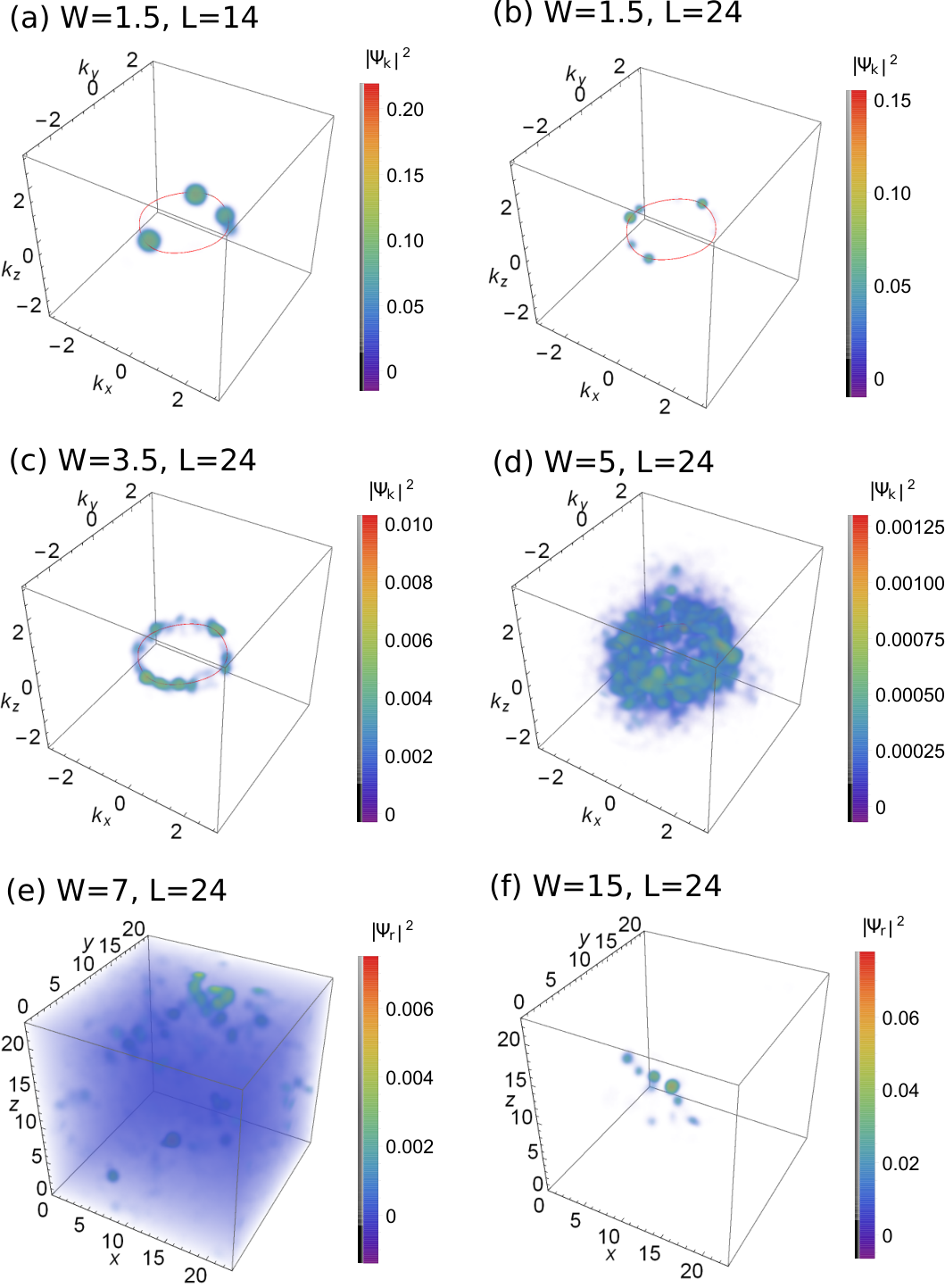
In Figs. S10(e-f), we show plots of the real-space wave function’s PD in the metallic () and insulating () phases. In the former, we see that it spreads all over real space, while in the latter it starts localizing at specific points in space.
S7 Resolution issues
To study the wave function’s PD in momentum space, we focused on the plane . Once the nodal loop is located in this plane, there is an important difference between the resolution that can be attained with respect to the direction. In the latter, the resolution is limited by the grid of planes, separated by . However, in the plane , the grid of momentum-space points with different grows with , providing a better resolution.
We start by addressing the resolution problems in the direction. As an illustrative example, we show the results for in Fig S12. To study this direction independently of the and directions, we considered only points with . We know that the width of the wave function probability in the plane for this disorder strength is . Since there are no significant anisotropies in our model, we expect the width in the direction to be similar, meaning that the separation between planes is times larger than the width of the distribution we want to probe (for any system size!). The consequence is that the distribution assumes a near-plateau for and has a sudden drop after this plateau [Fig S12(a)]. These problems persist to larger , although they become less significant [Fig S12(b)].
We now turn to the small disorder resolution problems in the plane. In this case, although we have better resolution, it is still finite. To see this, we can define the quantity corresponding as the average between consecutive values of for a given system size. We can obtain it simply by: ordering the values obtained for a given twist in ascending order; computing the spacings ; averaging the spacings for a given twist, and finally averaging over twists. The results are shown in Fig. S13(a) for sizes and show that although our ability to resolve the wave function increases with , it is still bounded by the value of . As shown in the main text, in the MF phase, we have and increases with the disorder strength. For small disorder, the attainable system sizes are not enough to provide a small enough resolution to probe the wave function. The effects of the lack of resolution start appearing for (although still small). We show an example for , where they are clear. In Fig. S13(b), we see that and in Fig. S13(c) that , with for . This could suggest erroneously that the wave function spreads over a fractal dimension for low disorder strengths. However, in Fig. S13(c) we also observe a sudden drop in , that can be inspected by raising above for small . If the resolution was small enough, the curve in Fig. S13(c) should increase continuously from () to (). Indeed, this problematic behavior can easily be reproduced by sampling a Lorentzian distribution of width with . The lack of resolution results in an erroneous scaling , with - in the limit that the , we have . This problem also has direct consequences in the multifractal analysis: becomes smaller (larger) for (), as shown in Fig. S13(d), which can again suggest, erroneously, the existence of a MF regime with a fractal dimension .