Charged particle spectra from capture on Al
Abstract
Published data on the emission of charged particles following nuclear muon capture are extremely limited. In addition to its interest as a probe of the nuclear response, these data are important for the design of some current searches for lepton flavor violation. This work presents momentum spectra of protons and deuterons following capture in aluminum. It is the first measurement of a muon capture process performed with a tracking spectrometer. A precision of better than 10% over the momentum range of 100–190 for protons is obtained; for deuterons of 145–250 the precision is better than 20%. The observed partial yield of protons with emission momenta above 80 (kinetic energy 3.4 MeV) is per capture, and for deuterons above 130 (4.5 MeV) it is . Extrapolating to total yields gives per capture for protons and for deuterons, which are the most precise measurements of these quantities to date.
I Introduction
When a negative muon loses energy by ionization and scattering in matter it encounters the field of the nucleus and at kinetic energies below the order of 10–100 eV it can undergo atomic muon capture Haff and Tombrello 1974; Vogel et al. 1975 forming a bound muon-nucleus state, a muonic atom. The in the muonic atom will typically reach the lowest 1S energy level. The weak interaction of the bound muon with the nucleus leads to nuclear muon capture competing with muon decay. Here is a final state consisting of a residual nucleus and perhaps one or more protons, neutrons, gammas, etc., Measday 2001. In this paper “muon capture” refers to nuclear muon capture.
Muon capture and neutrino-nucleus interaction are closely related processes. The capture process probes nuclear response in the energy range below , providing a valuable validation of theoretical models of importance to current and future neutrino experiments Nieves et al. 2004; Nieves et al. 2011. Upcoming Mu2e Bartoszek et al. 2014 and COMET Kuno 2013 experiments will stop intense negative muon beams in aluminum to look for charged lepton flavor violation. Most of the muons will undergo the nuclear capture process. Secondaries from the capture will create unwanted detector rates. In particular, protons and deuterons from capture are highly ionising and can deaden the tracker. It is important to understand their rates to optimize the detectors. There is an ongoing joint effort between Mu2e and COMET to study muon capture on aluminum in a dedicated AlCap experiment Litchfield 2015. The present analysis, on the other hand, uses an opportunistic dataset acquired by the TRIUMF Weak Interaction Symmetry Test (TWIST) experiment Rodning et al. 2001; Hillairet et al. 2012. The same data were previously analyzed for the electron spectrum from muon decay in orbit (DIO) Grossheim et al. 2009.
A theoretical model to describe the yield and spectrum of protons from muon capture was developed by Lifshitz and Singer Lifshitz and Singer 1978; Lifshitz and Singer 1980. It considers both pre-equilibrium and compound-nucleus emission from the excited nucleus with only 7% of the yield from the pre-equilibrium phase for muon capture on Al. The agreement between the results of these models and data available at that time was reasonably good. The predicted yield for proton emission (plus any number of neutrons) is 4.0% per capture and the corresponding yield for deuterons is 1.2%. For the highest-energy part of the spectrum, the impulse approximation is inadequate and capture on pairs of nucleons must be included Lifshitz and Singer 1988.
Published data on the emission of charged partices from nuclear muon capture come from several types of experiments. Studies with photographic emulsions Morinaga and Fry 1953; Kotelchuck and Tyler 1968; Vaisenberg et al. 1970 provide information on both the spectrum and the yield of charged particles, but are limited in their choice of the target nucleus. Another spectrum measurement with an active target was done by stopping negative muons in a silicon detector Sobottka and Wills 1968. Measurements with external scintillator calorimeters were done for multiple elemental targets, see Budyashov et al. 1971; Krane et al. 1979 and references therein. However, they were only able to detect a small high energy tail of the charged particle spectrum, with the bulk of the spectrum being below the detector threshold. (Note that the proton spectrum in, for example, Sobottka and Wills 1968 peaks at , and a proton at this energy has a range of only dozens of microns in material.) Another class of experiments measures radioisotope production after irradiating a target with negative muons Wyttenbach et al. 1978; Heusser and Kirsten 1972. Those experiments allow to deduce the total amount of charged particles emitted in the capture process, but do not provide any information on their spectra, and can not differentiate reaction channels that produce the same final state nucleus. (For example emission of and versus emission of a deuteron.) The present work is the first observation of the momentum spectra of charged particles from muon capture in a magnetic spectrometer, and it is subject to different systematic uncertainties than calorimetric energy spectra measurements in earlier experiments and in AlCap.
In the absence of data about most of the spectrum of protons from muon capture on Al, the experimental spectrum of charged particles from muon capture on Si Sobottka and Wills 1968 was parameterized by E.V. Hungerford Hungerford 1999 for the MECO experiment Bachman et al. 1996. MECO did not proceed past the design stage, but the same parameterization was later used by Mu2e and COMET for their studies. From the (sometimes contradictory) literature Hungerford estimated the per capture rate for protons to be 10%, and approximated the spectrum as
| (1) |
for kinetic energy of the proton , and as a pure exponent in kinetic energy with different slopes below and above Hungerford 1999. Although some versions of GEANT4 Agostinelli et al. 2003 include code to generate charged particle emission after muon capture, the “MECO spectrum” frequently has been used as a practical solution for simulations of the energy spectrum of protons from muon capture to compare with data or for design purposes.
II Experimental Setup
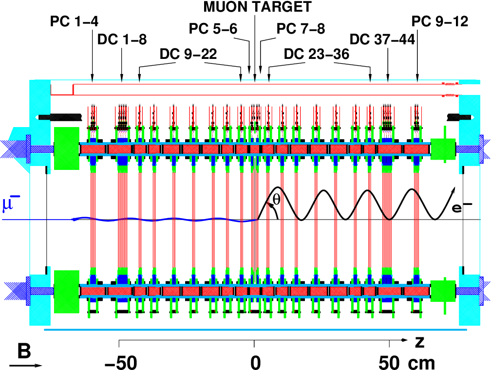
The TWIST detector (Fig. 1) has been described in detail in earlier publications, see Henderson et al. 2005; Bueno et al. 2011. In this section, components that are of particular interest for this analysis will be discussed. The muon beamline was configured to transport a negative beam of approximately with about 1% momentum bite. The incoming beam contained cloud muons (negative muons generated in the proximity of the production target) at a rate of 80 Hz. A thin plastic scintillator at the upstream end of the spectrometer provided a trigger signal, with a threshold chosen to be mostly insensitive to electrons that dominated the beam flux. The trigger was unbiased for muon decay or capture products.
The muons were then transported into the center of the detector and stopped in a thick 99.999% pure Al target. The muon range was adjusted using a gas degrader controlled by a feedback loop. Two stacks of 22 high-precision planar drift-chambers (DCs) were located upstream and downstream of the target. In addition, a total of 8 multi-wire proportional chambers (PCs) were placed at the very upstream and downstream ends of the detector to support the event reconstruction by providing timing information. The target was surrounded by another 4 PCs (PC5,6 upstream and PC7,8 downstream) to enable the measurement of the stopping position of each individual muon. The target itself served as the cathode foil of the two innermost PCs; thus the gas volumes surrounding the target were sensitive. A DC consisted of 80 sense wires at 4 mm pitch surrounded by 6 thick aluminized Mylar cathode foils separated by 4 mm, filled with dimethyl ether at atmospheric pressure. Most DCs were paired into modules of two (so-called u and v modules) with the central foil shared. A relative rotation of the wire planes by 90 degrees allowed for the reconstruction of the position of a hit in the perpendicular plane. The PCs were of similar design, but their wire planes were equipped with wires at 2 mm pitch and a “faster” gas (80:20 mixture of and isobutane at atmospheric pressure) was chosen. Charge collection time in the PCs was faster than 100 ns, while in the DCs it could exceed . In addition to the leading edge time, the time-over-threshold was recorded as an estimate of the size of the signal, approximately proportional to the energy deposit. The gains of PCs 5 and 6 were reduced to avoid saturation of the signal for slow muons; this reduced their detection efficiency for electrons drastically. However, these PCs could then be used to select muons that stopped in the Al target rather than the PC6 gas. The space between the chambers was filled with a (97:3) mixture of helium and nitrogen. The complete detector was contained in a superconducting solenoid magnet, providing a highly uniform field of 2 Tesla.
III Monte Carlo simulation
The Monte Carlo simulation (MC) of the experiment that was developed for previous TWIST measurements was adapted for this analysis. It contains a detailed description of the geometry of the detector and the response of its components to particles traversing the detector Bueno et al. 2011; Hillairet et al. 2012. The MC is implemented in GEANT 3.21 Brun et al. 1993. Its output is in the same format as the detector data and is processed by the same reconstruction program. The simulation was carefully validated by extensive comparisons with data MacDonald et al. 2008; Hillairet et al. 2012. The accuracy of the geometric description and the amount of material in the detector are of particular importance to the current analysis. Earlier TWIST studies did not cover the passage of protons and heavier particles emitted in the muon capture process through detector material. We use “out of the box” GEANT 3.21 description of such processes for this analysis, and assess a resulting systematic uncertainty based on agreement with our data, as described in Sec. V.4.
The simulation starts with a muon entering the detector. (Beam electrons and pile-up muons are also simulated with appropriate rates.) The muon is tracked through the detector with all its GEANT 3 interactions enabled. Typically it ranges out and stops in detector material, at which point a custom routine is called to produce a capture proton, deuteron, etc., or a decay in orbit electron. The daughter particle is subsequently tracked through the detector with all its interactions enabled.
The muon beam momentum and momentum bite affect the muon stopping distribution inside the target. That distribution is expected to have a significant effect on the spectra of capture protons and deuterons exiting the target, because the foil is thick compared to the range of a few-MeV proton in aluminum. A procedure based on matching MC distribution of last wire plane hit by the incoming muon to data Hillairet et al. 2012 was used to tune beam parameters in the simulation. The GEANT3 code does not include the physics of the muon atomic cascade, which affects the last hit plane distribution due to electromagnetic secondaries escaping the target. A GEANT4 version 10.2 MC Allison et al. 2016; Allison et al. 2006; Agostinelli et al. 2003 was used to estimate the effect and derive the corrections of keV/c to MC beam momentum and keV/c to the momentum bite width. Applying the correction shifted the mean muon stopping position by m, and the final uncertainty on the matching between data and MC is Hillairet et al. 2012. The muon stopping distribution is further discussed in Secs. IV.1 and V.
Simulated samples of protons and deuterons from muon capture are only used in this analysis to obtain the detector response function (defined in Sec. IV.5). Therefore, a particular distribution of simulated protons or deuterons in momentum is not important as long as it covers a sufficient kinematic range. An exponential distribution in kinetic energy was used for both types of particles. The analysis also uses samples of electrons from muon decay in orbit (DIO), and triton and alpha particles from muon capture. The shape of the DIO distribution is taken from Grossheim et al. 2009, and shapes of triton and alpha distributions are extracted from a GEANT4 version 10.2p03 simulation of muon capture on aluminum that used the GEANT4 precompound model Quesada et al. 2011. Technically the default constructed muMinusCaptureAtRest process for the negative muon is replaced in our simulations with a new G4MuonMinusCapture instance that is given a G4MuMinusCapturePrecompound argument. The precompound model is expected to be more accurate (Wright and Kelsey 2015, Sec. 4.1) than the Bertini model used in that GEANT4 version by default.
IV Analysis
The objective of the analysis is to determine detector-independent normalized spectra for protons and deuterons from muon capture. The approach is to select a sample of events where a trigger muon stopped in the target and produced a delayed track, and reconstruct these tracks. Positive tracks are protons and heavier particles emitted after muon nuclear capture, and are the main subject of this analysis. Reconstructed distributions of positive tracks from data are corrected for detector efficiency and resolution effects, which are extracted from MC, as described in Sec. IV.5. Negative tracks are due to DIO electrons, and are used to determine the absolute normalization of the result, Sec. IV.4.
The same event selection and reconstruction is applied to real detector data and MC. A single exception in treating data and MC in the same way is not using a cross talk removal algorithm on MC events, because electronic cross talk was not simulated. This is further discussed in Sec. V.
IV.1 Event selection
The data set considered for this analysis contains 57M triggered events. After removal of most crosstalk hits, the hits are grouped by time. The prompt time window included hits belonging to the incident muon. A separate window starting at 400 ns included hits corresponding to muon decay or capture products. The start of the delayed time window was a compromise between the time required to collect all ionization from the DC cells (up to 1000 ns) and the effective muon lifetime in Al (864 ns Grossheim et al. 2009). Requiring wire plane hits up to the stopping target and no hits downstream of the target in the time window corresponding to the trigger time, and demanding the radial position of the stopped muon to be within 2.5 cm of the detector center, yields 22M events. Most of those event are due to muons stopping in the target, but that signature is also consistent with stops in gas or wires of PC6, and such stops comprise about 9% the sample at this selection stage. Out of target stops are suppressed by a cut that uses hit time-over-threshold measurements in PC5 and PC6 as proxy for muon energy deposition Bueno et al. 2011; Bueno 2010. The cut suppresses out of target stops to below 0.5%, which is negligible for the present analysis. It also carves the muon stopping distribution inside the target as shown by the MC simulation in Fig. 2. (The quasiperiodic bump structure in the figure, as well as in Figs. 6 and 7 below, is an artifact caused by an interplay of 3 different discretizations: single precision floating point numbers in GEANT 3, packing of real numbers into integers in TWIST data format, and the bin size of the final histogram.) The number of events passing the cut is 18M.

Further selection identifies events with charged particles from muon capture or decay. For this analysis, only the downstream chambers were used for measuring decay or capture tracks to avoid complications from the reduced gain of PCs 5 and 6. Also, hits from downstream decay or capture tracks are not affected by leftover gas ionization from the incoming muon. A delayed hit is required in one of downstream PCs 7–12, and beam pile-up as identified by PC1–PC4 is vetoed in the delayed time window. Then timing cuts on the delayed time window with respect to the trigger particle and possible pile-up particles are applied. This selection leaves 2.4M “downstream candidate” events. The efficiency of cuts up to this point is the same for DIO and reconstructable capture tracks, which reduces systematic uncertainty on the normalization.
IV.2 Reconstruction of positively charged tracks from muon capture
Sophisticated track finding and fitting software had been developed to reconstruct muon decay tracks in the TWIST detector Hillairet et al. 2012. It was modified for this analysis to optimize its performance for proton tracks from muon nuclear capture. Protons have higher momentum than Michel positrons, and some are not radially contained in the detector. This leads to many tracks having fewer hits for track finding compared to the positron case. Low energy protons range out in the detector material, and also have only a few hits. These effects motivated the inclusion of PC hit information in the track finding code for the present analysis.
For the original TWIST analysis the positron trajectories were first fit to the wire centers of the hits, and then the track was refined using drift times. Because our drift time correction was only valid for relativistic particles, we chose to use only the wire center fits, as this gave adequate resolution. Energy loss and multiple scattering in the detector materials are incorporated in TWIST fits Hillairet et al. 2012. For this work the values were changed to ones appropriate for protons.
Fiducial cuts are made to include only tracks that can be reconstructed reliably with adequate resolution. Thus tracks must have , , and . Here is the angle between the detector axis pointing downstream and the initial momentum direction of the particle. The transverse distance between the position of the stopped muon and the extrapolation of the track to the target plane is required to be less than cm. The number of events with positive tracks passing all the cuts is 22.3k.
The RMS momentum resolution of reconstructed proton tracks is better than 8% between 100 and 200. For deuterons it is better than 15% between 150 and 300. The product of reconstruction efficiency and acceptance for protons and deuterons based on MC is shown in solid lines in Fig. 3.


IV.3 Separation of protons and deuterons
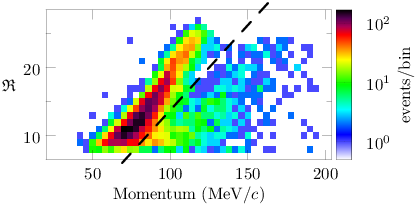
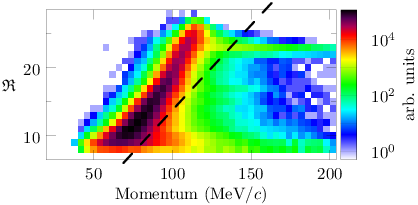
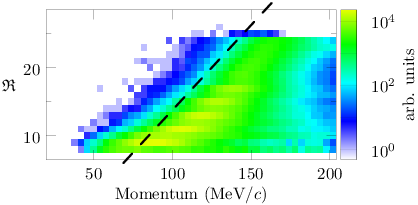
The probability of events being protons or deuterons is based on the difference of range in material vs momentum relationship between protons and deuterons. A subset of events where the track ranges out in the detector material (contained sample) is identified by requiring that the helical extrapolation of the track starting at the target does not exit the instrumented part of the detector radially, and that the range of DC planes hit by the particle ends at or before the last downstream DC. The cut was based on just DC chambers because of a higher noise level observed in the outer PCs. The range of planes hit by the particle was defined to start at the stopping target and include all planes with hits on the fitted track, as well as adjacent downstream planes with contiguous hits in the track time window. The adjacent planes were included to account for the fact that our tracking drops hits at the end of particle range, because in that region the trajectory is dominated by random scattering and the hits do not contribute information about the track initial kinematic. In the TWIST planar detector geometry the amount of material traversed by a particle that crosses a detector layer is proportional to . Therefore the number of planes (DCs and target PCs) traversed by a track was divided by and used as the track range variable . A distribution of track range vs momentum in data is shown in Fig. 4a. MC generated plots for protons and deuterons separately are shown in Figs. 4b and 4c.
Tracks that are not contained provide information about the momentum distribution of events and are combined with the contained sample in the likelihood function used in the analysis, as described in Sec. IV.5.
IV.4 DIO Normalization
Both the electron spectrum and TWIST detector response to it are known with high precision Grossheim et al. 2009, which allows to use reconstructed negative tracks to determine the number of muon decays in the selected sample of events. The ratio of muon capture events to DIO in Al has been measured to be 0.609:0.391, with an uncertainty of 0.001 Suzuki et al. 1987, therefore a per-capture normalization for the positive track sample can be determined from reconstructed negative tracks.
Only downstream muon decays are counted in this analysis. This provides almost 0.7M DIO events for the normalization sample, rendering the statistical uncertainty negligible. The sample is known to be unpolarized Grossheim et al. 2009.
The advantage of using DIO tracks for normalization is that efficiencies of cuts that deal with muon pre-selection or pile-up particles are identical for muon capture and decay events, providing data-to-data and MC-to-MC cancellations in the normalization, without requiring to match absolute cut efficiencies in data and MC.
IV.5 Unfolding
The extraction of the desired physics result, “truth level” momentum spectra (), from experimentally measured quantities that are smeared by the detector resolution is called unfolding. In this study the data observables are the bin contents in the exclusive channels (contained and uncontained), where reconstructed bin index runs over all bins in the range vs momentum “contained” and momentum spectrum “uncontained” histograms. The detector response is the expectation value of the number of reconstructed events in bin for a single proton (or deuteron) emitted in the nuclear capture in the target with true momentum . It describes all the detector effects: acceptance, efficiency, and resolution—but is independent of the physics spectra that are being measured. In practice the detector response is approximated by a matrix obtained by binning the true momentum variable axis: . The response matrix can be determined from Monte-Carlo simulation. If the bin size for the true momentum variable is much smaller than the momentum resolution, the result does not depend on a particular momentum spectrum used in the simulation—the only requirement is that the simulation reaches sufficient statistics in all of the phase space important for the measurement. This study used true momentum bin size.
The expected values of the data observables can be written as
| (2) |
where represent the background. Because many bins in the data sample contain only a few entries, the Poisson statistics must be taken into account. A maximum likelihood estimator for could be formed by maximizing
| (3) |
for the measured set of . However the unfolding problem is known to be ill-posed: truth level spectra that are significantly different from each other can map into detector distributions that have only infinitesimally small differences Blobel 1984; Cowan 1998; Cowan 2002; Prosper and Lyons 2011. The best possible unbiased solution of an unfolding problem would have an unacceptably large variance even if that solution saturated the minimal variance bound Cowan 1998. It has been shown that approximate solutions to unfolding problems can be obtained by using a regularization procedure Tikhonov 1963a; Tikhonov 1963b; Phillips 1962, which reduces the variance of the result at the price of introducing a bias. Regularized unfolding can be performed by maximizing a combination of the log likelihood of data and a regularization functional
| (4) |
where is the regularization parameter. A widely used Tikhonov regularization imposes a “smoothness” requirement on the spectrum by penalizing the second derivative of the solution:
| (5) |
It therefore biases the result towards a linear function. Another well established regularization, the maximum entropy (or “MaxEnt”) approach Cowan 1998, is based on the entropy of a probability distribution Shannon 1948:
| (6) |
It biases the result towards a constant. A useful feature of the MaxEnt approach is that it guarantees that the result will be positive everywhere, as is required for particle emission spectra.
Our initial attempts using a maximum likelihood fit to data with standard regularization procedures consistently produced unphysical rising behavior of the result at the high momentum end of the unfolding range, no matter where the end of the range was defined. There were two factors that caused this: one was the contribution of the overflow region, i.e. the part of the spectrum above the unfolding cutoff. While the spectrum is falling at high momenta, its value just above a cutoff is similar to the value just below, leading to the last few bins in the unfolding range having similar contribution to the reconstructed spectrum to the first few bins above the range. The second factor was the bias from the unfolding regularization term. The high momentum region has small data statistics, and is therefore more susceptible to the bias. This effect can be mitigated by choosing a regularization term that biases towards the “correct” physics distribution. The functions are sharply falling—the spectra are known to be exponential in kinetic energy for large energies. The Tikhonov regularization term biases towards a straight line, and MaxEnt towards a constant; none of these is a good model for the high energy tail of the distribution. A cross-entropy regularization term Cowan 1998 can be used to bias towards a fixed “reference distribution”, but in our case the exponential slopes are unknown parameters that we want to measure.
We addressed both of those issues by utilizing a novel unfolding method Gaponenko 2019. In this approach are arbitrary functions below an unfolding cutoff, and physically motivated exponentials in kinetic energy above the cutoff, with parameters of the exponents included in the fit. The continuation of the solution with a parametrized function outside of the unfolding region provides a correct handling of the overflow region contribution. Another key idea is to impose regularization not on the complete physics spectrum, but on just the “arbitrary function” part of it, with the overall exponential behavior factored out. Then a regularization term that biases its spectrum to a constant will bias the final physics spectrum towards the desired exponential shape. Specifically, we represent
| (7) |
where and determine the limit of the unfolding region for particle type , is the mass of the particle and its kinetic energy, and are parameters pertaining to the exponential behavior of the spectrum, and is an arbitrary function to be determined from the unfolding. The regularization term has the form (5) or (6) but now acts on instead of :
| (8) |
| (9) |
We used the MaxEnt term to extract the central value and most systematic uncertainties, and Tikhonov term to evaluate the uncertainty related to the regularization itself.
The functions are approximated by linear combinations of cubic basis splines (B-splines) Boor 1978 on their unfolding intervals
| (10) |
Here are the spline coefficients determined from the unfolding process. We require that the resulting spectrum has a continuous second derivative, or , which is provided by having a single-fold spline knot at the endpoint . There are no continuity constraints at , therefore a 4-fold knot is used at that point to support the most general cubic spline shape.
The values and are set by the turn-on of the respective acceptance times efficiency curves, see Fig. 3. The transition point between unfolding and exponential fit regions and , as well as the number and position of intermediate knots, were optimized based on unfolding of multiple, statistically independent mixed samples of simulated protons, deuterons, and the backgrounds described below. The mixed samples were designed to have statistics similar to the statistics of the actual data sample. The Appendix provides more information.
The unfolding accounted for two sources of background in Eq. (2): contribution of heavier than deuteron particles emitted in muon capture (tritons and alphas), and DIO electrons misreconstructed as positive tracks. The shape of each of the two backgrounds was taken from the simulation described in Sec. III, while its normalization was a free fit parameter :
The regularization strength in Eq. (4) should be chosen to provide an optimal balance between the variance and the bias of the result. The method used in this study was inspired by the L-curve approach Hansen 1992; Hansen and O’Leary 1993, and is the following. For a given the maximization of yields particular values of and . We consider a parametric curve , and use the corresponding to the point of the maximum curvature of that curve as the optimal solution. This choice of L-curve variables for the log-likelihood fit and Tikhonov regularization corresponds to the classical L-curve defined for a unfolding Hansen 1992. For the MaxEnt regularization we explored several functions of and chose based on the tests with Monte-Carlo samples.
Both data and simulation sample sizes contribute to the statistical uncertainty of the result. To estimate the data contribution, the central values of , , and the backgrounds were determined first by performing unfolding on the actual data sample. Those values were used to calculate expectation values for each data bin using Eq. (2). Then “pseudodata” contained and uncontained histograms were produced by sampling an appropriate Poisson distribution for each bin, and the whole unfolding procedure, including a new choice of the optimal , was performed on that pseudodata sample. The procedure was repeated for 25 statistically independent pseudodata samples, and the variance of was computed from pseudodata unfolding results. The contribution of simulation statistics was estimated by splitting a simulation sample into parts and performing unfolding on real data using only one part of that MC sample at a time, and looking at the variation of the result. The sizes of MC samples were confirmed to be sufficiently large, so that the statistical uncertainty of the result is dominated by the real data statistics.

The momentum spectrum of reconstructed data tracks is shown in Fig. 5. Panels (a)–(e) show the spectrum of the contained tracks in slices of the track range variable (defined in Sec. IV.3). The panel (f) shows the spectrum of uncontained tracks. The fitted values of are also shown in these plots. Fit component yields are 19.1k protons, 2.9k deuterons, 250 heavier than deuteron particles, and 12 misreconstructed DIO events for the 22.3k sample of data tracks. The fit agreement with data is excellent for the uncontained spectrum, and is good for most bins of the contained spectrum. There is a discrepancy for longer range tracks, clearly visible in Fig. 5(e). The peak in the reconstructed MC track momentum distribution is shifted down compared to the data peak by about 3%. This is further discussed in Sec. V.4.
Section VI below shows unfolded , and the Appendix provides more technical details on the fit results.
V Systematic uncertainties
A discrepancy between the simulation of an effect and its actual impact on data would introduce a systematic error in the result. Systematic uncertainties are estimates of the size of such errors. In this study they are typically evaluated by modifying a parameter in simulation and measuring the effect on the resulting yields and spectra by performing the complete unfolding procedure with the modified sample. Another source of systematic error is the unfolding bias. It is estimated by performing unfolding of data with baseline MC samples while modifying some of the settings in the procedure. The rest of this section provides details on individual uncertainties, and Table 1 gives a summary of their effects on the measured yield of protons and deuterons. Figures 10, 11 in the Results section show the momentum dependent total uncertainty of the unfolded spectra, which includes a quadratic sum of all the systematic uncertainties discussed in Secs. V.1–V.6 below.
Among systematic uncertainties the most important ones for proton are cross talk (below 200) and method bias (above 200). For deuteron, the energy loss systematic dominates in most of the momentum range below 300, and cross talk and heavy particle background uncertainties become dominant above 300.
V.1 Muon stopping position
The muon beam momentum in the baseline simulation was tuned as described in Sec. III, resulting in a uncertainty on the stopped muon position. Modified simulation samples were produced by changing the beam momentum by . The resulting shifts in the stopped muon distribution are shown in Fig. 6. The momentum modification shifted the peak position by about 10 times the uncertainty. The stopping position systematic uncertainty was evaluated by taking the difference between data unfolding results with the sample and sample, and scaling it down by a factor of 20. Although the simulation samples were produced by modifying the beam momentum, this systematic uncertainty also covers other effects that shift the stopping distribution, such as differences in the amount of material in the muon path between data and MC and simulation of muon .
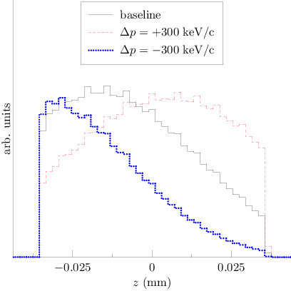
V.2 Carving of the muon stopping distribution by the PC5,6 cut
The PC5,6 cut that suppresses out of target stops changes the shape of the muon stopping distribution for the accepted event sample, see Fig. 2 in Sec. IV.1. The effect of the cut depends on the resolution of the cut variable, which is the time over threshold measurement in the wire chambers. A comparison of time over threshold spectra for data and MC showed that simulated distributions were sharper than data. To evaluate the corresponding systematic effect, time over threshold values were smeared in simulated samples to make MC shapes match those in data, and full analysis chain re-done with the smearing applied. The effect of the smearing on the muon stopping distribution is shown in Fig. 7. We treat the difference between unfolding results for the baseline and smeared analyses as the systematic uncertainty corresponding to the chamber hit time over threshold modeling.

V.3 Crosstalk
Electronic crosstalk was a minor effect for minimum ionizing positron tracks from muon decay Hillairet et al. 2012, and was not implemented in the simulation. Instead, an algorithm to flag crosstalk hits in data was developed. The algorithm uses the fact that crosstalk hits are delayed with respect to the real hit that induced them, and have smaller time over threshold values than most real hits. Hits flagged as crosstalk were ignored by track reconstruction.
Crosstalk is more important for heavily ionizing proton and deuteron tracks. To evaluate its effect in the present analysis, data reconstruction and unfolding were re-done after “un-flagging” at random a fraction of identified crosstalk hits. An increased amount of crosstalk at tracking input reduces the number of reconstructed tracks and changes the unfolded spectrum. This effect is linear in the “un-flagging” fraction range from 0 to at least 0.1. Therefore the difference between the unfolding result for an “un-flagging” setting that doubles the amount of residual crosstalk hits and the baseline result provides an estimate of the systematic uncertainty caused by imperfect crosstalk removal.
To determine the correct “un-flagging” setting to measure the systematic, a sample of data events with positive tracks having was analyzed for different configurations of hit wires in a DC plane. A single wire hit is attributed to a real signal from the track. Two adjacent wires may be due to two real or one real and one “extra” hit. A track with less than a angle can not cause ionization in more than 2 square gas cells, therefore if more than 3 wires are hit there are “extra” hits in the plane. Also any configuration with non-adjacent hit wires must have “extra” hits. Some of the “extra” hits are crosstalk, while others are produced by extra particles in the event (such as a delta electron from the proton track). An extra particle can produce hits in multiple planes, while crosstalk hits in different planes are not correlated. This allows to disentangle the two effects. Figure 8 shows observed rates of correlated and uncorrelated hits in DC22,23. As is expected, the rate of correlated hits does not change with the “un-flagging” fraction setting, while the rate of uncorrelated hits grows linearly, confirming their crosstalk origin. The baseline rate of uncorrelated extra hits doubles for the the “un-flagging” fraction of 0.05, therefore this setting was used to determine the crosstalk systematic uncertainty.

V.4 Charged particle energy loss in detector material
This analysis relies on the modeling of proton and deuteron energy loss in material by out-of-the-box GEANT 3.21 Brun et al. 1993. The discussion in section PHYS430 of the GEANT manual suggests that the model is accurate to a few percent for low energy protons. Reconstructed momentum spectra of contained tracks in our setup provide an experimental handle on the quality of the energy loss model. There is a visible discrepancy between data and simulation in the position of the momentum distribution peak for protons ranging out deep in the detector, see Fig. 5(e). The most probable momentum in data is 92.4 while in MC it is 88.7. The about 4% difference is consistent with the expected accuracy of the simulation.
To evaluate the impact of the discrepancy on the final result, various changes to the simulation code have been tried. The original GEANT3 computed energy loss for protons was scaled by velocity dependent factors. In other simulation runs the amount of material in various parts of the detector was varied. While some of the variations improved data-MC agreement for contained tracks with long range, most of them broke the agreement for shorter contained or uncontained tracks. The variation that showed the best improvement for long contained tracks without introducing discrepancies in other regions was a 20% increase in the density of the drift chamber DME gas. Because the increased gas density also affects the muon stopping distribution, the muon beam momentum in the simulation was adjusted to mostly compensate for the change. A small correction compensating for a residual shift of the muon stopping distribution was applied to the difference between unfolding results with the modified simulation and the baseline to obtain the final estimate of the systematic uncertainty.
V.5 Heavy particle background simulation
The data unfolding fit included triton and alpha particles from the nuclear capture as a single background component with fixed shape and floating normalization. The shapes of triton and alpha distributions and their relative yields for the baseline fit were taken from the GEANT4 precompound model as described in Sec. III. The Bertini Cascade as implemented in GEANT4 Wright and Kelsey 2015 provided an alternative model for the heavy particle spectra. The difference between the models is illustrated in Fig. 9. The systematic uncertainty was estimated as the difference between the unfolding results when using baseline and alternative inputs for the heavy particle background.
Protons are well separated from heavier particles by track range and momentum, so the proton yield is only weakly affected by the modeling of triton and alpha emissions, as can be seen in Table 1. The deuteron result, on the other hand, is directly influenced by simulation of this background.

V.6 Method bias
The proton and deuteron spectra are approximated by cubic splines. To estimate the systematic uncertainty resulting from such approximation, the unfolding procedure was re-done by increasing the number of splines in the basis set by one for protons or deuterons, one variation at a time. The variation of the proton parameterization changed the measured partial yield by for protons and for deuterons. The variation of the deuteron parameterization produced a change in the proton result and in the deuteron one.
The regularization term in the unfolding procedure biases the result. To estimate the bias, Tikhonov regularization term was used instead of the default MaxEnt form. This resulted in a change in the proton yield and change in the deuteron yield.
The quadratic sum of the pararameterization and regularization effects is shown in Table 1 in the “Method” line.
V.7 Other effects
Deuteron breakup in detector material is a potential source of systematic uncertainty. A dedicated MC using cross sections from Refs. Auce et al. 1996; Huu-Tai 2006 showed that the fraction of deuterons breaking up in the detector was at the level of , and thus negligible.
The background from DIO electrons misreconstructed as positive charge tracks is included in the fit. It contributes only at lowest momenta and contributes negligible uncertainty to the measured spectra.
The geometry of the detector and the spectrometer magnetic field are known to a high accuracy Henderson et al. 2005; Bueno et al. 2011, making the uncertainy due to momentum scale calibration negligible.
The proton and deuteron spectra are normalized per muon capture as described in Sec. IV.4. The uncertainties due to the knowledge of the DIO spectrum and the data sample size have a negligible effect on the final result.
| Uncertainty | proton | deuteron |
|---|---|---|
| Crosstalk | 0.00205 | 0.00018 |
| Stopping position | 0.00010 | 0.00001 |
| Stopping distribution | 0.00049 | 0.00020 |
| Energy loss | 0.00025 | 0.00032 |
| Background | 0.00004 | 0.00036 |
| Method | 0.00032 | 0.00026 |
| Combined systematic | 0.00215 | 0.00061 |
| Data statistics | 0.00066 | 0.00088 |
| MC statistics | 0.00006 | 0.00009 |
| Total | 0.00225 | 0.00108 |
VI Results
Figures 10 and 11 show the differential yields of protons and deuterons per muon capture and . As described in Sec. IV.5, the unfolding splines are defined in the 80 to 230 range for protons, and 130 to 230 for deuterons. The higher momentum data included in the fit assume exponential (in kinetic energy) behavior, so there is no explicit upper cut off for the fit range. We define an effective upper cut off for this measurement as the momentum beyond which the expected contribution of the exponential tail to the reconstructed spectrum equals one event. This cut off is about 300 for protons and 400 for deuterons. The uncertainty on the proton spectrum below 150 is mostly systematic, while above 150 it is dominated by the data sample statistics. For deuteron the statistical and systematic contributions are of similar size in most of the range.


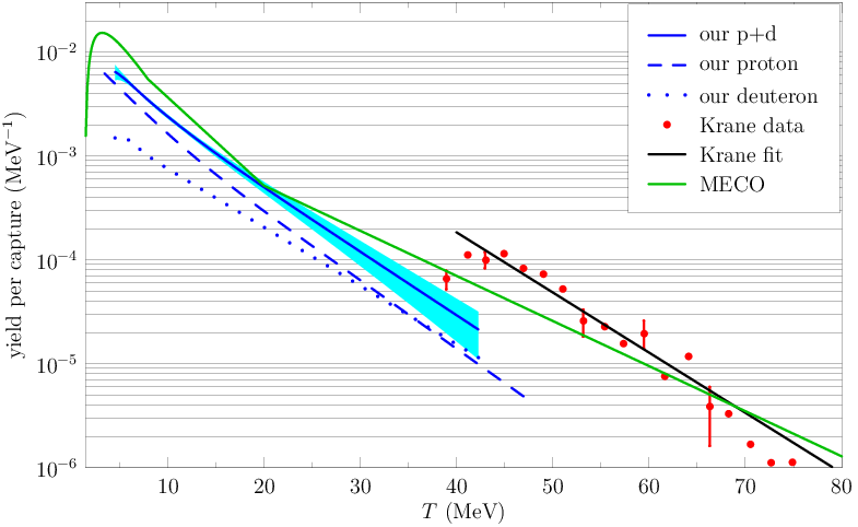
The figures also show the “MECO spectrum” Hungerford 1999 where deuterons are assumed to have the same spectrum shape in kinetic energy as protons, and spectra predicted by GEANT4 version 10.2p03 with the precompound model, as detailed in Sec. III. (The default codes for muon capture are in poor agreement with our data and are not shown.)
Integrating the unfolded spectra while taking into account bin-to-bin correlations, we obtain the per capture yields of
| (11) |
for protons above and
| (12) |
for deuterons above . The correlation coefficient between the visible yields, including all statistical and systematic uncertainties, is .
To extrapolate to the total yield we normalize the GEANT4 precompound or MECO prediction to match our measured spectrum just above the threshold, and add the integrated yield up to our threshold to the measured yield. We take the average between GEANT4 precompound and MECO results as the central value, and include half the difference in the extrapolation uncertainty. Another, smaller, contribution to the extrapolation uncertainty is obtained by varying the matching momentum. The resulting per capture yields are
| (13) |
for protons and
| (14) |
for deuterons. These numbers are close to the corresponding theoretical predictions of and Lifshitz and Singer 1980. Radioisotope yields for muon capture on aluminum are reported in Wyttenbach et al. 1978 and Heusser and Kirsten 1972 as for the final state consistent with emission, and for . Note that the activation measurement technique can not distinguish separate and particles from a deuteron. The sum of the earlier measurements compares well to our sum of extrapolated proton and deuteron yields of .
A measurement of the energy spectrum of charged particles from muon capture on aluminum above is reported in Krane et al. 1979. Figure 12 reproduces data points and the fit from that paper, along with our proton and deuteron results converted to kinetic energy spectra. While the slope of the fit in Krane et al. 1979 agrees with that of our curve, the previously reported yield around is significantly higher. Figure 12 also shows that the MECO spectrum Hungerford 1999 provides, withing the uncertainties, an upper bound on the sum of proton and deuteron emission. Individual proton and deuteron spectra are bound by the MECO curve along with the 65% proton and 35% deuteron emission fractions suggested in Hungerford 1999.
VII Summary
The TWIST data taken with a beam incident on Al have been analysed for positive charged particles from muon capture. The detector was sensitive to protons with momentum above 80 and deuterons above 130. These ranges are found to contain about of the yield for each particle. A precision of better than 10% over the momentum range of 100–190 for protons is obtained; for deuterons of 145–250 the precision is better than 20%. The results are presented in a format suitable for building an event generator for use in simulations. They have immediate application to the design of experiments searching for to conversion. These spectra are of interest as input to an improved theoretical understanding of the physics of muon capture on nuclei. They are strongly selective of the GEANT4 precompound model over the other presented choices. The total per capture yields of for protons and for deuterons are the most precise measurements of these quantities to date.
Acknowledgements.
We thank all TWIST collaborators who contributed to detector construction and data taking, as well as TRIUMF staff. We thank Konstantin Olchanski who promptly fixed any computer problems we had. This work was supported in part by the Natural Sciences and Engineering Research Council of Canada, the Russian Ministry of Science, and the U.S.A. Department of Energy. One of the authors (Andrei Gaponenko) was supported by the resources of the Fermi National Accelerator Laboratory (Fermilab), a U.S. Department of Energy, Office of Science, HEP User Facility. Fermilab is managed by Fermi Research Alliance, LLC (FRA), acting under Contract No. DE-AC02-07CH11359.*
Appendix A Parameterization of the unfolded spectra
The notation used in the Appendix is defined in Sec. IV.5. The parameterization of the measured spectra is given by Eq. (7), with the arbitrary functions approximated by linear combinations of cubic B-splines Boor 1978 per Eq. (10). The splines for the proton spectrum are defined by the sequence of knots , resulting in a set of two basis functions that are illustrated in Fig. 13. The deuteron spline sequence is , similarly resulting in two cubic splines. The parameters of the unfolded proton and deuteron spectra are shown in Table 2, and their correlations in Table 3. The uncertainties shown in Table 2 include statistical and most systematic contributions. The parameterization shape uncertainty is not representable in terms of the fixed set of fit parameters, and is the only contribution that is not included.

| Parameter | Value | Uncertainty |
|---|---|---|
| () | ||
| () | ||
| () | ||
| () | ||
| 1.00 | 0.96 | -0.48 | -0.84 | -0.14 | -0.26 | -0.03 | -0.21 | |
| 1.00 | -0.64 | -0.76 | -0.26 | -0.39 | -0.05 | -0.24 | ||
| 1.00 | 0.06 | 0.48 | 0.63 | 0.28 | 0.34 | |||
| 1.00 | 0.09 | 0.07 | -0.15 | -0.10 | ||||
| 1.00 | 0.90 | 0.23 | -0.36 | |||||
| 1.00 | 0.32 | -0.01 | ||||||
| 1.00 | -0.04 | |||||||
| 1.00 |
References
- Haff and Tombrello (1974) P. Haff and T. Tombrello, Negative muon capture in very light atoms, Ann. Phys. 86, 178 (1974).
- Vogel et al. (1975) P. Vogel et al., Muon capture in atoms, crystals and molecules, Nucl. Phys. A254, 445 (1975).
- Measday (2001) D. Measday, The nuclear physics of muon capture, Phys.Rept. 354, 243 (2001).
- Nieves et al. (2004) J. Nieves, J. E. Amaro, and M. Valverde, Inclusive quasi-elastic neutrino reactions, Phys. Rev. C70, 055503 (2004), [Erratum: Phys. Rev.C72,019902(2005)].
- Nieves et al. (2011) J. Nieves, I. Ruiz Simo, and M. J. Vicente Vacas, Inclusive Charged–Current Neutrino–Nucleus Reactions, Phys. Rev. C83, 045501 (2011).
- Bartoszek et al. (2014) L. Bartoszek et al. (Mu2e), Mu2e Technical Design Report (2014), arXiv:1501.05241 [physics.ins-det] .
- Kuno (2013) Y. Kuno (COMET), A search for muon-to-electron conversion at J-PARC: The COMET experiment, PTEP 2013, 022C01 (2013).
- Litchfield (2015) R. P. Litchfield (AlCap), Status of the AlCap experiment, Proceedings, 16th International Workshop on Neutrino Factories and Future Neutrino Beam Facilities (NUFACT 2014): Glasgow, Scotland, UK, 25–30 August 2014, PoS NUFACT2014, 095 (2015).
- Rodning et al. (2001) N. L. Rodning et al. (TWIST), TWIST - The TRIUMF Weak Interaction Symmetry Test: The Michel parameters from mu+ decay, Tau lepton physics. Proceedings, 6th International Workshop, TAU 2000, Victoria, Canada, September 18-21, 2000, Nucl. Phys. Proc. Suppl. 98, 247 (2001).
- Hillairet et al. (2012) A. Hillairet et al. (TWIST Collaboration), Precision muon decay measurements and improved constraints on the weak interaction, Phys.Rev. D85, 092013 (2012).
- Grossheim et al. (2009) A. Grossheim et al. (TWIST Collaboration), Decay of negative muons bound in Al-27, Phys.Rev. D80, 052012 (2009).
- Lifshitz and Singer (1978) M. Lifshitz and P. Singer, Charged particle emission following muon capture in complex nuclei, Phys. Rev. Lett 41, 18 (1978).
- Lifshitz and Singer (1980) M. Lifshitz and P. Singer, Nuclear excitation function and particle emission from complex nuclei following mu capture, Phys. Rev. C 22, 2135 (1980).
- Lifshitz and Singer (1988) M. Lifshitz and P. Singer, Meson exchange currents and energetic particle emission from capture, Nucl. Phys. A476, 684 (1988).
- Morinaga and Fry (1953) H. Morinaga and W. Fry, Nuclear capture of negative mesons in photographic emulstions, Nuovo Cimento Ser. 9 10, 308 (1953).
- Kotelchuck and Tyler (1968) D. Kotelchuck and J. V. Tyler, Search for a conserved-vector-current mechanism in the emission of protons from stars in emulsion, Phys.Rev. 165, 1190 (1968).
- Vaisenberg et al. (1970) A. O. Vaisenberg, E. D. Kolganova, and N. V. Rabin, High energy protons due to absorption of muons by emulsion nuclei, Yad. Fiz. 11, 830 (1970).
- Sobottka and Wills (1968) S. E. Sobottka and E. L. Wills, Energy spectrum of charged particles emitted following muon capture in , Phys. Rev. Lett. 20, 596 (1968).
- Budyashov et al. (1971) Yu. G. Budyashov, V. G. Zinov, A. D. Konin, A. I. Mukhin, and A. M. Chatrchian, Charged particles from the capture of negative muons by the nuclei , , and , Sov. Phys. JETP 33, 11 (1971), [Zh. Eksp. Teor. Fiz.60,19(1971)].
- Krane et al. (1979) K. Krane, T. Sharma, L. Swenson, D. Mcdaniels, P. Varghese, et al., Energetic charged particle spectrum following capture by nuclei, Phys.Rev. C20, 1873 (1979).
- Wyttenbach et al. (1978) A. Wyttenbach, P. Baertschi, S. Bajo, J. Hadermann, K. Junker, et al., Probabilities of muon induced nuclear reactions involving charged particle emission, Nucl.Phys. A294, 278 (1978).
- Heusser and Kirsten (1972) G. Heusser and T. Kirsten, Radioisotope production rates by muon capture, Nucl.Phys. A195, 369 (1972).
- Hungerford (1999) E. V. Hungerford, Comment on proton emission after muon capture, MECO Note 34 (1999), available as arXiv:1803.08403.
- Bachman et al. (1996) M. Bachman et al., A Search for with Sensitivity Below (1996), AGS Letter of Intent.
- Agostinelli et al. (2003) S. Agostinelli et al. (GEANT4), GEANT4: A Simulation toolkit, Nucl. Instrum. Meth. A506, 250 (2003).
- Henderson et al. (2005) R. S. Henderson et al., Precision planar drift chambers and cradle for the TWIST muon decay spectrometer, Nucl. Instrum. Meth. A548, 306 (2005).
- Bueno et al. (2011) J. Bueno et al., Precise measurement of parity violation in polarized muon decay, Phys. Rev. D 84, 032005 (2011).
- Brun et al. (1993) R. Brun, F. Bruyant, F. Carminati, S. Giani, M. Maire, A. McPherson, G. Patrick, and L. Urban, GEANT: Detector Description and Simulation Tool; Oct 1994, CERN Program Library (CERN, Geneva, 1993) Long writeup W5013, DOI http://dx.doi.org/10.17181/CERN.MUHF.DMJ1.
- MacDonald et al. (2008) R. P. MacDonald et al. (TWIST), A Precision Measurement of the Muon Decay Parameters rho and delta, Phys. Rev. D78, 032010 (2008).
- Allison et al. (2016) J. Allison et al., Recent developments in Geant4, Nucl. Instrum. Meth. A835, 186 (2016).
- Allison et al. (2006) J. Allison et al., Geant4 developments and applications, IEEE Trans. Nucl. Sci. 53, 270 (2006).
- Quesada et al. (2011) J. M. Quesada et al., Recent developments in pre-equilibrium and de-excitation models in GEANT4, Progress in Nuclear Science and Technology , 936 (2011).
- Wright and Kelsey (2015) D. H. Wright and M. H. Kelsey, The Geant4 Bertini Cascade, Nucl. Instrum. Meth. A804, 175 (2015).
- Bueno (2010) J. Bueno, A direct measurement of from muon decay, Ph.D. thesis, The University of British Columbia (Vancouver) (2010), http://dx.doi.org/2429/23724.
- Suzuki et al. (1987) T. Suzuki et al., Total nuclear capture rates for negative muons, Phys. Rev. C 35, 2212 (1987).
- Blobel (1984) V. Blobel, Unfolding Methods in High-energy Physics Experiments, in Proceedings, CERN School of Computing: Aiguablava, Spain, September 9-22 1984 (1984).
- Cowan (1998) G. Cowan, Statistical Data Analysis (Clarendon Press, Oxford, New York, 1998).
- Cowan (2002) G. Cowan, A survey of unfolding methods for particle physics, Advanced Statistical Techniques in Particle Physics. Proceedings, Conference, Durham, UK, March 18-22, 2002, Conf. Proc. C0203181, 248 (2002).
- Prosper and Lyons (2011) H. B. Prosper and L. Lyons, eds., Proceedings, PHYSTAT 2011 Workshop on Statistical Issues Related to Discovery Claims in Search Experiments and Unfolding, CERN,Geneva, Switzerland 17-20 January 2011, CERN (CERN, Geneva, 2011).
- Tikhonov (1963a) A. N. Tikhonov, Solution of incorrectly formulated problems and the regularization method, Soviet Mathematics Dokl. 4, 1035 (1963a), translation of Doklady Akademii Nauk SSSR, 151 (1963) 501–504.
- Tikhonov (1963b) A. N. Tikhonov, Regularization of ill-posed problems, Soviet Mathematics Dokl. 4, 1624 (1963b), translation of Doklady Akademii Nauk SSSR, 153 (1963) 49–52.
- Phillips (1962) D. L. Phillips, A technique for the numerical solution of certain integral equations of the first kind, J. Assoc. Comput. Mach. 9, 84 (1962).
- Shannon (1948) C. E. Shannon, A mathematical theory of communication, Bell Syst. Tech. J. 27, 379 (1948).
- Gaponenko (2019) A. Gaponenko, A practical way to regularize unfolding of sharply varying spectra with low data statistics (2019), arXiv:1906.07918 [physics.data-an] .
- Boor (1978) C. d. Boor, A Practical Guide to Splines (Springer Verlag, New York, 1978).
- Hansen (1992) P. C. Hansen, Analysis of discrete ill-posed problems by means of the L-curve, SIAM Review 34, 561 (1992).
- Hansen and O’Leary (1993) P. C. Hansen and D. F. O’Leary, The use of the L-curve in the regularization of discrete ill-posed problems, SIAM J. Sci. Comput. 14, 1487 (1993).
- Auce et al. (1996) A. Auce et al., Reaction cross sections for 38, 65, and 97 MeV deuterons on targets from to , Phys. Rev. C 53, 2919 (1996).
- Huu-Tai (2006) P. C. Huu-Tai, Systematic study of elastic and reaction cross sections of deuteron induced reactions within the CDCC approach, Nucl. Phys. A 773, 56 (2006).