Evaluation of extremal properties of GARCH(p,q) processes
Abstract
Generalized autoregressive conditionally heteroskedastic (GARCH) processes are widely used for modelling features commonly found in observed financial returns. The extremal properties of these processes are of considerable interest for market risk management. For the simplest GARCH() process, with , all extremal features have been fully characterised. Although the marginal features of extreme values of the process have been theoretically characterised when , much remains to be found about both marginal and dependence structure during extreme excursions. Specifically, a reliable method is required for evaluating the tail index, which regulates the marginal tail behaviour and there is a need for methods and algorithms for determining clustering. In particular, for the latter, the mean number of extreme values in a short-term cluster, i.e., the reciprocal of the extremal index, has only been characterised in special cases which exclude all GARCH() processes that are used in practice. Although recent research has identified the multivariate regular variation property of stationary GARCH() processes, currently there are no reliable methods for numerically evaluating key components of these characterisations. We overcome these issues and are able to generate the forward tail chain of the process to derive the extremal index and a range of other cluster functionals for all GARCH() processes including integrated GARCH processes and processes with unbounded and asymmetric innovations. The new theory and methods we present extend to assessing the strict stationarity and extremal properties for a much broader class of stochastic recurrence equations.
August 11, 2026
Keywords: Cluster of extremes; extremal index; fixed point distributions; GARCH process; multivariate regular variation, particle filtering, stochastic recurrence equations
1 Introduction
Risk management in the stock markets, commonly called market risk management, requires the use of statistical tools and models which aim at reducing the potential size of losses, occurring by sudden drops or growth in the value of stock. Losses can be amplified during periods of large volatility. Risk managers routinely use strategies to handle, model and predict the volatility of daily log-returns, defined as , where , is the price of a generic asset. The behaviour of the extreme values of daily log-returns is critically important for market risk management. Isolated extreme values of daily log-return can often be managed, but there is major risk when there is a clustering of these extreme values, and so the study of this dependence structure during extreme events is essential.
It is standard to assume that the series is a stationary series. The most widely adopted models for are the generalised autoregressive conditionally heteroskedastic (GARCH) models (Bollerslev 1986) and stochastic volatility (SV) models (Taylor 1986). These models are capable of capturing many of the empirical features of daily log-returns. Both processes have heavy tailed marginal distributions with the leading decay rates the same for both models. Where they differ is in terms of their extremal dependence structure. One of the most common ways to measure this is through the lag tail dependence
| (1.1) |
proposed by Ledford and Tawn 2003, with Davis and Mikosch 2009b terming the extremogram. For SV models Breidt and Davis 1998 show that there is no clustering of extreme values, so that for all . Thus extreme values from SV processes occur in temporal isolation. In contrast, for any GARCH() process for at least one value of . But, the values of the extremogram, and other extremal dependence features, are only known for a very restricted subclass of GARCH() processes. The aim of this paper is to derive these extremal features for all GARCH() models used in typical financial applications and to present algorithms for their evaluation.
We consider GARCH() models, for and , of the form
| (1.2) |
where, for every fixed , the random variables and are independent. Furthermore, we assume that are independent and identically distributed continuous random variables with and . The process , commonly referred to as the conditional volatility of , is given by
| (1.3) |
where and the parameters , and , for , have to satisfy additional constraints for the process to be strictly stationary; see Section 2. When , equations (1.2) and (1.3) correspond to an ARCH() process and when
| (1.4) |
they correspond to an integrated GARCH() process, denoted IGARCH(), which is strictly stationary but not second-order stationary. We develop new numerically robust and efficient methods for assessing whether any GARCH() process is strictly stationary. Our results cover all of the GARCH() processes including these special cases.
Existing theoretical and computational methods for deriving extremal properties are well established for special cases of the GARCH() process, namely: for symmetric with , corresponding to the ARCH(1) process (de Haan et al. 1989) and for , corresponding to a GARCH(1,1) (Laurini and Tawn 2012); and for asymmetric with (Ehlert et al. 2015). Additional results of other tails probabilities are derived in the two-dimensional case by Collamore et al. 2014 but are effective only for ARCH(1) as further complications arise for the GARCH().
For general GARCH() models, with arbitrary many theoretical extremal properties have been derived by Basrak et al. 2002, Davis and Mikosch 2009a and Basrak and Segers 2009, including the tails of marginal distributions and some results for the extremal clustering properties. At first sight it seems that these results give everything that is needed for numerical evaluation of the required extremal properties. But this is far from the case, as we will show.
Firstly consider the marginal tail behaviour of and . Basrak et al. 2002 showed that for GARCH() processes there is an explicit theoretical expression for such that for fixed as then
These papers only give an asymptotic limiting expression for the evaluation of , but they do not illustrate its application. We find that direct computation using their expression gives very poor numerical performance. Janssen 2010 presents an alternative approach to evaluate , however that approach applies only under the assumption that the innovation has bounded support, ruling out many important distributions used by practitioners, e.g., being Gaussian or -distributed. Furthermore, the associated numerical methods are very slow. We propose the first reliable and computational efficient numerical algorithms for the valuation of , which are valid irrespective of whether are unbounded or bounded. We also find a new formulation for which gives new insights and we show that for all IGARCH() processes .
Now consider the extremal dependence/clustering features of the process. Basrak and Segers 2009 and Basrak and Segers 2011 propose computational algorithms for their evaluation. However, these methods have major limitations, which they identify, and only apply to some stochastic recurrence equations with bounded innovations, but do not hold for any GARCH() processes, see Section 2.2. So currently no extremal clustering features for GARCH() processes, when , can be evaluated. We propose an entirely new numerical algorithm to evaluate a range of cluster features for any GARCH() process, regardless of the values of and and without imposing any restrictive assumptions.
There are a range of extremal dependence features of GARCH process that are of interest to practitioners. The most standard features are summarised by the time-normalized point process of exceedances of a level , defined by
where tends to the upper endpoint of the distribution of as , such that , for any finite , where and are the marginal distribution and survivor functions of respectively. As , converges to a compound Poisson process , where events occur as in a homogeneous Poisson process with intensity , where is termed the extremal index and with multiplicities distribution denoted by for (Hsing et al. 1988). We use the term clusters to describe the independent extreme events, with the associated multiplicities corresponding to the number/size of extreme values in each cluster. It follows that
| (1.5) |
i.e., the extremal index is the reciprocal of the limiting mean cluster size of extreme values. The smaller the extremal index then the larger the average number of extreme values per cluster. The special case corresponds to there being no clustering of extremes, so extreme values occur in isolation in time. Thus, minimally there is a need to derive and , and to get the latter we need . Other functionals are also of interest to financial institutions for managing the duration of a stress period or predicting the total amount of losses that can be faced in such stress period, such as the aggregate of excesses over a cluster (total loss). These can also be derived using our methods.
All of these cluster functionals can be obtained from the tail chain of the process, which has been widely used for studying extremal clustering (Rootzén 1988, Smith et al. 1997, Segers 2003, Planinić and Soulier 2018). The tail chain is defined for a heavy tailed process in the following way. When , if for any
converges weakly to , with non-degenerate, then the limit process is termed the forward tail chain. For SV models almost surely for all , so large values are not followed by large values for SV processes. In contrast, for any GARCH() process at least one , for , is non-degenerate, and every element of the tail chain is non-degenerate if and , see Section 6.1 for further details.
Similarly, there is a backward tail chain with identical definition for negative . Here is the same value for both forward and backward chains. The connections between forward and backward chains were determined by Janssen and Segers 2014. However, in many cases only the forward chain is required to derive the functionals of interest. For example, the extremogram and the extremal index of can be expressed, respectively, as
In this paper we derive the theory for obtaining the forward tail chain, the extremogram, the extremal index and cluster size distribution for any GARCH() process with bounded or unbounded support for the innovations. We provide a new fast, yet accurate, Monte Carlo algorithm for the numerical evaluation of these extremal features. We first obtain the forward tail chain for the squared GARCH() process and then use this in a filtering argument, similar to de Haan et al. 1989, to derive the features of interest.
The paper is structured in the following way. In Section 2 we give the required background details for the properties of stationary GARCH() processes and the theory of multivariate regular variation that is required for our methodology. In Section 3.1 we give new results for testing stationarity and a new formulation for the tail index . In Sections 3.3 and 4 we derive the tail chain for the series squared and original GARCH() processes respectively, with Section 3.2 containing the key particle filtering algorithm which enables us to sample from a -dimensional extreme state of the tail chain. Critical to the development of this algorithm is the theory of fixed point distributions. Section 5 discusses the novel numerical evaluation of all components of the method, including checking for stationarity and evaluating , and it also illustrates the rapid convergence of the particle filter algorithm. Section 6 has a study of a range of extremal dependence features of the GARCH() process over a variety of parameter values. In Section 7 we identify that the methods and algorithms that are developed here in the context of GARCH() processes immediately extend to a much broader class of stochastic recurrence equations, and so they are likely to have a much wider impact. The proofs of the theorems are given in the Appendix A.
2 Known properties of GARCH() processes
2.1 Strict Stationarity
Let us start by defining strict stationarity for GARCH() processes. We focus on the squared GARCH process, , and rewrite the process as a stochastic recurrence equation (SRE) as this enables the exploitation of a range of established results (Kesten 1973) for such processes, e.g., the existence of results for the marginal distribution.
Let the vector , the matrix and the vector be
| (2.1) |
where , , is the identity matrix of size , is a matrix of zeros with rows and columns and is a column vector of zeros having length . In each case here if then these terms are to be interpreted as being dimensionless. Then it follows that the squared GARCH() processes satisfies the SRE
| (2.2) |
where and are each sequences of independent and identically distributed stochastic matrices and vectors.
The formulation of the SRE via (2.1) is due to Francq and Zakoïan 2010. This SRE formulation is less parsimonious than that of Bougerol and Picard 1992, but has the benefit of covering all GARCH() processes, unlike that of Bougerol and Picard 1992 which does not include the case . In contrast here when we have that the terms in expression (2.1) simplify to
| (2.3) |
where and are scalar and none of the or are included.
For general SRE of the form (2.2), but without the specific specification of and corresponding to a GARCH() process, Francq and Zakoïan 2010 show that it is necessary and sufficient that there is a negative top Lyapunov exponent of for the existence of a unique, strictly stationary solution. Before defining the Lyapunov exponent of a stochastic matrix first consider the spectral radius of a deterministic square matrix , denoted . Here is the greatest modulus of its eigenvalues, and an important algebraic result is , where is any norm on the space of . The extension to a sequence of strictly stationary and ergodic random matrices , for which (here if and 0 otherwise), is such that the top Lyapunov exponent is
| (2.4) |
and is the spectral radius of the sequence . Hence if for all , it is necessary and sufficient that for a strictly stationary process .
So for strict stationarity of the squared and original GARCH() processes and we need for given by expression (2.1) and . The finite moment condition holds for GARCH() processes as , for constants and and so , for a suitable constant and where the last inequality holds as is finite by the model definition (1.2). Consequently we only need to check if .
Unfortunately, expression (2.4) is not an ideal starting point for evaluating . Instead we also have
| (2.5) |
see Francq and Zakoïan 2010. So, via expression (2.5), it would appear a relatively simple simulation can be performed to obtain a reliable Monte Carlo estimate of . However, as we will show in Section 5.2, this is far from the case and a mix of careful asymptotic approximation analysis and numerical evaluation is required to evaluate .
In some special cases we do not need to evaluate to find if the process is strictly stationary, e.g., GARCH() processes are always strictly stationary when ; this includes all IGARCH() processes. It is also known that is necessary but not sufficient for strict stationarity. Therefore, numerical evaluation of is required whenever when .
2.2 Existing Results
Basrak et al. 2002 show that there exists a unique stationary solution to the SRE (2.2) and that this solution exhibits a multivariate regular variation property, i.e., for any , any norm and all ,
| (2.6) |
where denotes vague convergence (Kallemberg 1983), , and is a -dimensional random vector in the unit sphere (with respect to a norm ) defined by , and their elements will be denoted by . If condition (2.6) holds then is said to exhibit multivariate regular variation with index and the distribution of is termed the spectral measure of the vector . See Resnick 1987 for further details on multivariate regular variation. A consequence of the multivariate regular variation property (2.6) for GARCH() processes is that all the marginal variables of have regularly varying tails with index , so in particular for and all
| (2.7) |
So both the squared GARCH() process and its variance have regularly varying tails of index .
It is insightful to consider a slightly rearranged version of limit (2.6) and to be specific about which norm we will use. We take the norm, and define radial, , and angular (two variants and ) random variables by
| (2.8) |
with the dimensional unit simplex. We have two angular variables as the dimensional variable has redundancy in its final dimension as , and so for studying the distribution of angular variables it is simpler to work with the dimensional variable , which is related to by and being without its last component. We use this notation to create a dimensional vector from any dimensional vector on the simplex throughout. Furthermore, for , we use the notation
| (2.9) |
with vector algebra, here and elsewhere, interpreted as being componentwise.
We will denote the limit random variables, that arise in limit (2.6), for by , with the distribution function of , denoted by , defined similarly to distribution (2.9). Subsequently is referred to as the spectral measure, the term coming from multivariate regular variation terminology (Resnick 1987). Then, for , as , the limit (2.6) becomes,
| (2.10) |
From the first expression for the asymptotic form in limit (2.10) we see that the radial variable and the angular variables become asymptotically independent, as the radial variable grows due to , i.e., the variables and are independent. The second term in this limit shows that is a Pareto random variable with tail index , i.e.,
| (2.11) |
There is additional structure imposed on both and by the GARCH() process, which is identified by Basrak and Segers 2009 and Janssen 2010 respectively. We discuss this structure in each case below.
For the GARCH() process, Laurini and Tawn 2012 provided an expression for the spectral measure, for a different description of the angular variable to that used here. For the choice of the angular variable (2.2), for all , their result translates to
| (2.12) |
where is the distribution function of the innovations . When , through highly skilled use of the multivariate regular variation structure, Basrak and Segers 2009 show, that when is independent and identically distributed to , that
| (2.13) |
and uniquely
where the notation where is the indicator of the event . Thus
| (2.14) |
Basrak and Segers 2009 propose an approach to simulate from for an SRE of the form (2.2), with the required distribution being the invariant distribution of a Markov chain and MCMC methods used for its evaluation. However, this method cannot be used for general GARCH() processes for the following reasons. Firstly, they make an assumption that is bounded, which excludes the possibility of being, for example, Gaussian or distributed. Much more critically though, Basrak and Segers 2011 note that the proof that is the stationary distribution of the Markov Chain that they proposed was flawed, and their claimed results only hold under one of two very specific conditions on the matrix in the SRE framework (2.2). Neither of these conditions are satisfied by the form of for GARCH processes, when , even with a bounded . Thus the algorithm proposed by Basrak and Segers 2009 cannot be used for obtaining for a GARCH process. Our approach in Section 3.2 overcomes both of these restrictions.
Next we focus on how is determined. In particular, Basrak et al. 2002 showed that there exist a which is the unique positive solution of the equation
| (2.15) |
where here and throughout the matrix norm we use will use is , where is th element of matrix . For the GARCH() process Mikosch and Stărică 2000 show that is simple to evaluate using expression (2.15). Specifically, taking as in expression (2.3) we have that
from which it simply follows that expression (2.15) holds and satisfies
| (2.16) |
Setting for the GARCH() process gives the same result for derived by de Haan et al. 1989 for the ARCH(1) process. For general GARCH() processes no such existing simplification of equation (2.15) gives an easier expression for . So it is natural to try to find by a numerical solution of the limit equation (2.15). However, direct numerical solution is non-trivial due to numerical instabilities.
The only existing feasible method to evaluate was proposed by Janssen 2010, which exploits Kesten 1973. With specified in (2.2) the conditions required for the results of Kesten 1973 apply and the equality
| (2.17) |
holds for all continuous functions , all unit measures on the space , and where is a constant. The special case of in (2.17) gives the simplification
| (2.18) |
For any given , whatever the chosen unit measure , if the pair satisfies equality (2.17), then is determined solely by , i.e., not by the choice of .
As we know from condition (2.13) that the moment of is equal to , where on the space then it follows from property (2.18) that when . Kesten 1973 and Janssen 2010 shows that there is only one solution to equation (2.13), so is the unique solution of
| (2.19) |
and that the unit measure must correspond to the distribution function . Thus if we can find, or simulate from, we can find . To evaluate all that is required is to define a class of unit measures , over , which contains within it as an interior point , and then vary until property (2.19) is found.
Janssen 2010 proposes an algorithm to simulate from a class of functions which adapts the invalid algorithm of Basrak and Segers 2009. This gives a valid method for finding and but critically it only applies when the innovations have bounded support. Therefore there is a need for an algorithm to cover cases where have unbounded support. In Section 3.2 we describe such an algorithm that applies whatever the support of . Furthermore, our methods for calculating , have substantial computational performance and efficiency gains compared to the algorithm of Janssen 2010; see Section 5.6.
3 Extremal properties of squared GARCH processes
3.1 New formulations for and
Expression (2.5) suggests using Monte Carlo for the evaluation of , by taking to be very large. This approach suffers from serious numerical instabilities. As the norm of the product is tending to zero it seems sensible to first normalise the size of the individual terms in the product. We do this be scaling each matrix by its largest (in magnitude) eigenvalue, which we denote by , with for all . From Kesten and Spitzer 1984 for an arbitrary , satisfying conditions of Section 2.1, it is guaranteed that is simple and exceeds all other eigenvalues in absolute value. Let
so that the product (2.5) can be re-written as
| (3.1) |
and let
| (3.2) |
We study the limit behaviour of both components in equation (3.1) in Theorem 3.1, whose proof is postponed to Appendix A.
Theorem 3.1.
If , is a sequence of independent and identically distributed random matrices, with non-negative entries, and
where is the magnitude of the largest eigenvalue of and is such that
| (3.3) |
then if and only if
To assess this result in terms of what is already known we first compare with the GARCH() process. In that case Mikosch and Stărică 2000 show that , but the only, and hence largest in magnitude, eigenvalue of is , thus Theorem 3.1 is identical to their result when . To show that for all GARCH() processes note that
so
Hence from Theorem 3.1.
The practical evaluation of the tail index is not discussed by Basrak and Segers 2009 or subsequent authors. Using representation (2.15) as the basis for numerical evaluation of for a GARCH() process turns out to be trivial only for very ARCH(1) and GARCH() processes. Monte Carlo is essential, but solving the limiting equation (2.15) is non-trivial when due to major numerical instabilities, In Theorem 3.2 we present a new representation which provides both insight into which factors determine as well as a basis for a method of evaluation with greater numerical stability.
Theorem 3.2.
For all strictly stationary GARCH(1,1) processes, Mikosch and Stărică 2000 show that must satisfy , but this is simply , so Theorem 3.2 gives that for all GARCH() processes, as shown directly above.
The results of Theorem 3.2 are particularly powerful as they allow the simple evaluation of , if is known, or vice-versa. Theorem 3.1 gives a limiting expression from which to approximate and hence can be found approximately, but better still, Section 3.2 gives a reliable numerical method to calculate and then Theorem 3.2 provides the ideal way to find . These approaches are illustrated in Section 5. Finally as an immediate consequence of Theorems 3.1 and 3.2 if we know the process is stationary, and we know , we can directly calculate using the following result.
Theorem 3.3.
Unlike Theorem 3.1, we cannot use Theorem 3.3 to test for stationarity of the process as this result only provides an expression for given that , i.e., stationarity needs to be confirmed prior to its use. The only comparable existing result to Theorem 3.3 is by Kesten and Spitzer 1984 where it is shown that for general random matrix Markov processes. Finally, Theorem 3.4 shows that for all IGARCH() processes , in which case expression (3.4) gives that and Theorem 3.3 gives that .
Theorem 3.4.
For all IGARCH() with , we have that . Furthermore, if we have a stationary GARCH() process with then it must be an IGARCH() process.
This seems to be the first time that it has been claimed that any IGARCH() process with has , although it was proved for by Mikosch and Stărică 2000. The finite mean and infinite variance of the IGARCH() process implies that . So our result gives much more, e.g., all IGARCH() processes have for any . This finding for is not too surprising though as the variance of is infinite when but was finite when this sum is less than , suggesting for the IGARCH() was a critical boundary point for having a finite variance.
3.2 Evaluating the Spectral Measure and the Tail Index
This section gives the details of our algorithm for sampling from the limit distribution and then uses this algorithm repeatedly to find . The algorithm requires no assumptions on the support for . Throughout we take , both to help simplify notation here and as it will be from time that we start the tail chains in Section 3.3. We will first assume that is known and present Algorithm 1 for generating from and then discuss the case when is unknown.
To simulate from the spectral measure , defined via (2.14), our approach is to introduce a stochastic process whose invariant distribution is . We will then use sequential importance sampling Doucet et al. 2000 to generate approximate samples from the state of this stochastic process at consecutive time-steps. We denote the stochastic process by , for and denote its joint distribution function at iteration by
| (3.5) |
This stochastic process is constructed such that as , . We perform sequential updates until it appears that the distribution of the state of the stochastic process has converged to the invariant distribution of the process, . The samples at this final iteration are then taken as samples from . This algorithm is similar to the use of sequential Monte Carlo for sampling from Feynman-Kac distribution (Del Moral and Miclo 2000, e.g.) and fixed point distributions (Del Moral and Miclo 2003, e.g.).
Let , for be a Markov process, with initial state an arbitrary distribution on and whose transitions for are given by
| (3.6) |
where, as above, . By construction, the invariant distribution of this process is . To see this notice that if is drawn from , then the right-hand side of (3.6) is equal to
As , this is equal to the definition of given by expression (2.14).
Furthermore, if we have a sample from , we can use importance sampling to generate a sample from . This would involve first simulating a value for via
and assigning this value an importance sampling weight proportional to . Thus we can use sequential importance sampling to generate samples of values for . Specifically, we implement Algorithm 1, with our choice of initial distribution, in step 1, being chosen to be close to , so as to speed up convergence, see Section 5.3 for details. For details of how we determine convergence in step 6 of Algorithm 1 see Section 5.4.
Our approach is closely related to approaches for sampling from quasi-stationary distributions (see Griffin et al. 2017, and references therein). This can be most clearly seen in situations where is bounded. In this case we can define a stochastic process with transitions given by (3.6) and with killing at each iteration, with the probability of survival being proportional to . In this case the spectral measure, , is the quasi-stationary distribution of the process, i.e., the stationary distribution of the process conditional on survival.
Now consider the situation when is not known. For a trial value of (for ), apply Algorithm 1 until convergence, giving a sample of weighted particles after the chain is deemed to have converged. Using these particles approximate the expectation using the Monte Carlo sample by
| (3.7) |
where is the Monte Carlo approximation of and is the distribution function of the GARCH() process. We repeat this evaluation over until we find the unique value of which gives this weighted mean to be equal to 1. This value is .
| (3.8) |
| (3.9) |
3.3 Generation of the tail chain of the squared process
The tail chain can be evaluated using Algorithm 2. There are two stages to the algorithm, initialisation and propagation of the chain. Key to getting the tail chain is finding the joint behaviour of over time.
For initialisation we first need to consider the behaviour of the process conditional on it being in an extreme state, and we take the time of this, for convenience, to be . Focusing on limit (2.10) when , we have that the limit variables , are independent with distributions (2.11) and , given by expression (2.14), respectively. We initialise the chain when , which is equivalent to . For propagation of the chain we can use the established results of Basrak et al. 2002, which give that for that and hence
| (3.10) |
We extract the tail chain from the product of and for all .
If interest is in the tail chain of the process instead, i.e., given that , then exactly the same approach can be taken as in Algorithm 2 but with the condition in step 2 changed to .
Here is selected so that for all with probability as close to as possible. This is achievable as all components of have negative drift and converge to 0 almost surely. In practice, is taken as large as possible subject to limits of storage and computational time, we took to save running chains unnecessarily long, but for processes with weak extremal dependence is more than sufficient.
3.4 The evaluation of cluster functionals
From repeated realisations of the tail chain for the squared GARCH process we can derive the properties of key cluster functionals for the process, e.g., the extremogram, the extremal index and the cluster size distribution.
First note that the extremogram for the squared GARCH process is
Thus we can numerically determine as the proportion of tail chains starting above 1 at with an exceedance at over different replicate tail chains. Any required precision of this value can be achieved by a suitable selection of the number of Monte Carlo replicate tail chains. To derive both the extremal index and the cluster size distribution we first define the measure introduced by Rootzén 1988, namely
i.e., the probability that there are at least values in a cluster given that we look at a cluster only forwards in time from an arbitrary exceedance. O’Brien 1987 showed that the extremal index , is given by and Rootzén 1988 showed that the cluster size distribution is given by
| (3.11) |
with the reciprocal of the mean of this distribution being .
4 Tail chain properties for GARCH processes
First note that if is regularly varying with index and if
| (4.1) |
where then it follows that is a regularly varying random variable, with index , in both its upper and lower tails. Details of the evaluation of are given in Section 5.7.
To translate results about the tail chain of the squared GARCH process, into properties for the tail chain of the GARCH process we adopt a similar strategy to de Haan et al. 1989 and Ehlert et al. 2015. It is key to recognise that there are two tails chains for , an upper and a lower tail chain and respectively, with
| (4.2) |
where is a sequence of independent and identically distributed Bernoulli variables, with with respective probabilities and where is given by limit (4.1), The sequence is also independent of .
Many properties of the cluster functions for and chains can simply be derived using Monte Carlo methods from the tail chains by using Bernoulli thinning, implied by expression (4.2), but some functionals can be explicitly determined, we study a few of these below.
First, we focus on the tail chain, corresponding to positive events in the GARCH process. The extremogram for is given by
where is the lag extremogram for the process. An event in the tail chain for with exceedances of the level does not occur in the tail chain of with probability . Therefore summing over all event lengths, the probability of no exceedances of level from an event in the tail chain of is given by
where is the probability that a cluster of length in the series, see Section 3.4. The probability of a cluster of length in the tail chain is
where the denominator corresponds to conditioning on the cluster for process being retained for the series. Then the mean cluster size, for is given by
where is the extremal index of the squared GARCH process, see Section 3.4. So the extremal index of is
Similarly, for the lower tail behaviour of it follows that the extremogram is
the probability of no values below the level by from an event in the tail chain of is given by
the probability of a cluster of length in the tail chain is
and extremal index of is .
5 Numerical Methods
5.1 Introduction
Throughout this section a range of GARCH() models will be illustrated. The details of these models are given here and will be referenced subsequently as GARCH models A-E, where
- A
-
: with
- B
-
: with
- C
-
: with
- D
-
: with
- E
-
: , with .
We selected these models to give a variety of stationarity and extremal behaviours. Models A and B are second order stationary. Models C and D, which are IGARCH models, and model E are not second order stationary (Francq and Zakoïan 2010, p. 35).
Let be the sum of the meaningful GARCH parameters. The parameter is increasing from model A to E with for models C and D. We will show that all these models are strictly stationary and that the marginal tail index decreases with increasing for these models. From Theorem 3.4 we have that when then , we will also illustrate this numerically for models C and D. Model B corresponds to the model studied by Mikosch and Stărică 2000. Case C, though being an IGARCH(1,1) process, is not covered by previous results of Laurini and Tawn 2012 given its IGARCH form, but is of interest here as it helps to illustrate the new methods in a case where analytical solutions are possible.
In Sections 5 and 6 we take the the distribution of the innovation process , to be standard Gaussian, a scaled Student- distribution, and the skew Student- distribution introduced in Azzalini and Capitanio 2003. In each case the innovation distribution has zero mean and unit variance. First consider the univariate skew- distribution, denoted by , where are location, scale, skewness and degree of freedom parameters respectively. For the existence of the variance of we require that . The distribution of has density
where , and and denote, respectively, the density and distribution function of a Student- random variable with location and scale parameters 0 and 1 respectively and with degrees of freedom. With this notation we have
where
with being the gamma function. To impose the moment conditions on of model (1.2) we also require that
where and are constrained further to ensure that is a positive real number. The parameter controls the skewness: and correspond to right and left skew respectively, and to a symmetric distribution. Important special cases arise when: , is the (scaled) Student- distribution; , is a skew-Normal distribution; and , a standard normal distribution. If not stated below we assume that follows a standard normal distribution.
Table 1 presents values for the key stationarity and extremal properties, and for each of models A-E and for Student-, asymmetric Student- and Gaussian innovations. These values are derived using the numerical methods in the rest of Section 5, and their values are discussed in Sections 5 and 6.
| Model | |||||||
|---|---|---|---|---|---|---|---|
| A - 1 | -0.4186 | 0.071 | 1.27 | 0.64 | 0.76 | 0.5 | |
| A - 2 | -0.4611 | 0.041 | 1.23 | 0.69 | 0.72 | 0.89 | 0.80 |
| A - 3 | -0.3358 | 0.023 | 2.37 | 0.59 | 0.72 | 0.5 | |
| B - 1 | -0.0400 | 0.003 | 1.26 | 0.38 | 0.49 | 0.5 | |
| B - 2 | -0.0305 | 0.016 | 1.09 | 0.37 | 0.41 | 0.57 | 0.74 |
| B - 3 | -0.0155 | 0.005 | 1.92 | 0.16 | 0.24 | 0.5 | |
| C - 1 | -0.0300 | 0 | 1 | 0.21 | 0.29 | 0.5 | |
| C - 2 | -0.0335 | 0 | 1 | 0.29 | 0.33 | 0.45 | 0.71 |
| C - 3 | -0.0082 | 0 | 1 | 0.03 | 0.05 | 0.5 | |
| D - 1 | -0.0208 | 0.007 | 1 | 0.21 | 0.29 | 0.5 | |
| D - 2 | -0.0234 | 0.007 | 1 | 0.27 | 0.31 | 0.44 | 0.72 |
| D - 3 | -0.0062 | 0.002 | 1 | 0.03 | 0.05 | 0.5 | |
| E - 1 | -0.7461 | 0.137 | 0.65 | 0.27 | 0.40 | 0.5 | |
| E - 2 | -0.7595 | 0.129 | 0.68 | 0.29 | 0.40 | 0.45 | 0.56 |
| E - 3 | -0.2411 | 0.152 | 0.25 | 0.13 | 0.22 | 0.5 | |
5.2 Evaluation of and
Expression (2.5) suggests using Monte Carlo for the evaluation of , by taking to be very large. We have also introduced, through Theorems 3.1 and 3.3, two new ways to evaluate , with the latter only applicable once it is known that the process is stationary, and hence it is known that . Here we compare these approaches to illustrate the superior computational stability and reliability of our proposed approaches. First we illustrate the methods in Figure 1 for model A which is known, from the discussions in Section 2.1, to be stationary without the requirement of the evaluation of .
Figure 1 (left) shows that , evaluated using expression (2.5), has serious numerical instabilities for large . All ten independent realisations of appear to be converging to roughly the same negative value as increases. This finding suggests that the limit is negative and so the process is correctly found to be strictly stationary. But at different random values of large each replicate stops at a time when the norm for that replicate is calculated as to machine precision. In these cases for all subsequent even though is known to be finite. Hence wrong conclusions about strict stationarity can be reached for model A using this method. This numerical instability for evaluating does not appear to have been reported. For example, estimates of using this approach are presented for ARCH(2) processes in Francq and Zakoïan 2010, however they stop evaluating , when , which is before we see is the critical failure of numerical evaluation in Figure 1. By increasing we find similar numerical problems to those experienced for model A in Figure 1.


Theorem 3.1 shows that actually with is defined by expression (3.2), if condition (3.3) holds. To use this result first we check that condition (3.3) holds. For model A, Figure 1, shows for the same replicates as in the left panel. This figure indicates that this quantity appears to be converging to as , i.e., condition (3.3) appears to hold.
For model A using the formulation of Theorem 3.1 we find that , which clearly satisfies the strict stationarity condition. We have evaluated by both numerical integration and using the Monte Carlo approximation for large where is the largest magnitude of the eigenvalue of , and obtained identical and stable results once Monte Carlo errors are accounted for. Evaluations of the term are shown in Figure 1 right panel, for the same 10 replicates as before. The numerical problems are now resolved with convergence similar in all cases, with greater variation between realisations than between iterations over large ranges of . The value we present for is evaluated as the mean over the ten different realisations using when . Although Monte Carlo results are subject to noise, it is possible to obtain any desired level of accuracy by running sufficient replicates when assessing the variability using central limit results (Goldsheid 1991). Using the results of Theorem 3.2, we can also evaluate , but this requires knowledge of the value of . Using the methods of Section 5.6, based on Algorithm 1, for model A we have that and so it follows from Theorem 3.2 that . Thus this shows that trying to evaluate using the Monte Carlo limit, as in Figure 1, is liable to a small numerical error.
As stationarity of model A has been derived we can also evaluate using the even more numerically reliable method given by Theorem 3.3, which comes from the expectations of two functions of the largest eigenvalue of the matrix . This evaluation requires the knowledge of . As for the evaluation of above, for model A we use , and we then obtain that .
All of the values of both and reported in Table 1 are evaluated using the methods based on Theorems 3.2 and 3.3 respectively, but of course they can only be used once stationarity has been determined, or at least there is strong evidence that may be negative based on using the method based on Theorem 3.1. Table 1 shows that although for all GARCH processes (confirming Theorem 3.2) this does not hold for any of our GARCH processes with . Furthermore, in all models, we have closest to 0 with the Gaussian innovation, then the symmetric distribution. There is no obvious pattern in the behaviour of over the factors we explore in Table 1.
5.3 Initialising Algorithm 1
To be able generate realisations from the tail chain (3.10), through Algorithm 2, we first need to generate samples for using Algorithm 1. However, to use Algorithm 1 we need to be able to sample from a suitable random variable on with a distribution which is as close as possible to the target limit distribution function , so that the rate of convergence of as is maximised. From limit (2.10) we have that
So for large enough , i.e., for some high threshold , if we treat this limiting representation as an equality this gives us an initial estimate of . We select as a high threshold of such that limit property (2.10) appears to be well represented, i.e., radial values appear to have a Pareto tail and radial and angular values appear independent.
In practice to obtain we generate a sample of length from the required GARCH() process and take the empirical distribution of simulated values of given that after a burn in period of i.e.,
where is the indicator function of event and with . As initial particles for Algorithm 1 we use all the realisations of given that , for . We used , and to be the quantile of giving particles, each with equal weight .
5.4 Investigation into convergence of Algorithm 1
We illustrate the convergence of Algorithm 1 for models A and C. First consider model C where the true distribution of , here a scalar, is given by expression (2.12). Hence we can compare the iteration estimate against the truth . Figure 2 illustrates this distributional convergence as well as that of the distribution of the particle weights, of expression (3.9) on iteration . First note that the 95% pointwise confidence intervals of the initial estimate given in Section 5.3 does not the contain the true target distribution . Despite our efforts to obtain a good initial guess for Algorithm 1, the statistically significant difference between them is due to the slow convergence of the distribution of to as .
After one step of Algorithm 1 we have that is equal to to within visible detection. Further iterations of the algorithm lead to no visible changes in for . In fact, in this example, we found essentially a perfect convergence after one iteration whatever the initial distribution estimate indicating a unique solution with the algorithm being robust and highly efficient in converging to it. Now focus on the particle weights obtained in the algorithm. Initially, i.e., for , all weights are equal , but, as Figure 2 shows, within an iteration they have quite a different distribution of weights and that this distribution essentially has converged at to its limit form. Thus Algorithm 1 works exceptionally well in this case where we know the answer. Similar tests over other GARCH(1,1) processes gave identical convergence performances.


Next we assess the convergence of , over , for model A. Here is four dimensional and its distribution is not known, so we cannot easily show graphically the convergence of the full joint distribution convergence and even for lower dimensional summaries we can only show the algorithm converges to some limit. Figure 3 illustrates convergence for each of the marginal distributions of over . Other than for the second component the marginals appear to stabilise to their limit after just one iteration, for that margin it occurs in two iterations. The final panel of Figure 3 similarly shows that the distribution of the particle weights of the particles also converges after two iterations. We also assessed (not shown) the convergence of the dependence structure of through monitoring how converges to , where . In all cases we found rapid convergence.
We studied a number of other GARCH() processes and found excellent convergence of the algorithm, with convergence appearing to occur in iterations in all cases with our initialisation method, and convergence to the same value over a range of other initialisation distributions. The theory behind Algorithm 1 indicates that there is a unique solution and that the algorithm will find this, hence our numerical studies support this and show that it works with very high efficiency.


5.5 Assessment of the convergence for the Extremal Index
We show that our solution for gives values of functionals, such as the extremal index, which are consistent with estimates obtained from long-run simulations from the GARCH() process. The convergence of Algorithm 1 can be assessed for the cluster functionals by combining outputs from Algorithms 1 and 2. We illustrate this by finding , the extremal index of the squared process for model A. Using the tail chain we have
We can estimate the extremal index using the runs estimator , proposed by Smith and Weissman 1994, based on a sample from the GARCH() process of length , where
Figure 4 shows together with the runs estimate, based on , for a range of values of and . The limit value is within the estimated 95% confidence intervals for the runs estimate for all and both values of and the values of the runs estimate approach the true value as increases for both values, although the uncertainty in the estimators increases. This plot also goes to show why it is not possible to derive these extremal features of the GARCH() process simply from very long runs as the competing needs of large , for convergence, and large numbers of exceedances of , for numerical stability, makes getting numerically reliable values essentially impossible without taking to be multiple orders of magnitude larger than here.

5.6 Evaluation of
Basrak and Segers 2009, and subsequent authors, imply that the way to evaluate is to numerical solve the limiting equation (2.15), although they do not illustrate this. In Figure 1 (left panel) we showed that there are major numerical instabilities in evaluating for large ; so in practice it is impossible to solve equation (2.15) directly. In this paper we have discussed three alternative approaches for determining : the algorithm of Janssen 2010; using the formulation for given by Theorem 3.2; and exploiting Algorithm 1. Here we describe, and illustrate, the relative merits of these methods.
The algorithm of Janssen 2010 is only for bounded innovation variables. From a numerical efficiency perspective it suffers from the critical problem that as it is based on rejection sampling, meaning it can get seriously stuck. Finally, the routine was written in pure R and has a naive initialisation, so it is very slow (taking 2/3 days) to evaluate to an accuracy of three significant figures even when applied for a GARCH(2,1) model. The speed slows at a cubic rate as the number of the GARCH parameters grows. So this algorithm cannot be used for arbitrary GARCH() processes, even with bounded innovations.
Both the new approaches that we present for evaluating are not restricted by the choice of the GARCH dimensions and , they apply whether the innovations are bounded or unbounded, and they are relatively much faster as they are coded in C wrapped by R and run in parallel.
The first of our methods is based on the equivalent representation to limiting equation (2.15), i.e., that satisfies as given by Theorem 3.2. As can be derived analytically (or, less efficiently, numerically) from it remains to find and then can be found when using either numerical integration or Monte Carlo methods to evaluate the required expectation. We derive an estimate of using the methods presented in Section 5.2. Unfortunately, this approach is not ideal as is illustrated in Figure 1, which shows that the 10 replicates of are not sufficiently stable and self-consistent in their values at large iterations to accurately deduce the precise value of the limit .
We find that this approach only works well for calculating for models where as there is too much sensitivity to the uncertainty of otherwise. Although this is not the ideal way to evaluate , its form gives helpful intuition into what influences . As seen in Section 5.2 we can actually evaluate much more accurately, but that needs to be found, so that would lead to a circular argument.
Our preferred approach to calculating is to use Algorithm 1, iterating over to give , as this provides no numerical problems whatever the dimension of the GARCH () process. Key to the solution is the evaluation of the Monte Carlo estimate of in expression (3.7). Figure 5 shows against for each of the models A-E. There is clearly a unique solution for to the equation , with the values of that solve this equation given in Table 1. However to achieve this we need to reduce the noise in the Monte Carlo estimates of . For each value of shown in Figure 5 we used and evaluated the Monte Carlo integral (3.7) with replicates on to get to the required precision. To find , from the curve of , we used an initial grid search coupled with a bisection method.
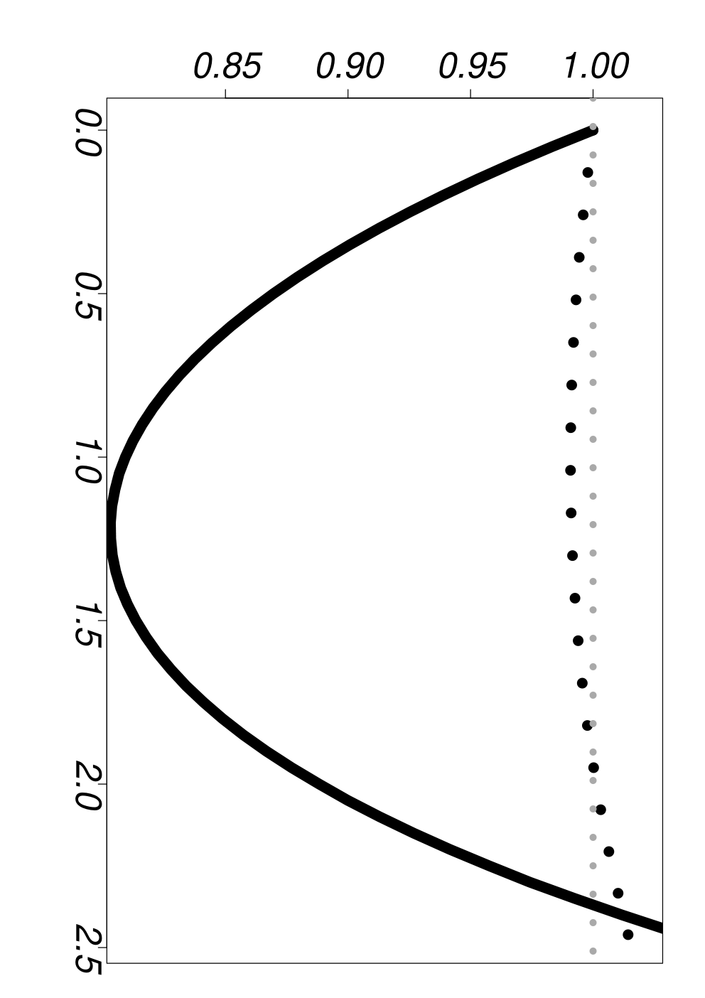
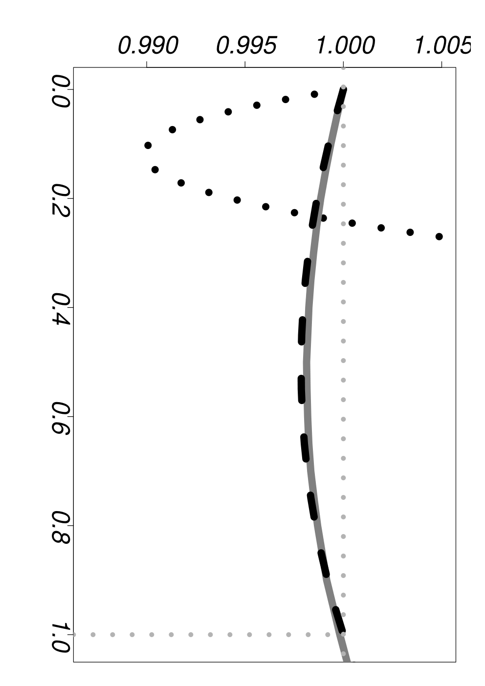
Figure 5 and Table 1 illustrate that , the sum of the meaningful GARCH parameters, has a substantial impact on the value of with for , we find ; when , then ; and for , , with the latter consistent with Theorem 3.4. Unfortunately, when no explicit relationship appears to hold between and , as changes markedly with the innovation distribution. From Table 1 is can be seen that when we have that the shorter the tail of the innovation distribution gives the larger and hence shorter tails of the GARCH marginal distribution; whereas the reverse holds when ; and when then is invariant to the innovation distribution. The case when is somewhat surprising as at first thought you would expect that having a heavier tail innovation would result in a heavier tailed GARCH process, whereas in fact the opposite occurs.
We finish with empirical diagnostic checks to illustrate that the derived value of is consistent with the observable tail of the GARCH() process. The observable tail can be derived from long run simulations. Specifically we compare the probabilities limiting with the empirical estimate of the probabilities for very large , over a range of . Figure 6 shows this comparison on a log scale. With the choice of such scaling the true relationship between them has a gradient . The results show that at this far into the distributional tail, and subject to Monte Carlo noise, the empirical distribution is consistent with the limit formulation, and hence also is consistent with the value for that we have derived.


5.7 Evaluation of
In Section 4 we introduced a tail-skewness parameter as a limiting conditional probability (4.1). We have not found any previous discussion on the evaluation of , which is an important parameter in the calculation of extremal features of GARCH() processes when the innovations are asymmetrically distributed, despite Ehlert et al. 2015 covering this class for GARCH(1,1) processes. A natural starting point to evaluate is to take a long-run simulation from the GARCH() process and simply estimate the probability (4.1) empirically for a large enough value of . However, this is likely to be unreliable in practice.
Key to the method we propose is the following expression
| (5.1) | |||||
where is the distribution of , the the component of the limit vector which is defined by limit (2.6).
For the innovation distribution then expression (5.1) becomes
With a sample of from derived using Algorithm 1 we can get a Monte Carlo approximation, to any desired accuracy though the choice of , as follows
Intuitively it seems as though should be equal to , where is the upper end point of . This is not the case though, as knowing that is large is quite different from knowing that is large, as the former also can be achieved with large volatility and small innovations. For we have that is given by
Figure 7 shows how varies with the skew- distribution parameter for ; the values of for follow due to being symmetrical about , i.e., for then is equal to . The figure shows that for a given level of , i.e., skewness in the innovation distribution, as increases there is a diminishing level of skewness in the tails of the GARCH process as measured by . When then , and this value is seen to be an upper bound for in Figure 7. These results are consistent with intuition as the larger the value of the more the process is driven by the past values of the process and the less the new innovations (and their skewness) matter. Table 1 illustrates how changes over models when , with typically decreasing as increases, as the persistence of volatility is more important than the innovation structure as increases.

6 Results for the GARCH() process
6.1 Extremogram
Figure 8 gives the extremogram for the squared of GARCH process for models A-D with normal and innovations with degrees of freedom. Firstly notice the impact of the innovation distribution on . In all cases the heavier tailed innovation distribution leads to weaker extremal dependence at all lags. Models C and D, both IGARCH processes (with ), exhibit much slower decay rates in extremal dependence as lag increases than for models A and B with , with the level of extremal dependence appearing to be strongly related to . Furthermore, we see for models B and D that , with decaying monotonically for . The reason for this seems to be that here. From Section 4 we have that the evaluation of and is simple from once is known, which we have from Section 5.7 and Table 1.
An empirical estimate of the extremogram of based on a sample of length from a GARCH() process is given by
where is a threshold. Figure 8 shows for large and for three threshold choices corresponding to and quantiles of . The agreement with limit values that we have evaluated is very good generally, with the empirical estimates suffering from bias and variance trade-off, as with all threshold based estimates. Model B has the slowest convergence of the empirical estimator, but even here at the highest threshold there is almost perfect overlap between empirical estimates and the true values for all lags . In contrast for model C the highest threshold produces the least good estimate, presumably due to its high variance. This gives strong evidence that our evaluation of is accurate, but it also shows how difficult it is to get accurate values from direct simulations due to different convergence rates from apparently rather similar models.


6.2 Extremal Index
We finish by looking at how the extremal index , and , of the upper tail of the series and , change over GARCH() processes. Results for each of these characteristics are given for models A-E and three innovation distributions are given in Table 1. Firstly consider the effect of the innovation distribution for a given model on the extremal index of the process, through the associated average size of clusters extremes values, i.e., . With shorter tailed innovations clusters last longer on average and introducing skewness further reduces the mean cluster size. For increasing , for , we have increasing average cluster sizes, but that pattern does not follow when . In all cases, , indicating the extremes of the processes and exhibit less clustering on average than the process. We have equality, in this inequality, only when or , and find that as tends to these limits one or other of the processes and has similar cluster of extremes events as the process. For more clustering occurs in the upper tail than in the lower tail of the GARCH process, with the reverse happening with .
To give a better idea of how the GARCH() parameters affect the extremal index Figure 9 presents a contour plot of for GARCH(2,2) process over different key parameters . In particular, in each panel we hold fixed two parameters and contour over the other two key parameters of a GARCH(2,2) process. Figure 9, shows that broadly decreases, i.e., average cluster sizes increase, with increasing , up to the boundary case of an IGARCH(2,2) model. Consequently contours are near linear in the parameters. Unless is large then small values of and tend to lead to very limited clustering. This seems logical given the GARCH formulation, as small and mean that the effect of the large value can have limited impact of the subsequent volatilities, so without and being large, to pick up the momentum of the evolution of the event, the large event is very likely to die out rapidly. We also have that we obtain stronger extremal dependence with larger values of the pair than for for equal values of , as seen by values of being smaller in Figure 9 right panel by comparison to the left panel. The reason for this is the stronger effect of coefficients compared to that of the as the persistency in the volatility is translated into a stronger extremal dependence.


.
7 Discussion
The new theory and methods we present extend to assessing the strict stationarity and extremal properties for a much broader class of stochastic recurrence equations. Specifically, for any process
where and are stochastic, independent and identically distributed, sequences of matrices and vectors respectively, satisfying the conditions of Kesten 1973, then our paper gives methods which: help assess stationarity of the process; determine its tail index of regular variation for the marginals distributions of ; determine ways to simulate from the spectral measure from the limiting joint distribution of given some norm, , tends to infinity; and are able to generate a wide range of properties, such as the extremal index of any marginal of the process from its tail chain. Previously none of these properties could be derived due to a combination of a lack of appropriate numerically stable algorithms. The methods presented here overcome these limitations and provide a broad toolbox of numerically robust approaches to derive the extremal analysis of a wide class of stochastic recurrence equations including all GARCH() processes with bounded and unbounded innovation variables.
Appendix A Proof of Theorems
Proof of Theorem 3.1.
First rewrite the product of independent matrices as
| (A.1) |
Thus
so as
hence . ∎
Proof of Theorem 3.2.
With the same notation as for Theorem 3.1 we have that
| (A.2) | |||||
Under condition (3.3) we have that there exists a sequence such that and as
for all . Combining these inequalities with expression (A.2) we obtain that
Focusing first on the upper bound we have that
where the second step comes from , being independent and identically distributed. Hence, as
By an identical argument, the lower bound is found to be asymptotically equal to the upper bound. Hence
so this limit is equal to 0, as required by condition (2.15), only when satisfies .
∎
Proof of Theorem 3.4.
First suppose that , then from property (2.13) we have that , where is independent of . Then, by considering the vector , we see that marginally the first and the last components of each have identical marginal distributions. Furthermore, as , it follows that all for all , where recall . We also have that
Let denote the th element of , using the independence of from then
Thus only when , i.e., when the process is IGARCH(). The argument is simply reversed giving that for any IGARCH() process. ∎
Acknowledgements
We would like to thank Feridun Turkman for encouraging and helpful discussions.
References
- Azzalini and Capitanio (2003) Azzalini, A. and Capitanio, A. (2003) Distributions generated by perturbation of symmetry with emphasis on a multivariate skew t-distribution. Journal of the Royal Statistical Society, Series B, 65, 367–389.
- Basrak et al. (2002) Basrak, B., Davis, R. A. and Mikosch, T. (2002) Regular variation of GARCH processes. Stochastic Processes and their Applications, 99, 95–115.
- Basrak and Segers (2009) Basrak, B. and Segers, J. (2009) Regularly varying multivariate time series. Stochastic Processes and their Applications, 119, 1055–1080.
- Basrak and Segers (2011) Basrak, B. and Segers, J. (2011) Erratum to: “Regularly varying multivariate time series” [Stochastic Process. Appl. 119 (2009) 1055–1080]. Stochastic Processes and their Applications, 121, 896 – 898.
- Bollerslev (1986) Bollerslev, T. (1986) Generalized autoregressive conditional heteroskedasticity. Journal of Econometrics, 31, 307–327.
- Bougerol and Picard (1992) Bougerol, P. and Picard, N. (1992) Stationarity of GARCH processes and of some nonnegative time series. Journal of Econometrics, 52, 115–127.
- Breidt and Davis (1998) Breidt, J. F. and Davis, R. A. (1998) Extremes of stochastic volatility models. The Annals of Applied Probability, 8, 664–675.
- Collamore et al. (2014) Collamore, J. F., Diao, G. and Vidyashankar, A. N. (2014) Rare event simulation for processes generated via stochastic fixed point equations. The Annals of Applied Probability, 24, 2143–2175.
- Davis and Mikosch (2009a) Davis, R. A. and Mikosch, T. (2009a) Extreme value theory for GARCH processes. In Handbook of Financial Time Series (eds. T. Andersen, R. Davis, J. Kreiss and T. Mikosch). New York: Springer, pp. 187–200.
- Davis and Mikosch (2009b) Davis, R. A. and Mikosch, T. (2009b) The extremogram: a correlogram for extreme events. Bernoulli, 4, 977–1009.
- de Haan et al. (1989) de Haan, L., Resnick, S. I., Rootzén, H. and de Vries, C. G. (1989) Extremal behaviour of solutions to a stochastic difference equation with applications to ARCH processes. Stochastic Processes and their Applications, 32, 213–224.
- Del Moral and Miclo (2000) Del Moral, P. and Miclo, L. (2000) Branching and interacting particle systems approximations of Feynman-Kac formulae with applications to non-linear filtering. In Seminaire de probabilites XXXIV. Springer, pp. 1–145.
- Del Moral and Miclo (2003) Del Moral, P. and Miclo, L. (2003) Particle approximations of Lyapunov exponents connected to Schrödinger operators and Feynman–Kac semigroups. ESAIM: Probability and Statistics, 7, 171–208.
- Doucet et al. (2000) Doucet, A., Godsill, S. and Andrieu, C. (2000) On sequential Monte Carlo sampling methods for Bayesian filtering. Statistics and Computing, 10, 197–208.
- Ehlert et al. (2015) Ehlert, A., Fiebig, U.-R., Janssen, A. and Schlather, M. (2015) Joint extremal behavior of hidden and observable time series with applications to GARCH processes. Extremes, 18, 109–140.
- Francq and Zakoïan (2010) Francq, C. and Zakoïan, J.-M. (2010) GARCH Models: Structure, Statistical Inference and Financial Applications. Chichester, United Kingdom: John Wiley & Sons, Ltd.
- Goldsheid (1991) Goldsheid, I. Y. (1991) Lyapunov exponents and asymptotic behaviour of the product of random matrices. Lecture Notes in Mathematics, 1486, 23–37.
- Griffin et al. (2017) Griffin, A., Jenkins, P. A., Roberts, G. O. and Spencer, S. E. (2017) Simulation from quasi-stationary distributions on reducible state spaces. Advances in Applied Probability, 49, 960–980.
- Hsing et al. (1988) Hsing, T., Hüsler, J. and Leadbetter, M. R. (1988) On the exceedance point process for a stationary sequence. Probability Theory and Related Fields, 78, 97–112.
- Janssen (2010) Janssen, A. (2010) On Some Connections between Light Tails, Regular Variation and Extremes. Ph.D. thesis, University of Gottingen.
- Janssen and Segers (2014) Janssen, A. and Segers, J. (2014) Markov tail chains. Journal of Applied Probability, 51, 1133–1153.
- Kallemberg (1983) Kallemberg, O. (1983) Random Measures. Berlin: Akademic-Verlag, 3rd edn.
- Kesten (1973) Kesten, H. (1973) Random difference equations and renewal theory for products of random matrices. Acta Mathematica, 131, 207–248.
- Kesten and Spitzer (1984) Kesten, H. and Spitzer, F. (1984) Random difference equations and renewal theory for products of random matrices. Zeitschrift für Wahrscheinlichkeitstheorie und Verwandte Gebiete, 67, 363–386.
- Laurini and Tawn (2012) Laurini, F. and Tawn, J. A. (2012) The extremal index for GARCH(1, 1) processes. Extremes, 15, 511–529.
- Ledford and Tawn (2003) Ledford, A. W. and Tawn, J. A. (2003) Diagnostics for dependence within time series extremes. Journal of the Royal Statistical Society, Series B, 65, 521–543.
- Mikosch and Stărică (2000) Mikosch, T. and Stărică, C. (2000) Limit theory for the sample autocorrelations and extremes of a GARCH(1,1) process. The Annals of Statistics, 28, 1427–1451.
- O’Brien (1987) O’Brien, G. L. (1987) Extreme values for stationary and Markov sequences. The Annals of Probability, 15, 281–291.
- Planinić and Soulier (2018) Planinić, H. and Soulier, P. (2018) The tail process revisited. Extremes, 21, 551–579. URL https://doi.org/10.1007/s10687-018-0312-1.
- Resnick (1987) Resnick, S. I. (1987) Extreme Values, Regular Variation, and Point Processes. New York: Springer-Verlag.
- Rootzén (1988) Rootzén, H. (1988) Maxima and exceedancs of stationary Markov chains. Advanced in Applied Probability, 20, 371–390.
- Segers (2003) Segers, J. (2003) Functionals of clusters of extremes. Advances in Applied Probability, 35, 1028–1045.
- Smith et al. (1997) Smith, R. L., Tawn, J. A. and Coles, S. G. (1997) Markov chain models for threshold exceedances. Biometrika, 84, 249–268.
- Smith and Weissman (1994) Smith, R. L. and Weissman, I. (1994) Estimating the extremal index. Journal of the Royal Statistical Society, Series B, 56, 515–528.
- Taylor (1986) Taylor, S. J. (1986) Modelling Financial Time Series. Chichester: Wiley.