Simple formula for integration of polynomials on a simplex Journal: BITThanks: Research funded by the European Research Council (ERC) under the European’s Union Horizon 2020 research and innovation program (grant agreement 666981 TAMING)

In addition to being a mathematical problem of independent interest, integrating a polynomial on a polytope has important applications in e.g. computational geometry, in approximation theory (constructing splines), in finite element methods, to cite a few; see e.g. the discussion in Baldoni et al. baldoni. In particular, because of applications in finite (and extended finite) element methods and also for volume computation in the Natural Element Method (NEM), there has been a recent renewal of interest in developing efficient integration numerical schemes for polynomials on convex and non-convex polytopes

For instance the HNI (Homogeneous Numerical Integration) technique developed in Chin et al. chin and based on lass-poly, has been proved to be particular efficient in some finite (and extended finite) element methods; see e.g. Antonietti et al. galerkin, Chin and Sukumar suku, Nagy and Benson nagy for intensive experimentation, Zhang et al. zhang for NEM, Frenning frenning for DEM (Discrete Element Method), Leoni and Shokef leoni for volume computation. For exact volume computation of polytopes in computational geometry, the interested reader is also referred to Büeler et al. bueler and references therein.

For integrating a polynomial on a polytope, one possible route is to use the HNI method developed in lass-poly; chin and also extended in galerkin, without partitioning the polytope in simplices. Another direction is to consider efficient numerical schemes for simplices since quoting Baldoni et al. baldoni “among all polytopes, simplices are the fundamental case to consider for integration since any convex polytope can be triangulated into finitely many simplices”. In baldoni the authors analyze the computational complexity of the latter case and describe several formulas; in particular they show that the problem is NP-hard in general. However, if the number of variables is fixed then one may integrate polynomials of linear forms efficiently (with Straight-Line program for evaluation) and if the degree is fixed one may integrate any polynomial efficiently. They also describe several formulas in closed form for integrating powers of linear forms (baldoni, Corollary 12) and also arbitrary homogeneous polynomials (baldoni, Proposition 18) and lass-avra, all stated in terms of a summation over vertices of the simplex.

With $f\in\mathbb{R}[\mathbf{x}]$, $\mathbf{x}\mapsto f(\mathbf{x})=\sum_{\alpha}f_{\alpha}\,\mathbf{x}^{\alpha}$ is associated the Bombieri-type polynomial $\hat{f}\in\mathbb{R}[\mathbf{x}]$:

We establish the following simple formula:

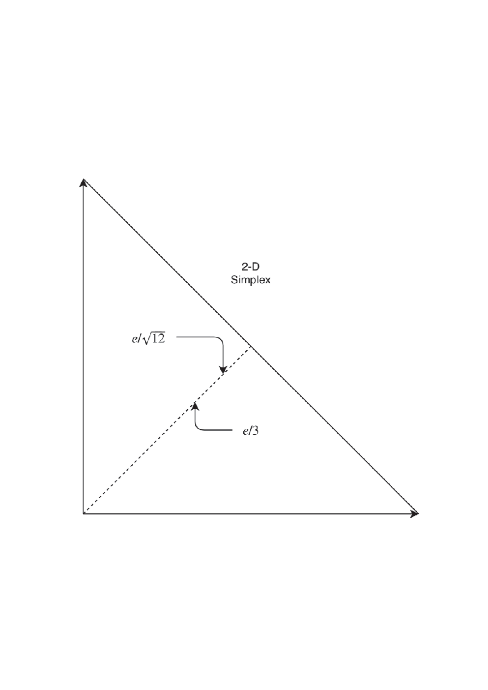
Theorem 1.1 states that integrating a polynomial $f$ of degree $t$ on the canonical simplex $\boldsymbol{\Delta}$ can be done by evaluating each Bombieri form $\hat{f}_{j}$ at a unique point $\boldsymbol{\xi}_{j}\in\boldsymbol{\Delta}$. In addition all points $(\boldsymbol{\xi}_{j})$ are on a line between the origin and the point $\mathbf{e}/n$ on the boundary of $\boldsymbol{\Delta}$. To the best of our knowledge, and despite their simplicity, we have not been able to find formula (2) or (4) in the literature, even if they can be obtained in several relatively straightforward manners from previous results in the literature.

The point that we make in (2) is to relate $\int_{\boldsymbol{\Delta}}\,f\,d\mathbf{x}$ to point evaluation of its Bombieri-polynomial at only $t$ very specific points of the simplex $\boldsymbol{\Delta}$; and similarly for positively homogeneous functions of the form (3).

Similarly, integrating a polynomial $f$ of degree $t$ on an arbitrary simplex $\boldsymbol{\Omega}\subset\mathbb{R}^{n}$ can be done by evaluating related polynomials $h_{j}$ of degree $j$, each at a certain point of $\boldsymbol{\Omega}$. Indeed an arbitrary (full-dimensional) simplex can be mapped to the canonical simplex $\boldsymbol{\Delta}$ by an affine transformation $\mathbf{y}=\mathbf{A}\,(\mathbf{x}-\mathbf{a})$ for some real nonsingular matrix $\mathbf{A}$ and vector $\mathbf{a}\in\mathbb{R}^{n}$. Therefore (2) translates to a similar formula on $\boldsymbol{\Omega}$ with ad-hoc polynomials and $t$ aligned points $\mathbf{x}_{j}\in\boldsymbol{\Omega}$.

Hence formula (2) is much simpler than those in baldoni; lass-avra. In particular it is valid for an arbitrary polynomial and there are only $t$ points involved if the degree of the polynomial is $t$. In contrast, for integrating a $t$-power of a linear form, the formula in baldoni requires a summation at the $(n+1)$ vertices and in lass-avra, integrating a form of degree $t$ requires ${n+t\choose n}$ evaluations of a multilinear form at the $(n+1)$ vertices.

We would like to emphasize that (2) resembles a cubature formula but is not. A cubature formula is of the form:

for some integer $s$ and points $(\mathbf{x}_{j})\subset\boldsymbol{\Delta}$ with associated weights $w_{j}$, $j=1,\ldots,s$. However Theorem 1.1 suggests that as long as polynomials are concerned, the simpler alternative formula (2) could be preferable to cubature formulas involving many points. The point of view is different. Instead of evaluating the single polynomial $f$ of degree $t$ at several points $\mathbf{x}_{j}$ in (5), in (2) one evaluates $t$ other polynomials $\hat{f}_{j}$ of degree $j$, $j=1,\ldots t$ (simply related to $f$); each polynomial $\hat{f}_{j}$ is evaluated at a single point only.

Our technique of proof is relatively simple. It uses (i) Laplace transform technique and homogeneity to reduce integration on $\boldsymbol{\Delta}$ with respect to (w.r.t.) Lebesgue measure to integration on the nonnegative orthant w.r.t. exponential density; this technique was already advocated in lass-zeron for computing certain multivariate integrals and in volume for volume computation of polytopes. Then (ii) integration of monomials w.r.t. exponential density can be done in closed-form and results in a simple formula in closed form.

Interestingly and somehow related, recently Kozhasov et al. sturmfels have considered integration of a “monomial” $\mathbf{y}^{\alpha-\mathbf{e}}$ (with $0<\alpha\in\mathbb{R}^{n}$) with respect to exponential density on the positive orthant. In sturmfels the density $\mathbf{y}\mapsto\prod_{i}\Gamma(\alpha_{i})\,y_{i}^{\alpha_{i}-1}$ is called the Riesz kernel of the monomial $\mathbf{x}^{-\alpha}$. The Riesz kernel offers a certificate of positivity for a function to be completely monotone (a strong positivity property of functions on cones).

Let $\mathbb{R}[\mathbf{x}]$ denote the ring of real polynomials in the variable $\mathbf{x}=(x_{1},\ldots,x_{n})$. With $\mathbb{N}$ the set of natural numbers, a polynomial $f\in\mathbb{R}[\mathbf{x}]$ is written

in the canonical basis of monomials. A polynomial $f$ is homogeneous of degree $t$ if $f(\lambda\,\mathbf{x})=\lambda^{t}\,f(\mathbf{x})$ for all $\lambda\in\mathbb{R}$ and all $\mathbf{x}\in\mathbb{R}^{n}$. For $\alpha\in\mathbb{R}^{n}$ let $|\alpha|:=\sum_{i}|\alpha_{i}|$. Let $\mathbb{R}^{n}_{+}:=\{\mathbf{x}\in\mathbb{R}^{n}:\mathbf{x}\geq 0\}$ denotes the positive orthant of $\mathbb{R}^{n}$. A function $f:(\mathbb{R}_{+}\setminus\{0\})^{n}\to\mathbb{R}$ is positively homogeneous of degree $t\in\mathbb{R}$ if

and a polynomial $f$ is homogeneous of degree $t\in\mathbb{R}$ if

Denote by $\boldsymbol{\Delta}\subset\mathbb{R}^{n}_{+}$ the canonical simplex $\{\mathbf{x}\in\mathbb{R}^{n}_{+}:\mathbf{e}^{T}\mathbf{x}\leq 1\}$ where $\mathbf{e}=(1,\ldots,1)\in\mathbb{R}^{n}$. For $0<\mathbf{x}\in\mathbb{R}^{n}$ let $1/\mathbf{x}=(\frac{1}{x_{1}},\ldots,\frac{1}{x_{n}})\in\mathbb{R}^{n}$.

With a polynomial $f\in\mathbb{R}[\mathbf{x}]$ in (6) is associated the “Bombieri” polynomial:

After an affine transformation, integrating $f$ on an arbitrary full-dimensional simplex $\boldsymbol{\Omega}\subset\mathbb{R}^{n}$ reduces to integrating a related polynomial of same degree on the canonical simplex $\boldsymbol{\Delta}=\{\mathbf{x}\in\mathbb{R}^{n}_{+}:\mathbf{e}^{T}\mathbf{x}\leq 1\}$ where $\mathbf{e}=(1,\ldots,1)\in\mathbb{R}^{n}$. Therefore in this section we consider integrals of polynomials (and a certain type of positively homogeneous functions) on the canonical simplex $\boldsymbol{\Delta}$.

As the reader can see, formula (10) is extremely simple and only requires evaluating $\hat{f}$ at the unique point $\boldsymbol{\xi}_{t}\in\boldsymbol{\Delta}$. This in contrast to the formula in lass-avra which requires a sum of ${n+t\choose n}$ terms, each involving evaluations at the vertices of $\boldsymbol{\Delta}$.

Hence from Remark 1, with $C=(\mathbb{R}\setminus\{0\})^{n}$ and $d\mu=fd\mathbf{x}$, we obtain:

Proposition 1 is in the spirit of sturmfels[Proposition 2.7]. Next given $\boldsymbol{\ell},\mathbf{x}\in\mathbb{R}^{n}$ denote by $\boldsymbol{\ell}\cdot\mathbf{x}$ the scalar product $\boldsymbol{\ell}^{T}\mathbf{x}$ and by $\boldsymbol{\ell}\otimes\mathbf{x}\in\mathbb{R}^{n}$ the vector $(\ell_{1}x_{1},\ldots,\ell_{n}x_{n})$. Finally let $\mathrm{E}_{t}\in\mathbb{R}[\mathbf{x}]$ the homogeneous polynomial of degree $t$ with all coefficients equal to $1$, that is, $\mathbf{x}\mapsto\mathrm{E}_{t}(\mathbf{x}):=\sum_{|\alpha|=t}\mathbf{x}^{\alpha}$.

As a consequence of Theorem 2.1 we obtain:

Hence Corollary 1 states that integrating $f$ on $\boldsymbol{\Delta}$ reduces to evaluate each $\hat{f}_{j}$ at the unique point $\boldsymbol{\xi}_{j}\in\boldsymbol{\Delta}$, and sum up. In addition, all points $\boldsymbol{\xi}_{j}$, $j=1,\ldots,t$, are aligned in $\boldsymbol{\Delta}$; they are between the origin $0$ and the point $\mathbf{e}/n\in\boldsymbol{\Delta}$, on the line joining $0$ to $\mathbf{e}/n$. Again formula (13) and (14) are extremely simple. The former only requires evaluating $\hat{f}_{j}$ at $\boldsymbol{\xi}_{j}$ ($t$ evaluations) and the latter only requires evaluating the polynomial $\mathrm{E}_{t}$ at the point $\boldsymbol{\ell}\in\mathbb{R}^{n}$. This is contrast with (baldoni, Corollary 12, p. 307) which is more complicated (even for a single form $\ell$).

Finally, Theorem 2.1 can be extended to a class of homogeneous functions

Let $\boldsymbol{\Omega}\subset\mathbb{R}^{n}$ be an arbitrary full-dimensional simplex (its $n$-dimensional Lebesgue volume is strictly positive). Then $\boldsymbol{\Omega}$ is mapped to $\boldsymbol{\Delta}$ by some affine transformation. In a fixed basis, this is obtained by the change of variable $\mathbf{y}:=\mathbf{A}(\mathbf{x}-\mathbf{a})$ where $\mathbf{A}$ is one non singular $n\times n$ real matrix and where $\mathbf{a}\in\mathbb{R}^{n}$ is a vertex of $\boldsymbol{\Omega}$. Then:

Next, if $f$ is a polynomial of degree $t$:

where $g$ has same degree as $f$. Next, writing $g=\sum_{j=0}^{t}g_{j}(\mathbf{y})$ with $g_{j}$ homogeneous of degree $j$, one has

and therefore with $\boldsymbol{\xi}_{j}\in\boldsymbol{\Delta}$ as in Corollary 1, $\boldsymbol{\psi}_{j}:=\mathbf{A}^{-1}\boldsymbol{\xi}_{j}+\mathbf{a}\in\boldsymbol{\Omega}$ and $\hat{g}_{j}(\boldsymbol{\xi}_{j})=\hat{g}_{j}(\mathbf{A}(\boldsymbol{\psi}_{j}-\mathbf{a}))$. Therefore combining (16) and (13) in Corollary 1 yields:

the analogue for $\boldsymbol{\Omega}$ of (13) for $\boldsymbol{\Delta}$.

In addition, let $f$ be homogeneous of degree $t$ with Waring-like decomposition³³ 3 In number theory, the Waring problem consists of writing any positive integer as a sum of a fixed number $g(n)$ of $n$th powers of integers, where $g(n)$ depends only on $n$. It generalizes to forms as a generic form of degree $d$ can be written as a sum of $s$ $d$-powers of linear forms; $s$ is called the Waring rank of the form.

for finitely many $\mathbf{c}_{i}\in\mathbb{R}^{n}$ and $\varepsilon_{i}\in\{-1,1\}$, $i=1,\ldots,s$. Then letting $\boldsymbol{\ell}_{i}=(\mathbf{A}^{-1})^{T}\mathbf{c}_{i}$:

where we have used Newton binomial formula and Corollary 1(ii) (and recall that $\mathrm{E}_{k}(\mathbf{x})=\sum_{|\alpha|=k}\mathbf{x}^{\alpha}$). In particular, if $\mathbf{a}=0$ and now with $\boldsymbol{\ell_{i}}:=(\mathbf{A}^{-1})^{T}\mathbf{c}_{i}$, $i=1,\ldots,s$, it simplifies to

References

• (1) Antonietti P. F., Houston P., Pennesi G., Fast Numerical Integration on Polytopic Meshes with Applications to Discontinuous Galerkin Finite Element Methods, J. Sci. Comp., 77, pp. 339–1370 (2018).
• (2) Baldoni V., Berline N., De Loera J.A., Köppe M., Vergne M. How to integrate a polynomial over a simplex, Math. Comput., 80, pp. 297–325 (2011).
• (3) Büeler B., Enge A., Fukuda K., Exact volume computation for polytopes: A practical study. In Gil Kalai and Günter M. Ziegler, editors, Polytopes – Combinatorics and Computation, volume 29 of DMV Seminar, pages 131–154. Birkhäuser Verlag, Basel (2000).
• (4) Chin E.B., Lasserre J.B., Sukumar N., Numerical integration of homogeneous functions on convex and nonconvex polygons and polyhedra, Comput. Mech., 56, pp. 967–981 (2015).
• (5) Chin E. B., Sukumar N., Modeling curved interfaces without element-partitioning in the extended finite element method, Int. J. Num. Methods Eng. to appear. https://doi.org/10.1002/nme.6150
• (6) Frenning G., Efficient Voronoi volume estimation for DEM simulations of granular materials under confined conditions, MethodsX 2, pp. e79-e90 (2015).
• (7) Kozhasov K., Michalek M., Sturmfels B., Positivity certificates via integral representations, arXiv:1908.04191 (2019).
• (8) Lasserre J.B., Avrachenkov, K., The multi-dimensional version of ∫abxp​𝑑x\int_{a}^{b}x^{p}dx. Amer. Math. Monthly, 108, pp. 151–154 (2001).
• (9) Lasserre J.B., Zeron, E.S., Solving a class of multivariable integration problems via Laplace Lechniques, Appl. Math. (Warsaw), 28, pp. 391–405 (2001).
• (10) Lasserre J.B., Zeron E.S., A Laplace transform algorithm for the volume of a convex polytope Journal of the ACM, 48, pp. 1126–1140 (2001).
• (11) Lasserre, J.B., Integration on a convex polytope, Proc. Am. Math. Soc., 126, pp. 2433–2441(1998).
• (12) Leoni F., Yair Shokef Y., Attraction Controls the Inversion of Order by Disorder in Buckled Colloidal Monolayers, Phys. Rev. Letters (2017).
• (13) Nagy A.P., Benson D.J., On the numerical integration of trimmed isogeometric elements, Comput. Methods Appl. Mech. Eng., 284, pp. 165–185 (2015).
• (14) Yong Zhang, Yu Ma, Hong-Liang Yin, He-Ping Tan, Natural element method for solving radiative transfer with or without conduction in three-dimensional complex geometries, J. Quantitative Spectroscopy & Radiative Transfer, 129, pp. 118–130 (2013).