Random-effects meta-analysis
of phase I dose-finding studies
using stochastic process priors
2 F-CRIN Partners Platform, Paris, France
3 University Medical Center Göttingen, Göttingen, Germany
August 1, 2019
Abstract
Phase I dose-finding studies aim at identifying the maximal tolerated dose (MTD). It is not uncommon that several dose-finding studies are conducted, although often with some variation in the administration mode or dose panel. For instance, sorafenib (BAY 43-900) was used as monotherapy in at least 29 phase I trials according to a recent search in clinicaltrials.gov. Since the toxicity may not be directly related to the specific indication, synthesizing the information from several studies might be worthwhile. However, this is rarely done in practice and only a fixed-effect meta-analysis framework was proposed to date. We developed a Bayesian random-effects meta-analysis methodology to pool several phase I trials and suggest the MTD. A curve free hierarchical model on the logistic scale with random effects, accounting for between-trial heterogeneity, is used to model the probability of toxicity across the investigated doses. An Ornstein-Uhlenbeck Gaussian process is adopted for the random effects structure. Prior distributions for the curve free model are based on a latent Gamma process. An extensive simulation study showed good performance of the proposed method also under model deviations. Sharing information between phase I studies can improve the precision of MTD selection, at least when the number of trials is reasonably large.
1 Introduction
Phase I dose-finding studies are carried out during early stages of the clinical development, and aim at estimating the maximum tolerated dose (MTD) of a drug or a combination of molecules. The MTD is defined with reference to the occurrence of treatment-related adverse events, so-called dose-limiting toxicities (DLTs). The MTD then is reached once the rate of DLTs exceeds an acceptable level. Phase I studies are usually done on small numbers of healthy volunteers, except in oncology, where, due to the potentially high toxicity of drugs, phase I trials are commonly performed on patients (Chevret 2006).
In oncology, identifying the correct or reasonable dose or set of doses is a crucial objective in the drug development process: selecting too high a dose means exposing patients to an unacceptable toxicity profile, while selecting a dose of too low toxicity increases the likelihood that the treatment provides insufficient efficacy (Bretz et al. 2005). The dose escalation paradigm in phase I (or I/II) trials thus generally aims to avoid recommending too toxic doses of an agent while maintaining an acceptable toxicity. Due to limited sample sizes, conventional statistical methods are often inaccurate, so that adaptive sequential analyses have been proposed, as these can potentially find the MTD sooner and limit the number of exposed subjects (Le Tourneau et al. 2009; Neuenschwander et al. 2015).
When combining data across trials, two sources of potential heterogeneity need to be considered. Firstly, these are differences in the outcomes of the control groups. In the context of dose-escalation studies, there might be differences in the (true) toxicity probabilities due to variations in e.g. the study populations or in the definition and assessment of toxicities. Secondly, the (true) treatment effects, even if defined on a relative scale, might vary across trials. In standard meta-analysis models, the former is addressed by stratification for study. In so-called random-effects meta-analyses, the latter is addressed by inclusion of random study-by-treatment interactions. In fixed-effect or common-effect meta-analysis, a homogeneous treatment effect across trials is assumed. For a recent discussion of the various statistical models we refer here to Jackson et al. 2018. As evidenced by large-scale empirical investigations, some level of between-study heterogeneity is not unlikely to occur (Turner et al. 2012). However, estimation of the corresponding variance component and accounting appropriately for the uncertainty in estimation in inference of relevant model parameters can be challenging, if the number of studies included in the meta-analysis is small (Friede et al. 2017). In the context of meta-analyses of dose-escalation trials, we are still lacking an understanding as well as empirical evidence how the various forms of between-trial heterogeneity can be appropriately accounted for.
Zohar et al. 2011 proposed a meta-analysis approach for phase I clinical trials in oncology. Phase I data were pooled while accounting for the sequential nature of such trials in order to better estimate the overall MTD. However, this method did not deal with several important characteristics associated with phase I features. Firstly, data were pooled under several different administration schedules, which may imply different toxicity profiles. Secondly, between-trial heterogeneity was not taken into account, which may lead to inaccurate inference. Thirdly, as the pooled analysis was done retrospectively, it would have been possible to take into account cycles, dose-modifications and long term toxicities in order to better investigate the maximal dose regimen, but these complexities were not addressed.
Thomas et al. 2014 reported the results of a meta-analysis based on dose-response studies conducted by a large pharmaceutical company between 1998 and 2009. Data collection targeted efficacy endpoints, but safety data were not extracted. The goal of this meta-analysis was to identify consistent quantitative patterns in dose-response across different compounds and diseases. The meta-analysis excluded oncology trials as these have different dosing objectives and methods.
In this manuscript, we develop a novel meta-analysis approach for phase I clinical trials in oncology, which takes into account the different features described above to better suit the requirements in estimating MTDs. We generalized the binomial-normal hierarchical model (BNHM), which is most commonly used in the literature for meta-analysis of studies involving a single dose. In the following section, two motivating examples are described. In Section 3, the methodology is presented, along with prior distributions and different variations of MTD definitions. In Section 4 we describe model variations and simulation settings that we used to test the developed method and its sensitivity to varying circumstances. Finally, in Section 5, the new methodology is applied to the motivating case studies and some limitations are discussed in Section 6.
2 Motivating examples
Some might believe that there are more phase III than phase I studies, and so meta-analyses have largely focused on late-stage trials whereas opportunities in pooling phase I results have rarely been investigated. Furthermore, as phase I studies usually have small sample sizes and are mostly algorithm-based and only lately model based designs, methodologists have been less inclined to embrace this issue. The first illustration concerns sorafenib (BAY 43-9006) which is a kinase inhibitor approved for the treatment of advanced renal cell carcinoma, hepatocellular carcinoma, and radioactive iodine resistant advanced thyroid carcinoma. A search of the clinicaltrials.gov registry of clinical trials at the end of June 2019 revealed that there are at least 833 studies using sorafenib (at any recruitment stage and type of study) of which 248 studies were labeled as “phase I” or “phase I/II” and 99 studies were labeled as “phase III” or “phase II/III”. Of 248 phase I or phase I/II studies using sorafenib, 29 studies used it in phase I as monotherapy (median sample size 22, range 2–158).
Today, the dose recommended by the European Medicines Agency (EMA) is 400 milligrams (mg) twice a day. Several phase I studies on sorafenib monotherapy have been performed, and some of their results are summarized in Table 1. Within these 14 trials, a total of 7 doses were tested, with most of these studies targeting solid tumors or leukemia. DLT definitions were comparable, and most of sorafenib schedules followed a 28-day cycle or similar.
| Dose (mg) | |||||||
|---|---|---|---|---|---|---|---|
| Study | 100 | 200 | 300 | 400 | 600 | 800 | 1000 |
| Clark et al. 2005 | 0/3 | 0/3 | 1/4 | 1/6 | 3/3 | ||
| Awada et al. 2005 | 0/4 | 0/3 | 1/5 | 1/10 | 7/12 | 1/3 | |
| Moore et al. 2005 | 0/3 | 1/6 | 0/8 | 3/7 | |||
| Strumberg et al. 2005 | 1/5 | 1/6 | 0/15 | 4/14 | 2/7 | ||
| Minami et al. 2008 | 0/3 | 1/12 | 0/6 | 1/6 | |||
| Miller et al. 2009 | 8/34 | 6/20 | |||||
| Nabors et al. 2011 | 0/3 | 1/6 | 0/3 | 1/5 | 3/3 | ||
| Chen et al. 2014 | 0/3 | 1/16 | |||||
| Jia et al. 2013 | 3/4 | ||||||
| Borthakur et al. 2011-1 | 0/3 | 0/15 | 2/8 | ||||
| Borthakur et al. 2011-2 | 0/3 | 1/7 | 2/6 | ||||
| Crump et al. 2010-1 | 0/4 | 1/6 | 0/6 | 1/6 | |||
| Crump et al. 2010-2 | 0/3 | 1/6 | 0/3 | 2/6 | |||
| Furuse et al. 2008 | 0/12 | 1/14 | |||||
Applying the common-effect approach proposed by Zohar et al. 2011 (in the following referred to as the ZKO approach) to the sorafenib data (Table 1) and using as skeleton, that is the set of prior toxicity probabilities for the doses (chosen in a reasonable shape according O’Quigley and Zohar 2010 and Zohar et al. 2011), the following estimated toxicity probabilities are obtained: (0.012, 0.033, 0.093, 0.169, 0.308, 0.471, 0.53). Following the ZKO approach, and assuming a toxicity threshold of 0.33, a dose of 600 mg is estimated as MTD, while for a threshold of 0.2, the MTD is at 400 mg.
The second example concerns a combination therapy of irinotecan and S-1 (S-1 refers to a combination of three pharmacological compounds, namely tegafur, gimeracil, and oteracil potassium). Irinotecan is a topoisomerase 1 inhibitor. It has proven effective in combination with 5-fluorouracil (5-FU) but was associated with many adverse events. This is why the association with S-1 instead of 5-FU was evaluated. In this case 11 studies were used (Table 2) in which 10 doses were evaluated across all trials.
Applying the ZKO method on the S-1 data (Table 2) and using (0.005, 0.05, 0.1, 0.2, 0.3, 0.4, 0.5, 0.6, 0.65, 0.70) as skeleton we obtain the following estimated toxicity probabilities: (0.002, 0.026, 0.061, 0.141, 0.231,0.328, 0.43, 0.537, 0.592, 0.648). Assuming a toxicity threshold of 0.33, dose 90 mg/m2 is estimated as MTD, while for a threshold of 0.2, the MTD is at 80 mg/m2.
| Dose (mg/m2) | ||||||||||
| Study | 40 | 50 | 60 | 70 | 80 | 90 | 100 | 120 | 125 | 150 |
| Ogata et al. 2009 | 0/3 | 0/3 | 3/4 | |||||||
| Inokuchi et al. 2006 | 0/3 | 10/42 | 0/3 | 2/3 | ||||||
| Goya et al. 2012 | 0/3 | 0/3 | 3/5 | |||||||
| Takiuchi et al. 2005 | 1/6 | 0/3 | 0/4 | 3/6 | ||||||
| Ishimoto et al. 2009 | 0/3 | 0/3 | 0/3 | 2/4 | ||||||
| Kusaba et al. 2010 | 0/6 | 2/3 | ||||||||
| Nakafusa et al. 2008 | 7/39 | 2/3 | ||||||||
| Shiozawa et al. 2009 | 1/6 | 2/6 | 2/6 | 2/3 | ||||||
| Yoda et al. 2011 | 0/3 | 3/6 | ||||||||
| Komatsu et al. 2010 | 1/9 | 1/9 | 0/3 | |||||||
In the two examples given above, not all trials shared the same doses, dose ranges and sample size. The ZKO method was applied to estimate the overall MTD. However, this is a simplistic way of pooling several adaptive sequential phase I data sets and it can be seen as a fixed-effect meta-analysis method. In the next section will be detailed our proposition taking into account these specificities as well as inter and intra trial heterogeneity by developing a non-parametric random-effects approach.
3 Methods
3.1 The dose-response model
In case of studies concerned with only a single dose, the binomial-normal hierarchical model (BNHM), or an approximation, is most commonly used in the literature (Jackson et al. 2018; Günhan et al. 2019). When moving to several doses in the same study, we propose an extension of the BNHM that is adapted to the dose-finding context, and that is able to also account for the ordering and spacing among doses.
Let be the study index, and be the dose level index, where all doses used in all trials are indexed in increasing order. Especially with data combined from several studies, the dose steps, that is the “spacing” between neighbouring doses , may be rather different (see e.g. the irinotecan example in Table 2) and needs to be accounted for in the model. We define as the metric, specifying the spatial proximity or distance between doses. This may simply be defined as the plain difference (). However, in many cases it may make sense to rather consider relative differences between dose levels on the logarithmic scale (). Another option may be to assume unit increments for neighbouring doses.
The number of patients in study allocated to dose is given by , while is the number of patients experiencing a DLT. We then propose the following model:
| (1) | |||||
| (2) |
where is the probability of toxicity of dose in the th study. The probabilities here are modelled on the logit-scale, with .
The fixed effects and (for ) are common across all studies; the summation in (2) ensures non-decreasing overall mean probabilities of toxicity with increasing dose. The random effects accounting for between-study heterogeneity are represented by the (study-specific) vectors , where represents the zero vector of dimension and the variance-covariance matrix. In order to meaningfully generalize from the BNHM for a single dose to a joint model for multiple doses, we specify the fixed and random effects accounting for the corresponding dose levels () and their ordering and proximity.
3.2 Gaussian process for the random effects
For the random effects, we specify a model that accounts for the position of dose on the dose continuum. We do not impose monotonicity here and we rely on a relatively simple class of Gaussian processes. Two interesting special cases are encompassed by the model, namely independent and identical residuals at all doses. In between these extremes, we utilize a stationary Ornstein-Uhlenbeck process (OUP) with covariance
| (3) |
where is the marginal variance, and is a smoothness parameter determining how quickly the autocorrelation decays and residuals become less dependent, depending on the spatial separation of doses. On small scales (relative to ), the OUP behaves like a Wiener process (or Brownian motion); this nicely corresponds with the notion that if we knew the residual at a certain dose, we knew less about the neighbouring residual the further we moved away from that dose, where increments behaved (approximately) additively, as for the fixed effects model introduced below. For the limiting cases of and it yields independent or identical residuals across doses, respectively (Uhlenbeck and Ornstein 1930; Doob 1942). Prior distributions for the random effect’s marginal variance and the OUP’s spatial scale need to be specified.
3.3 Gamma process for fixed effects prior distributions
The definition of the common effect via a sum of unknown increments in (2) places the model into the class of stochastic processes, which are commonly used as nonparametric models for unkown functions (Gelman et al. 2014, Ch. 21). Therefore, the prior distributions on the unknown increments may be inspired by a stochastic process. A natural and convenient class of models is defined via infinitely divisible probability distributions (Steutel 1979); that means that we stay within the same distribution class for the increments (i.e., if we sum two increments, the sum’s distribution again is within the same distribution class), which results in an overall consistent model. Since in the present case we are considering strictly positive increments for increasing doses, the Gamma process is an obvious choice here (Lawless and Crowder 2004).
The Gamma distribution is defined through two parameters, namely the shape and the scale ; its expectation then is and the variance is . Choosing the first dose () as the reference dose, we can specify the prior distributions as a Gamma process with
| (4) | |||||
| (5) |
where is the dose increment from dose to . To note, can be equal to (used in the specification of the random effects), or it can use another underlying metric. The parameter serves as an “intercept” term, and hyperparameters and then need to be specified with reference to the expected toxicity at the reference dose. The Gamma process hyperparameters and also need to be pre-specified. For a sensible choice, it is convenient to consider their effect on the conditional distribution for a unit increment:
| (6) | |||||
| (7) |
which suggests a re-parametrisation in terms of
| (8) | |||||
| (9) |
From this, we can see that for small , the (logit-) toxicity behaves approximately linear, while larger values allow for departures from linearity. In the limiting case of linearity, the model simplifies to a logistic model, which, in the special case of dose increments defined on the logarithmic scale as suggested above, again is a special case of the Emax model (Schwinghammer and Kroboth 1988).
3.4 Prior effective sample sizes for fixed effects
In order to assess how informative certain choices of priors and hyperprior parameters for the fixed effect are, the notion of the effective sample size (ESS) can be used for the final calibration of the prior distributions and/or hyperprior parameters (Morita et al. 2008). In the present case, we suggest to compute the approximate ESS as follows: (i) set the desired hyperparameters, (ii) simulate from the resulting set of prior distributions, (iii) for each simulated vector value, compute each using (2) without random effects, (iv) approximate each ’s distribution by a , (v) compute the approximate ESS as , that is, the average of the ESS at each dose level.
3.5 MTD estimation
A range of rules have been proposed for estimating MTDs; several examples are given in the following. The most popular way uses the posterior mean estimates of the parameters in (2) and selects the MTD as the dose whose estimated DLT probability is closest to the pre-specified target (Cheung 2011). In the meta-analysis context, we may focus on the overall fixed effect; inverting from (2), we hence define
| (10) |
where the inverse logit is given by . From this, we may then derive
| (11) |
and where denotes the posterior expectation of . The MTD is hence defined as the dose with estimated overall mean response closest to the targeted one. Alternatively, the posterior median may also be used instead of the mean in (11) (Ursino et al. 2019).
In situations where investigators are particularly interested in overdose control, the classical escalation with overdose control (EWOC) principle may also be applied, so that the MTD is chosen as the largest dose satisfying
| (12) |
that is, the dose whose posterior probability of exceeding the toxicity threshold is less than a pre-specified threshold (Babb et al. 1998; Neuenschwander et al. 2015). More complex rules, involving loss functions, such as the one applied for the Bayesian Logistic Regression Model, can be also used (Neuenschwander et al. 2008).
4 Simulations
We performed an extensive simulation study to evaluate the operating characteristics of the proposed method. The aim was to compare the percentages of correct MTD selection to the ones of the ZKO method in several scenarios. A total of nine scenarios are proposed, with variations in the position of the MTD, the heterogeneity structure and/or the design of the simulated trial. Details are given in Section 4.1. Then we performed a sensitivity analysis aiming at checking the impact of prior distribution/hyperparamter choices and of random-effects model misspecification; details are shown in Sections 4.2 and 4.3.
4.1 Data generation scenarios
For each scenario, we simulated 1000 sets of completed trials that were subsequently meta-analyzed. Motivated by the sorafenib example (see Table 1), overall seven doses between mg and mg were used. We first set the true probabilities of toxicity of the scenario for each of the doses involved, . Four different sets of were considered in total; these are illustrated in Figure 1.

Then, the between-trial heterogeneity was added on the dose-transformed scale, in order to set the probabilities of toxicity used to generate each single trial. However, since in our proposed model we used the logit transformation, in order to not generate data from the very same model, we opted for the probit function in data generation. Therefore, for the th trial of the th meta-analysis run, we first generated where represents the cumulative distribution function of the standard normal distribution. Then, we computed the probabilities as . We used the same autocovariance structure as in the estimation model (3) for all scenarios, allowing for a different value, except for scenario 6, where , and scenario 7, where . For all scenarios, we set and , while . This means that we used two related scales for and , and that we utilise 100 mg as the measure unit for the fixed effect.
The number of doses used for each trial is a random integer between 3 and 7 (sampled according to a uniform discrete distribution), and in all cases we have the true MTD (whose probability of toxicity equals the target of ) among the set of doses. Then, complete patients’ responses are drawn at each dose from a Binomial distribution (1). Depending on the scenarios and on the total number of trials used in the meta-analysis, some of the trials followed a CRM design while others used the traditional “3+3” design(O’Quigley et al. 1990; Le Tourneau et al. 2009). For the CRM trials, the maximum sample size per study was sampled as an integer between 18 and 24 patients and the number of patients at each cohort between 2 and 3 (then, the maximum number of patients is automatically adjusted).
The (estimated) MTD is defined as the dose whose probability of toxicity is closest to the target of and we adopted the posterior median variant of (11) as estimation rule. The skeleton, that is the prior guesses, was chosen to be (0.01, 0.05, 0.1, 0.15, 0.25, 0.38, 0.45), where only the probabilities linked to the doses in the trial panel are used, and we selected the empirical working model. Finally, the CRM trials adopted the “no skipping” rule, that is, a higher dose is proposed to the next cohort only if all previous dose levels have already been given, while no stopping criteria were set.
In Scenarios 1-4 the true MTD is shifted from dose level 3 to dose level 6, while keeping the same . This allows us to test the impact of the number of doses and MTD position in the meta-analysis run. Scenarios 5 and 6 have the same of Scenario 2, but we double the heterogeneity parameter in Scenario 5 and we allow for dose-specific heterogeneity in Scenario 6. Then, Scenario 7 was added to check the impact of generating data under another Gaussian process. We evaluated the performance of the proposed model in case of 10 trials (made by 5 CRM and 5 3+3) and 5 trials (3 CRM and 2 3+3) at each meta-analysis run. In the last two scenarios, that is, Scenarios 8 and 9, we evaluate the results given if all studies used an algorithm design (i.e. 3+3) or model based design (i.e. the CRM), respectively. The simulation scenarios are summarised in Table 3.
| Scenario | Fixed effect | Random effect | Studies design |
|---|---|---|---|
| true | |||
| 1 | a) | OUP, | CRM and 3+3 |
| 2 | b) | OUP, | CRM and 3+3 |
| 3 | c) | OUP, | CRM and 3+3 |
| 4 | d) | OUP, | CRM and 3+3 |
| 5 | b) | OUP, | CRM and 3+3 |
| 6 | b) | CRM and 3+3 | |
| and | |||
| 7 | c) | , | CRM and 3+3 |
| 8 | c) | OUP, | only 3+3 design |
| 9 | c) | OUP, | only CRM design |
4.2 Prior settings
When running a single meta-analysis, the user knows in advance the number of doses in the analysis and it is natural to select prior distribution which suggest the MTD in the second half part of the dose panel. However, during simulations, depending on the scenarios, the number of doses in the panel and the related number of increments can vary considerably. Therefore, even if it is not strictly necessary in a single run, we used a variation of the empirical Bayes approach to adaptively select the prior parameters of the Gamma prior process, taking care about the number of dose increments in the actual run. Specifically, we compute the empirical probability of toxicity of each dose by summing all DLTs reported on all studies at the same dose level and dividing it by the total number of patients treated at this dose level (in all studies). A linear order isotonic regression, which uses the pool adjacent violators algorithm, was then applied to assure the non-decreasing behaviour of the dose-toxicity curve. Finally, the empirical MTD was selected as the dose whose empirical probability of toxicity is closest to the target, set as 0.33 in this simulation study. The set of parameters was chosen looking at the difference between the selected MTD and the first dose in the panel: if the difference is less or equal to two units, we select , , and which gives the induced prior probability of toxicities shown in Figure 2; otherwise, we select , , and which gives the induced prior probability of toxicities shown in Figure 3. These values were chosen in order to have a good trade-off between ESS (lower numbers are desirable to have weakly informative prior) and the prior MTD placed at second and fifth increment, respectively.
Finally, a half-Normal distribution was chosen as prior distribution for and an inverse Gamma distribution with shape and scale equal to 1 for .
The resulting model will be referred as MADF from now on.
4.3 Sensitivity analyses
We performed sensitivity analyses to check the impact of prior distributions and/or random-effects model misspecification. We considered four model modifications, changing the prior distribution for the fixed effect, or changing the correlation structure for the random effects (or both).
Let MADF1 denote the model MADF where (5) is substituted by
that is, the process assumes identical dose increments and all have the same prior distribution. In particular, we chose and which led to very “pessimistic” prior probabilities of toxicities, that is, the prior probabilities of toxicities tends to be close to 1 for all doses larger than the first one.
MADF2, instead, denotes the model MADF with as the variance-covariance of a heterogeneous first order autoregressive process, that is,
along with a half-normal distribution with scale 1 as prior distribution for each , and a uniform distribution across the interval for .
In MADF3, , where represents the identity matrix of dimensions. In this case, random effects are uncorrelated and each dose has a proper scalar value. Again, .
Finally, MADF4 shares the same model of MADF3 except for the Gamma prior distribution, which is , , and if the increment is less or equal to two units; otherwise, , , and .


4.4 Results
Table 4 shows the results in terms of percentage of correct MTD selection (PCS) of the proposed method, MADF, versus the ZKO, when 10 studies are included in each meta-analysis run. MADF has higher PCS, ranging from 0.61 to 0.92, while ZKO performs well in the range from 0.50 to 0.72. This could be expected, since ZKO does not take into account heterogeneity between trials. ZKO tends to select overdoses more often than MADF, for example in Scenario 1, where the MTD is at dose level 3, MADF suggests 34% over toxic doses versus 41% of ZKO. PCS percentages decrease as increases, as in Scenario 5, and are stable for random-effects misspecification, as in Scenarios 6 and 7.
These percentages decrease when only 5 studies are incorporated in the meta-analysis. The results are shown in Table 5, where MADF has still higher PCS, ranging from 0.5 to 0.82, while ZKO has performance ranging from 0.38 to 0.61.
| Dose levels | |||||||
|---|---|---|---|---|---|---|---|
| 1 | 2 | 3 | 4 | 5 | 6 | 7 | |
| Scenario 1 | |||||||
| MADF | 0.000 | 0.082 | 0.612 | 0.305 | 0.001 | 0.000 | 0.000 |
| ZKO | 0.022 | 0.190 | 0.496 | 0.253 | 0.034 | 0.002 | 0.003 |
| #patients | 31 (23, 41) | 31 (23, 41) | 54 (43, 65) | 15 (9, 23) | 6 (3, 12) | 2 (0, 6) | 0 (0, 3) |
| Scenario 2 | |||||||
| MADF | 0.000 | 0.000 | 0.032 | 0.920 | 0.048 | 0.000 | 0.000 |
| ZKO | 0.000 | 0.002 | 0.052 | 0.695 | 0.233 | 0.013 | 0.005 |
| #patients | 22 (18, 26) | 26 (20, 32) | 29 (23, 37) | 59 (50, 68) | 14 (9, 20) | 5 (0, 9) | 0 (0, 3) |
| Scenario 3 | |||||||
| MADF | 0.000 | 0.000 | 0.000 | 0.084 | 0.834 | 0.082 | 0.000 |
| ZKO | 0.000 | 0.000 | 0.002 | 0.075 | 0.676 | 0.216 | 0.031 |
| #patients | 22 (17, 26) | 23 (19, 29) | 26 (20, 33) | 29 (22, 38) | 45 (36, 54) | 11.5 (6, 18) | 6 (2, 12) |
| Scenario 4 | |||||||
| MADF | 0.000 | 0.000 | 0.000 | 0.000 | 0.228 | 0.758 | 0.014 |
| ZKO | 0.000 | 0.000 | 0.000 | 0.001 | 0.131 | 0.680 | 0.188 |
| #patients | 43 (37, 51) | 43 (37, 51) | 24 (19, 31) | 26 (20, 34) | 26 (20, 33) | 40 (32, 48) | 11 (6, 18) |
| Scenario 5 | |||||||
| MADF | 0.000 | 0.000 | 0.085 | 0.781 | 0.134 | 0.000 | 0.000 |
| ZKO | 0.004 | 0.037 | 0.162 | 0.561 | 0.215 | 0.017 | 0.004 |
| #patients | 24 (19, 31) | 27 (20, 35) | 28 (21, 37) | 51 (41, 59) | 13 (8, 20) | 6 (2, 12) | 0 (0, 6) |
| Scenario 6 | |||||||
| MADF | 0.000 | 0.000 | 0.019 | 0.882 | 0.099 | 0.000 | 0.000 |
| ZKO | 0.000 | 0.000 | 0.022 | 0.665 | 0.287 | 0.015 | 0.011 |
| #patients | 21 (17, 26) | 25 (20, 30) | 30 (23, 37) | 61 (53, 69) | 14 (8, 20) | 5 (0, 9) | 0 (0, 4) |
| Scenario 7 | |||||||
| MADF | 0.000 | 0.000 | 0.000 | 0.069 | 0.830 | 0.101 | 0.000 |
| ZKO | 0.000 | 0.000 | 0.002 | 0.075 | 0.653 | 0.245 | 0.025 |
| #patients | 22 (18, 26) | 22.5 (18, 28) | 27 (20, 33.25) | 30 (23, 38) | 45 (36, 54) | 12 (6, 18) | 6 (3, 12) |
| Scenario 8 | |||||||
| MADF | 0.000 | 0.000 | 0.000 | 0.150 | 0.773 | 0.077 | 0.000 |
| ZKO | 0.000 | 0.000 | 0.002 | 0.078 | 0.591 | 0.295 | 0.034 |
| #patients | 24 (18, 27) | 24 (18, 27) | 24 (18, 27) | 24 (18, 27) | 30 (24, 36) | 9 (3, 12) | 3 (0, 6) |
| Scenario 9 | |||||||
| MADF | 0.000 | 0.000 | 0.000 | 0.064 | 0.837 | 0.099 | 0.000 |
| ZKO | 0.000 | 0.000 | 0.001 | 0.076 | 0.715 | 0.194 | 0.014 |
| #patients | 20 (16, 25) | 24 (18, 31) | 30 (23, 39) | 37 (27, 47) | 60 (49, 71) | 15 (9, 23) | 10 (4, 16) |
| Dose levels | |||||||
|---|---|---|---|---|---|---|---|
| 1 | 2 | 3 | 4 | 5 | 6 | 7 | |
| Scenario 1 | |||||||
| MADF | 0.007 | 0.153 | 0.498 | 0.324 | 0.018 | 0.000 | 0.000 |
| ZKO | 0.032 | 0.177 | 0.377 | 0.292 | 0.089 | 0.026 | 0.007 |
| #patients | 15 (10, 23) | 16 (10, 23) | 29 (21, 37) | 8 (3, 14) | 3 (0, 6) | 0 (0, 3) | 0 (0, 0) |
| Scenario 2 | |||||||
| MADF | 0.000 | 0.002 | 0.068 | 0.826 | 0.103 | 0.001 | 0.000 |
| ZKO | 0.005 | 0.007 | 0.060 | 0.490 | 0.367 | 0.055 | 0.016 |
| #patients | 11 (8, 14) | 12 (9, 17) | 15 (9, 21) | 32 (26, 38) | 6 (3, 12) | 0 (0, 6) | 0 (0, 0) |
| Scenario 3 | |||||||
| MADF | 0.000 | 0.000 | 0.003 | 0.169 | 0.683 | 0.144 | 0.001 |
| ZKO | 0.000 | 0.000 | 0.013 | 0.133 | 0.544 | 0.261 | 0.049 |
| #patients | 11 (8, 14) | 11 (8, 15) | 13 (9, 18) | 15 (9, 21) | 24 (18, 30) | 6 (2, 10) | 2 (0, 6) |
| Scenario 4 | |||||||
| MADF | 0.000 | 0.000 | 0.000 | 0.003 | 0.320 | 0.622 | 0.055 |
| ZKO | 0.000 | 0.000 | 0.001 | 0.013 | 0.179 | 0.610 | 0.197 |
| #patients | 21 (17, 26) | 21 (17, 26) | 12 (8, 16) | 12 (8, 18) | 12.5 (9, 18) | 20 (14, 27) | 6 (0, 11) |
| Scenario 5 | |||||||
| MADF | 0.000 | 0.017 | 0.153 | 0.622 | 0.200 | 0.008 | 0.000 |
| ZKO | 0.015 | 0.045 | 0.117 | 0.436 | 0.299 | 0.076 | 0.012 |
| #patients | 11 (8, 16) | 13 (9, 19) | 14 (9, 20) | 27 (20, 34) | 6 (3, 12) | 3 (0, 6) | 0 (0, 3) |
| Scenario 6 | |||||||
| MADF | 0.000 | 0.000 | 0.059 | 0.802 | 0.137 | 0.002 | 0.000 |
| ZKO | 0.000 | 0.002 | 0.04 | 0.449 | 0.412 | 0.065 | 0.032 |
| #patients | 11 (8, 14) | 12 (9, 16) | 15 (10, 21) | 33 (27, 39) | 6 (3, 12) | 2 (0, 6) | 0 (0, 2) |
| Scenario 7 | |||||||
| MADF | 0.000 | 0.000 | 0.001 | 0.152 | 0.692 | 0.155 | 0.000 |
| ZKO | 0.001 | 0.000 | 0.007 | 0.106 | 0.546 | 0.271 | 0.069 |
| #patients | 11 (8, 14) | 11 (8, 15) | 13 (9, 18) | 15 (9, 21) | 24 (17, 30) | 6 (2, 11) | 3 (0, 6) |
| Scenario 8 | |||||||
| MADF | 0.000 | 0.001 | 0.009 | 0.203 | 0.668 | 0.116 | 0.003 |
| ZKO | 0.000 | 0.001 | 0.017 | 0.134 | 0.489 | 0.282 | 0.077 |
| #patients | 12 (9, 15) | 12 (9, 15) | 12 (9, 15) | 12 (9, 15) | 15 (12, 18) | 3 (0, 6) | 0 (0, 3) |
| Scenario 9 | |||||||
| MADF | 0.000 | 0.000 | 0.002 | 0.143 | 0.713 | 0.141 | 0.001 |
| ZKO | 0.000 | 0.000 | 0.005 | 0.125 | 0.557 | 0.269 | 0.044 |
| #patients | 10 (7, 13) | 11 (8, 16) | 14 (9, 21) | 18 (11.75, 25) | 30 (22, 38) | 7 (2, 13) | 3 (0, 10) |
Figure 4 resumes the results of the sensitivity analysis in terms of percentage of correct selection when 10 studies are adopted in each analysis. MADF1 has the best performance in Scenarios 1 and 6, while MADF3 is the best method in Scenario 4. MADF4 has the lowest PCS in all scenarios. Full results are given in Table 6 in the Appendix. We can see the same trend for 5 studies, except in Scenario 4, where MADF1 gets the lowest PCS (full results given in Table 7 in Appendix).

5 Application to case studies
5.1 The sorafenib example
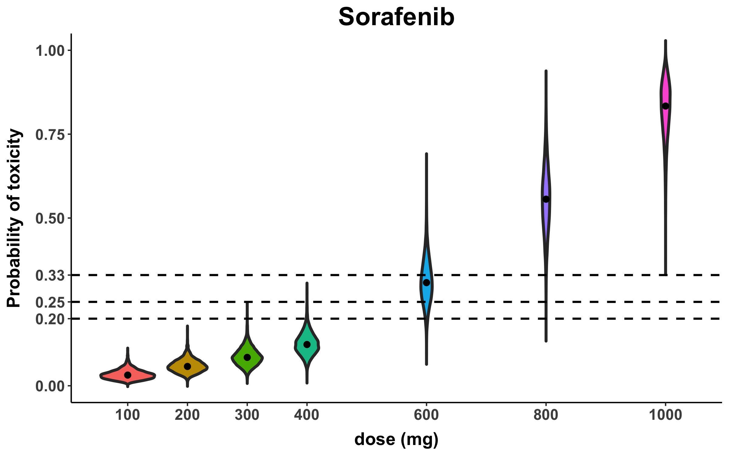
We applied the MADF method, with the same setting and prior distributions as described in the previous section, to both examples introduced in Section 2. Regarding the sorafenib example, Figure 5 shows the posterior distribution obtained for the probability of toxicity associated to each dose panel level. Using the posterior median variant of (11), we obtain the following estimates (0.032, 0.058, 0.085, 0.123, 0.307, 0.556, 0.834). This leads to selecting dose 600 mg as MTD if or , while 400 mg is chosen when . Adopting the EWOC rules as in (12), that is computing , we obtain (0, 0, 0, 0, 0.369, 0.991, 1), (0, 0, 0, 0.002, 0.832, 1, 1) and (0, 0, 0.001, 0.016, 0.964, 1, 1) for , and , respectively. Setting , we select dose 400 mg in all cases.
5.2 The irinotecan / S-1 example
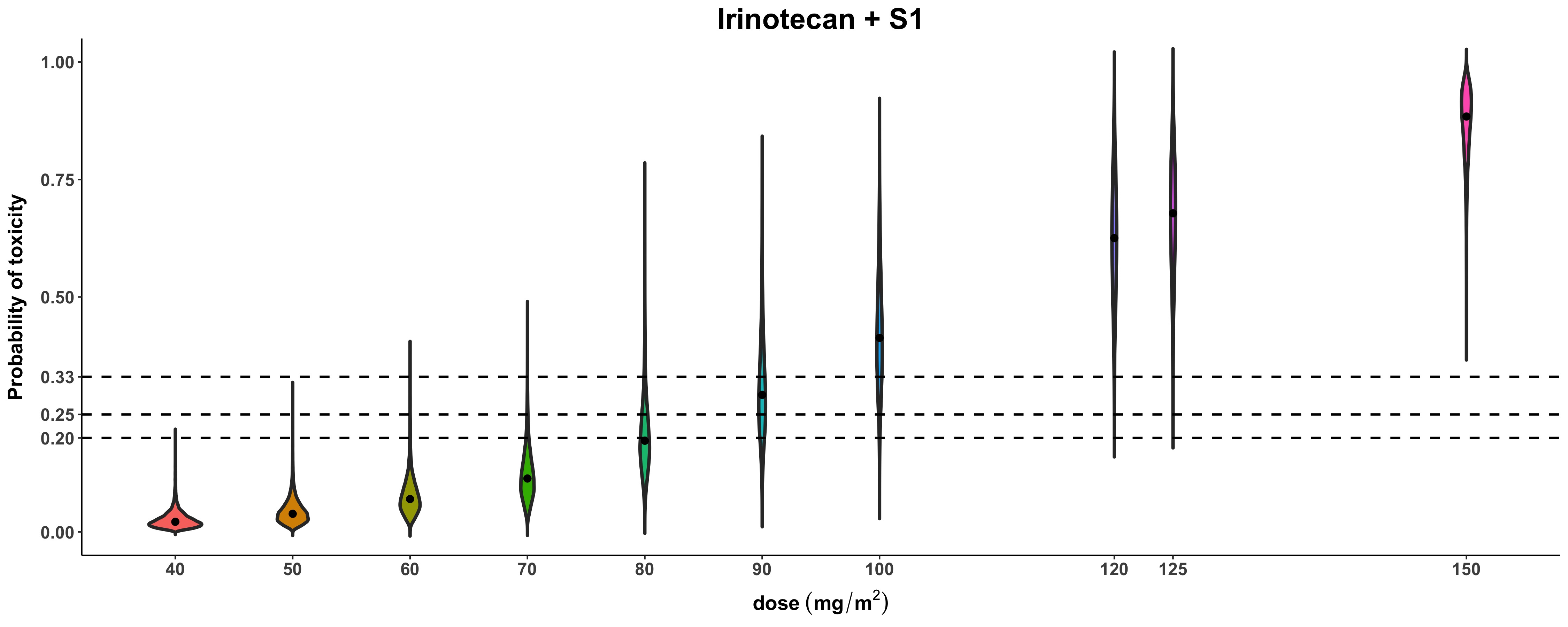
Results of the irinotecan + S-1 example are shown in Figure 6. Differently from before, here , while has the same specification as before. Again, using the posterior median variant of (11), we obtain the following estimates (0.022, 0.039, 0.070, 0.114, 0.194, 0.292, 0.413, 0.625, 0.678, 0.884). This leads to selecting dose 90 mg/m2 as MTD if or , while 80 mg/m2 is chosen when . Adopting the EWOC rules as in (12), we obtain (0, 0, 0, 0.004, 0.061, 0.349, 0.773, 0.990, 0.996, 1), (0, 0, 0.002, 0.027, 0.238, 0.677, 0.944, 0.998, 1, 1) and (0, 0.001, 0.008, 0.082, 0.466, 0.866, 0.984, 1, 1, 1) for , and , respectively. Setting , we select dose 80 mg/m2 in the first two cases and 70 mg/m2 in the last one.
6 Discussion
We proposed a new methodology for random-effects meta-analysis of phase I dose-finding trials, based on a Gaussian process for the random effect structure, and a Gamma process as a prior distribution for the fixed effects. The Gaussian process permits to share more information when doses are closer and less information when they are distant. In this way, for example, regarding a dose panel, dose level 3 and 4 are more correlated than dose level 1 and 4. And the amount of correlation depends on the distance, that seems more logical than assuming a constant value for the correlation. The Gamma prior process preserves the monotonicity assumption of toxicity. We do not suggest to add the full process to be estimated, since, in our experience, even if in meta-analysis more data are available than a single dose-finding trial, data are still not sufficient for a good estimation of the process parameters (results not shown in the paper). To note, we focused on modelling toxicities exactly at the doses that had also been investigated in the analysed trials. In general, in case of rich data and when the estimation of the underlying Gamma process is feasible, the full model actually also allows to interpolate or extrapolate across the continuum of doses. In this case, guidance on how to set the prior distributions can be found in Gelman et al. 2008.
Since the two metrics used in the fixed effect prior and random effect, that is and , respectively, are linked to each others via linear transformation, one can also consider to use the same metric and scaling the prior distributions accordingly.
With the above model specifications, we have generalized the BNHM, as an obvious approach for the single-dose case, to the case of several adjacent doses. Note that for the special case of a single dose, we actually again recover the BNHM with the parameters and corresponding to the overall mean and heterogeneity parameters.
In our results, ZKO had lower PCS performance. This is expected, since this method does not take into account the heterogeneity between trials. Also as expected, PCSs decrease when heterogeneity increases and when only 3+3 dose-finding trials are incorporated in meta-analysis (scenario 5 and 8, respectively). MADF showed to be stable to models misspecification, as we can see in the results of scenario 6 and 7 compared to scenario 2 and 3, respectively. On the other hand, prior specification and simpler models, as MADF3 and MADF4 can give different operating characteristic. A conservative Gamma process prior, as MADF1, has better PCS when the MTD is located at the beginning of the dose panel. Actually, this situation is not very realistic, since it would imply that really few safe doses where repeatedly tested in several clinical trials.
Appendix
Sensitivity analysis tables
Tables 6 and 7 show the full results, in terms of percentage of MTD selection, of the sensitivity analysis performed.
| Dose levels | |||||||
|---|---|---|---|---|---|---|---|
| 1 | 2 | 3 | 4 | 5 | 6 | 7 | |
| Scenario 1 | |||||||
| MADF1 | 0.000 | 0.118 | 0.804 | 0.078 | 0.000 | 0.000 | 0.000 |
| MADF2 | 0.000 | 0.071 | 0.690 | 0.232 | 0.007 | 0.000 | 0.000 |
| MADF3 | 0.000 | 0.049 | 0.508 | 0.422 | 0.021 | 0.000 | 0.000 |
| MADF4 | 0.000 | 0.045 | 0.456 | 0.406 | 0.088 | 0.004 | 0.001 |
| Scenario 2 | |||||||
| MADF1 | 0.000 | 0.000 | 0.079 | 0.908 | 0.013 | 0.000 | 0.000 |
| MADF2 | 0.000 | 0.000 | 0.043 | 0.897 | 0.060 | 0.000 | 0.000 |
| MADF3 | 0.000 | 0.000 | 0.017 | 0.882 | 0.101 | 0.000 | 0.000 |
| MADF4 | 0.000 | 0.000 | 0.026 | 0.840 | 0.131 | 0.003 | 0.000 |
| Scenario 3 | |||||||
| MADF1 | 0.000 | 0.000 | 0.000 | 0.229 | 0.735 | 0.036 | 0.000 |
| MADF2 | 0.000 | 0.000 | 0.000 | 0.101 | 0.709 | 0.185 | 0.005 |
| MADF3 | 0.000 | 0.000 | 0.000 | 0.056 | 0.773 | 0.171 | 0.000 |
| MADF4 | 0.000 | 0.000 | 0.000 | 0.061 | 0.554 | 0.329 | 0.056 |
| Scenario 4 | |||||||
| MADF1 | 0.000 | 0.000 | 0.000 | 0.002 | 0.354 | 0.638 | 0.006 |
| MADF2 | 0.000 | 0.000 | 0.000 | 0.000 | 0.132 | 0.758 | 0.110 |
| MADF3 | 0.000 | 0.000 | 0.000 | 0.000 | 0.139 | 0.819 | 0.042 |
| MADF4 | 0.000 | 0.000 | 0.000 | 0.000 | 0.078 | 0.585 | 0.337 |
| Scenario 5 | |||||||
| MADF1 | 0.000 | 0.001 | 0.216 | 0.747 | 0.036 | 0.000 | 0.000 |
| MADF2 | 0.000 | 0.001 | 0.105 | 0.734 | 0.156 | 0.004 | 0.000 |
| MADF3 | 0.000 | 0.000 | 0.043 | 0.653 | 0.303 | 0.001 | 0.000 |
| MADF4 | 0.000 | 0.000 | 0.051 | 0.575 | 0.337 | 0.037 | 0.000 |
| Scenario 6 | |||||||
| MADF1 | 0.000 | 0.000 | 0.053 | 0.918 | 0.029 | 0.000 | 0.000 |
| MADF2 | 0.000 | 0.000 | 0.028 | 0.892 | 0.080 | 0.000 | 0.000 |
| MADF3 | 0.000 | 0.000 | 0.009 | 0.820 | 0.171 | 0.000 | 0.000 |
| MADF4 | 0.000 | 0.000 | 0.022 | 0.798 | 0.172 | 0.008 | 0.000 |
| Scenario 7 | |||||||
| MADF1 | 0.000 | 0.000 | 0.000 | 0.208 | 0.751 | 0.041 | 0.000 |
| MADF2 | 0.000 | 0.000 | 0.001 | 0.088 | 0.696 | 0.210 | 0.005 |
| MADF3 | 0.000 | 0.000 | 0.000 | 0.049 | 0.753 | 0.198 | 0.000 |
| MADF4 | 0.000 | 0.000 | 0.000 | 0.050 | 0.534 | 0.349 | 0.067 |
| Scenario 8 | |||||||
| MADF1 | 0.000 | 0.000 | 0.003 | 0.338 | 0.630 | 0.029 | 0.000 |
| MADF2 | 0.000 | 0.000 | 0.002 | 0.149 | 0.647 | 0.192 | 0.010 |
| MADF3 | 0.000 | 0.000 | 0.000 | 0.085 | 0.730 | 0.185 | 0.000 |
| MADF4 | 0.000 | 0.000 | 0.001 | 0.077 | 0.511 | 0.339 | 0.072 |
| Scenario 9 | |||||||
| MADF1 | 0.000 | 0.000 | 0.001 | 0.167 | 0.773 | 0.059 | 0.000 |
| MADF2 | 0.000 | 0.000 | 0.000 | 0.091 | 0.699 | 0.205 | 0.005 |
| MADF3 | 0.000 | 0.000 | 0.000 | 0.044 | 0.771 | 0.185 | 0.000 |
| MADF4 | 0.000 | 0.000 | 0.000 | 0.048 | 0.578 | 0.331 | 0.043 |
| Dose levels | |||||||
|---|---|---|---|---|---|---|---|
| 1 | 2 | 3 | 4 | 5 | 6 | 7 | |
| Scenario 1 | |||||||
| MADF1 | 0.004 | 0.213 | 0.637 | 0.138 | 0.008 | 0.000 | 0.000 |
| MADF2 | 0.005 | 0.142 | 0.585 | 0.235 | 0.030 | 0.003 | 0.000 |
| MADF3 | 0.007 | 0.117 | 0.463 | 0.361 | 0.051 | 0.001 | 0.000 |
| MADF4 | 0.003 | 0.112 | 0.457 | 0.317 | 0.093 | 0.017 | 0.001 |
| Scenario 2 | |||||||
| MADF1 | 0.000 | 0.002 | 0.163 | 0.796 | 0.038 | 0.001 | 0.000 |
| MADF2 | 0.000 | 0.002 | 0.095 | 0.817 | 0.084 | 0.002 | 0.000 |
| MADF3 | 0.000 | 0.000 | 0.046 | 0.801 | 0.152 | 0.001 | 0.000 |
| MADF4 | 0.000 | 0.000 | 0.058 | 0.766 | 0.170 | 0.005 | 0.001 |
| Scenario 3 | |||||||
| MADF1 | 0.000 | 0.000 | 0.011 | 0.333 | 0.588 | 0.068 | 0.000 |
| MADF2 | 0.000 | 0.000 | 0.003 | 0.206 | 0.599 | 0.178 | 0.014 |
| MADF3 | 0.000 | 0.000 | 0.001 | 0.132 | 0.659 | 0.205 | 0.003 |
| MADF4 | 0.000 | 0.000 | 0.001 | 0.116 | 0.555 | 0.253 | 0.075 |
| Scenario 4 | |||||||
| MADF1 | 0.000 | 0.000 | 0.001 | 0.034 | 0.456 | 0.488 | 0.021 |
| MADF2 | 0.000 | 0.000 | 0.000 | 0.010 | 0.250 | 0.634 | 0.106 |
| MADF3 | 0.000 | 0.000 | 0.000 | 0.001 | 0.246 | 0.673 | 0.080 |
| MADF4 | 0.000 | 0.000 | 0.000 | 0.002 | 0.151 | 0.568 | 0.279 |
| Scenario 5 | |||||||
| MADF1 | 0.000 | 0.019 | 0.284 | 0.614 | 0.079 | 0.004 | 0.000 |
| MADF2 | 0.000 | 0.015 | 0.187 | 0.589 | 0.191 | 0.016 | 0.002 |
| MADF3 | 0.000 | 0.011 | 0.097 | 0.578 | 0.301 | 0.013 | 0.000 |
| MADF4 | 0.000 | 0.009 | 0.104 | 0.531 | 0.286 | 0.065 | 0.005 |
| Scenario 6 | |||||||
| MADF1 | 0.000 | 0.000 | 0.129 | 0.812 | 0.057 | 0.002 | 0.000 |
| MADF2 | 0.000 | 0.000 | 0.082 | 0.802 | 0.111 | 0.005 | 0.000 |
| MADF3 | 0.000 | 0.000 | 0.045 | 0.769 | 0.179 | 0.007 | 0.000 |
| MADF4 | 0.000 | 0.000 | 0.053 | 0.731 | 0.186 | 0.028 | 0.002 |
| Scenario 7 | |||||||
| MADF1 | 0.000 | 0.000 | 0.013 | 0.317 | 0.600 | 0.070 | 0.000 |
| MADF2 | 0.000 | 0.000 | 0.004 | 0.170 | 0.610 | 0.202 | 0.014 |
| MADF3 | 0.000 | 0.000 | 0.001 | 0.123 | 0.658 | 0.214 | 0.004 |
| MADF4 | 0.000 | 0.000 | 0.002 | 0.104 | 0.516 | 0.290 | 0.088 |
| Scenario 8 | |||||||
| MADF1 | 0.000 | 0.000 | 0.042 | 0.413 | 0.500 | 0.044 | 0.001 |
| MADF2 | 0.000 | 0.000 | 0.015 | 0.232 | 0.554 | 0.181 | 0.018 |
| MADF3 | 0.000 | 0.001 | 0.005 | 0.150 | 0.645 | 0.192 | 0.007 |
| MADF4 | 0.000 | 0.000 | 0.005 | 0.141 | 0.514 | 0.248 | 0.092 |
| Scenario 9 | |||||||
| MADF1 | 0.000 | 0.000 | 0.008 | 0.271 | 0.635 | 0.085 | 0.001 |
| MADF2 | 0.000 | 0.000 | 0.005 | 0.173 | 0.622 | 0.189 | 0.011 |
| MADF3 | 0.000 | 0.000 | 0.002 | 0.114 | 0.684 | 0.196 | 0.004 |
| MADF4 | 0.000 | 0.000 | 0.005 | 0.095 | 0.552 | 0.279 | 0.069 |
References
- Awada et al. (2005) A. Awada, A. Hendlisz, T. Gil, S. Bartholomeus, M. Mano, D. De Valeriola, D. Strumberg, E. Brendel, C. G. Haase, B. Schwartz, et al. Phase I safety and pharmacokinetics of BAY 43-9006 administered for 21 days on / 7 days off in patients with advanced, refractory solid tumours. British Journal of Cancer, 92(10):1855, 2005.
- Babb et al. (1998) J. Babb, A. Rogatko, and S. Zacks. Cancer phase I clinical trials: efficient dose escalation with overdose control. Statistics in Medicine, 17(10):1103–1120, 1998.
- Borthakur et al. (2011) G. Borthakur, H. Kantarjian, F. Ravandi, W. Zhang, M. Konopleva, J. J. Wright, S. Faderl, S. Verstovsek, S. Mathews, M. Andreeff, et al. Phase I study of sorafenib in patients with refractory or relapsed acute leukemias. Haematologica, 96(1):62–68, 2011.
- Bretz et al. (2005) F. Bretz, J. C. Pinheiro, and M. Branson. Combining multiple comparisons and modeling techniques in dose-response studies. Biometrics, 61(3):738–748, 2005.
- Chen et al. (2014) Y.-B. Chen, S. Li, A. A. Lane, C. Connolly, C. Del Rio, B. Valles, M. Curtis, K. Ballen, C. Cutler, B. R. Dey, et al. Phase I trial of maintenance sorafenib after allogeneic hematopoietic stem cell transplantation for fms-like tyrosine kinase 3 internal tandem duplication acute myeloid leukemia. Biology of Blood and Marrow Transplantation, 20(12):2042–2048, 2014.
- Cheung (2011) Y. K. Cheung. Dose finding by the continual reassessment method. Chapman and Hall/CRC, 2011.
- Chevret (2006) S. Chevret. Statistical methods for dose-finding experiments of Statistics in practice. John Wiley and Sons, Chichester, West Sussex, England, 2006.
- Clark et al. (2005) J. W. Clark, J. P. Eder, D. Ryan, C. Lathia, and H.-J. Lenz. Safety and pharmacokinetics of the dual action Raf kinase and vascular endothelial growth factor receptor inhibitor, BAY 43-9006, in patients with advanced, refractory solid tumors. Clinical Cancer Research, 11(15):5472–5480, 2005.
- Crump et al. (2010) M. Crump, D. Hedley, S. Kamel-Reid, B. Leber, R. Wells, J. Brandwein, R. Buckstein, J. Kassis, M. Minden, J. Matthews, et al. A randomized phase I clinical and biologic study of two schedules of sorafenib in patients with myelodysplastic syndrome or acute myeloid leukemia: a NCIC (National Cancer Institute of Canada) clinical trials group study. Leukemia & Lymphoma, 51(2):252–260, 2010.
- Doob (1942) J. L. Doob. The Brownian movement and stochastic equations. Annals of Mathematics, 42:351–369, 1942.
- Friede et al. (2017) T. Friede, C. Röver, S. Wandel, and B. Neuenschwander. Meta-analysis of few small studies in orphan diseases. Research Synthesis Methods, 8(1):79–91, 2017.
- Furuse et al. (2008) J. Furuse, H. Ishii, K. Nakachi, E. Suzuki, S. Shimizu, and K. Nakajima. Phase I study of sorafenib in Japanese patients with hepatocellular carcinoma. Cancer Science, 99(1):159–165, 2008.
- Gelman et al. (2008) A. Gelman, A. Jakulin, M. G. Pittau, and Y.-S. Su. A weakly informative default prior distribution for logistic and other regression models. The Annals of Applied Statistics, 2(4):1360–1383, Dec. 2008. doi: 10.1214/08-AOAS191.
- Gelman et al. (2014) A. Gelman, J. B. Carlin, H. Stern, D. B. Dunson, A. Vehtari, and D. B. Rubin. Bayesian data analysis. Chapman & Hall / CRC, Boca Raton, 3rd edition, 2014.
- Goya et al. (2012) H. Goya, H. Kuraishi, S. Koyama, T. Ichiyama, F. Yoshiike, K. Hirai, T. Agatsuma, K. Tateishi, S. Kanda, H. Yamamoto, et al. Phase I/II study of S-1 combined with biweekly irinotecan chemotherapy in previously treated advanced non-small cell lung cancer. Cancer Chemotherapy and Pharmacology, 70(5):691–697, 2012.
- Günhan et al. (2019) B. K. Günhan, S. Röver, and T. Friede. Meta-analysis of few studies involving rare events. Research Synthesis Methods, in press, 2019. doi: 10.1002/jrsm.1370.
- Inokuchi et al. (2006) M. Inokuchi, T. Yamashita, H. Yamada, K. Kojima, W. Ichikawa, Z. Nihei, T. Kawano, and K. Sugihara. Phase I/II study of S-1 combined with irinotecan for metastatic advanced gastric cancer. British Journal of Cancer, 94(8):1130, 2006.
- Ishimoto et al. (2009) O. Ishimoto, T. Ishida, Y. Honda, M. Munakata, and S. Sugawara. Phase I study of daily S-1 combined with weekly irinotecan in patients with advanced non-small cell lung cancer. International Journal of Clinical Oncology, 14(1):43–47, 2009.
- Jackson et al. (2018) D. Jackson, M. Law, T. Stijnen, W. Viechtbauer, and I. R. White. A comparison of seven random-effects models for meta-analyses that estimate the summary odds ratio. Statistics in Medicine, 37(7):1059–1085, Mar. 2018. doi: 10.1002/sim.7588.
- Jia et al. (2013) N. Jia, I. Liou, J. Halldorson, R. Carithers, J. Perkins, J. Reyes, M. Yeh, E. Stohr, S. Rao, and E. H. Lin. Phase I adjuvant trial of sorafenib in patients with hepatocellular carcinoma after orthotopic liver transplantation. Anticancer Research, 33(6):2797–2800, 2013.
- Komatsu et al. (2010) Y. Komatsu, S. Yuki, N. Fuse, T. Kato, T. Miyagishima, M. Kudo, Y. Kunieda, M. Tateyama, O. Wakahama, T. Meguro, et al. Phase 1/2 clinical study of irinotecan and oral S-1 (IRIS) in patients with advanced gastric cancer. Advances in Therapy, 27(7):483–492, 2010.
- Kusaba et al. (2010) H. Kusaba, T. Esaki, K. Futami, S. Tanaka, H. Fujishima, K. Mitsugi, K. Sakai, H. Ariyama, R. Tanaka, N. Kinugawa, et al. Phase I/II study of a 3-week cycle of irinotecan and S-1 in patients with advanced colorectal cancer. Cancer Science, 101(12):2591–2595, 2010.
- Lawless and Crowder (2004) J. Lawless and M. Crowder. Covariates and random effects in a gamma process model with application to degradation and failure. Lifetime Data Analysis, 10(3):213–227, 2004.
- Le Tourneau et al. (2009) C. Le Tourneau, J. J. Lee, and L. L. Siu. Dose escalation methods in phase I cancer clinical trials. Journal of the National Cancer Institute, 101(10):708–720, 2009.
- Miller et al. (2009) A. A. Miller, D. J. Murry, K. Owzar, D. R. Hollis, E. B. Kennedy, G. Abou-Alfa, A. Desai, J. Hwang, M. A. Villalona-Calero, E. C. Dees, et al. Phase I and pharmacokinetic study of sorafenib in patients with hepatic or renal dysfunction: CALGB 60301. Journal of Clinical Oncology, 27(11):1800, 2009.
- Minami et al. (2008) H. Minami, K. Kawada, H. Ebi, K. Kitagawa, Y.-i. Kim, K. Araki, H. Mukai, M. Tahara, H. Nakajima, and K. Nakajima. Phase I and pharmacokinetic study of sorafenib, an oral multikinase inhibitor, in Japanese patients with advanced refractory solid tumors. Cancer Science, 99(7):1492–1498, 2008.
- Moore et al. (2005) M. Moore, H. Hirte, L. Siu, A. Oza, S. Hotte, O. Petrenciuc, F. Cihon, C. Lathia, and B. Schwartz. Phase I study to determine the safety and pharmacokinetics of the novel Raf kinase and VEGFR inhibitor BAY 43-9006, administered for 28 days on / 7 days off in patients with advanced, refractory solid tumors. Annals of Oncology, 16(10):1688–1694, 2005.
- Morita et al. (2008) S. Morita, P. Thall, and P. Müller. Determining the effective sample size of a parametric prior. Biometrics, 64(2):595–602, June 2008. doi: 10.1111/j.1541-0420.2007.00888.x.
- Nabors et al. (2011) L. Nabors, J. Supko, M. Rosenfeld, M. Chamberlain, S. Phuphanich, T. Batchelor, S. Desideri, X. Ye, J. Wright, S. Gujar, et al. Phase I trial of sorafenib in patients with recurrent or progressive malignant glioma. Neuro-Oncology, 13(12):1324–1330, 2011.
- Nakafusa et al. (2008) Y. Nakafusa, M. Tanaka, T. Ohtsuka, A. Miyoshi, N. Kohya, Y. Kitajima, S. Sato, S. Mochinaga, S. Dohi, and K. Miyazaki. Phase I/II study of combination therapy with s-1 and cpt-11 for metastatic colorectal cancer. Molecular Medicine Reports, 1(6):925–930, 2008.
- Neuenschwander et al. (2008) B. Neuenschwander, M. Branson, and T. Gsponer. Critical aspects of the Bayesian approach to phase I cancer trials. Statistics in Medicine, 27(13):2420–2439, June 2008. doi: 10.1002/sim.3230.
- Neuenschwander et al. (2015) B. Neuenschwander, A. Matano, Z. Tang, S. Roychoudhury, S. Wandel, and S. Bailey. A Bayesian industry approach to phase I combination trials in oncology. In W. Zhao and H. Yang, editors, Statistical methods in drug combination studies, chapter 6, pages 95–135. Chapman & Hall / CRC, Boca Raton, 2015.
- Ogata et al. (2009) Y. Ogata, T. Sasatomi, Y. Akagi, N. Ishibashi, S. Mori, and K. Shirouzu. Dosage escalation study of S-1 and irinotecan in metronomic chemotherapy against advanced colorectal cancer. The Kurume Medical Journal, 56(1+ 2):1–7, 2009.
- O’Quigley and Zohar (2010) J. O’Quigley and S. Zohar. Retrospective robustness of the continual reassessment method. J Biopharm Stat, 20(5):1013–1025, Sep 2010.
- O’Quigley et al. (1990) J. O’Quigley, M. Pepe, and L. Fisher. Continual reassessment method: a practical design for phase 1 clinical trials in cancer. Biometrics, pages 33–48, 1990.
- Schwinghammer and Kroboth (1988) T. L. Schwinghammer and P. D. Kroboth. Basic concepts in pharmacodynamic modeling. Journal of Clinical Pharmacology, 28(5):388–394, May 1988. doi: 10.1002/j.1552-4604.1988.tb05745.x.
- Shiozawa et al. (2009) M. Shiozawa, N. Sugano, K. Tsuchida, S. Morinaga, M. Akaike, and Y. Sugimasa. A phase I study of combination therapy with S-1 and irinotecan (CPT-11) in patients with advanced colorectal cancer. Journal of Cancer Research and Clinical Oncology, 135(3):365–370, 2009.
- Steutel (1979) F. W. Steutel. Infinite divisibilty in theory and practice. Scandinavian Journal of Statistics, 6(2):57–64, 1979.
- Strumberg et al. (2005) D. Strumberg, H. Richly, R. A. Hilger, N. Schleucher, S. Korfee, M. Tewes, M. Faghih, E. Brendel, D. Voliotis, C. G. Haase, et al. Phase I clinical and pharmacokinetic study of the novel Raf kinase and vascular endothelial growth factor receptor inhibitor BAY 43-9006 in patients with advanced refractory solid tumors. Journal of Clinical Oncology, 23(5):965–972, 2005.
- Takiuchi et al. (2005) H. Takiuchi, H. Narahara, T. Tsujinaka, M. Gotoh, S.-i. Kawabe, K.-i. Katsu, H. Iishi, M. Tatsuta, K. Fujitani, H. Furukawa, et al. Phase I study of S-1 combined with irinotecan (CPT-11) in patients with advanced gastric cancer (OGSG 0002). Japanese Journal of Clinical Oncology, 35(9):520–525, 2005.
- Thomas et al. (2014) N. Thomas, K. Sweeney, and V. Somayaji. Meta-analysis of clinical dose-response in a large drug development portfolio. Statistics in Biopharmaceutical Research, 6(4):302–317, 2014.
- Turner et al. (2012) R. M. Turner, J. Davey, M. J. Clarke, S. G. Thompson, and J. P. T. Higgins. Predicting the extent of heterogeneity in meta-analysis, using empirical data from the Cochrane Database of Systematic Reviews. International Journal of Epidemiology, 41(3):818–827, June 2012. doi: 10.1093/ije/dys041.
- Uhlenbeck and Ornstein (1930) G. E. Uhlenbeck and L. S. Ornstein. On the theory of Brownian motion. Physical Review, 36(5):823–841, Sept. 1930. doi: 10.1103/PhysRev.36.823.
- Ursino et al. (2019) M. Ursino, Y. Yuan, C. Alberti, E. Comets, G. Favrais, T. Friede, F. Lentz, N. Stallard, and S. Zohar. A dose finding design for seizure reduction in neonates. Journal of the Royal Statistical Society: Series C (Applied Statistics), 68(2):427–444, 2019.
- Yoda et al. (2011) S. Yoda, K. Soejima, H. Yasuda, K. Naoki, I. Kawada, H. Watanabe, I. Nakachi, R. Satomi, S. Nakayama, S. Ikemura, et al. A phase I study of S-1 and irinotecan combination therapy in previously treated advanced non-small cell lung cancer patients. Cancer Chemotherapy and Pharmacology, 67(3):717–722, 2011.
- Zohar et al. (2011) S. Zohar, S. Katsahian, and J. O’Quigley. An approach to meta-analysis of dose-finding studies. Statistics in Medicine, 30(17):2109–2116, 2011. doi: 10.1002/sim.4121.